Cited by 83

The DOI matches its Crossref record; 14 of the 14 references it cites were found in a registry or an index.

Quantifying the stochastic component of epigenetic aging

Tong, Huige, Dwaraka, Varun B., Chen, Qingwen, Luo, Qi, Lasky-Su, Jessica A., Smith, Ryan, Teschendorff, Andrew E.·2024·Nature Aging

Abstract

DNA methylation clocks can accurately estimate chronological age and, to some extent, also biological age, yet the process by which age-associated DNA methylation (DNAm) changes are acquired appears to be quasi-stochastic, raising a fundamental question: how much of an epigenetic clock’s predictive accuracy could be explained by a stochastic process of DNAm change? Here, using DNAm data from sorted immune cells, we build realistic simulation models, subsequently demonstrating in over 22,770 sorted and whole-blood samples from 25 independent cohorts that approximately 66–75% of the accuracy underpinning Horvath’s clock could be driven by a stochastic process. This fraction increases to 90% for the more accurate Zhang’s clock, but is lower (63%) for the PhenoAge clock, suggesting that biological aging is reflected by nonstochastic processes. Confirming this, we demonstrate that Horvath’s age acceleration in males and PhenoAge’s age acceleration in severe coronavirus disease 2019 cases and smokers are not driven by an increased rate of stochastic change but by nonstochastic processes. These results significantly deepen our understanding and interpretation of epigenetic clocks.

Overview

The claims and statistics of this paper haven’t been checked yet.

Run the check — free, no account needed. It reads the open-access text and checks the sources it cites.

A few free checks a day · papers already verified open instantly · results are public

Integrity signals

Registry

Crossref · 10.1038/s43587-024-00600-8

Cites

14 of 14 references verified0 citation errors · 0 not checkable

Statistics

Figures

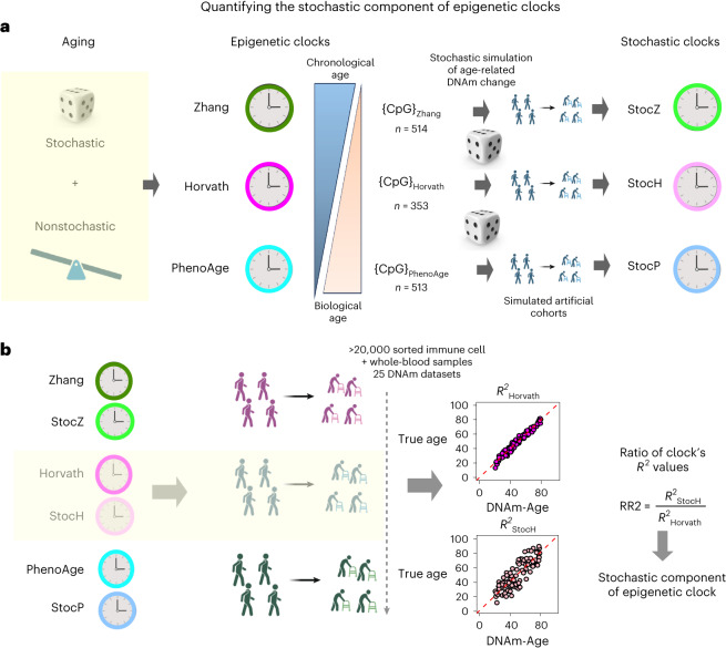
Fig. 1 The overall strategy to quantify the stochastic component of epigenetic clocks. a, The original epigenetic clocks are constructed from real DNAm data describing a real aging process that includes both stochastic and nonstochastic elements. The key idea is to simulate a realistic stochastic process of DNAm change accrual at the same CpG sites that make up the original clocks. In effect, this ‘replaces’ the real aging process with a pure stochastic one at the same sites. With the simulation model in place, one can then generate artificial cohorts from which machine learning predictor of age can be derived, defining the ‘stochastic clock’ analogs. b, We then apply the original and stochastic clocks to a large collection of DNAm datasets representing both sorted immune cells (to gauge the effect of CTH) and whole-blood tissue. The ratio of R2 values between the stochastic clock and its original counterpart provides a direct quantification of the stochastic component of that clock. Created with Biorender.com.
Fig. 1 The overall strategy to quantify the stochastic component of epigenetic clocks. a, The original epigenetic clocks are constructed from real DNAm data describing a real aging process that includes both stochastic and nonstochastic elements. The key idea is to simulate a realistic stochastic process of DNAm change accrual at the same CpG sites that make up the original clocks. In effect, this ‘replaces’ the real aging process with a pure stochastic one at the same sites. With the simulation model in place, one can then generate artificial cohorts from which machine learning predictor of age can be derived, defining the ‘stochastic clock’ analogs. b, We then apply the original and stochastic clocks to a large collection of DNAm datasets representing both sorted immune cells (to gauge the effect of CTH) and whole-blood tissue. The ratio of R2 values between the stochastic clock and its original counterpart provides a direct quantification of the stochastic component of that clock. Created with Biorender.com.CC BY · PubMed Central
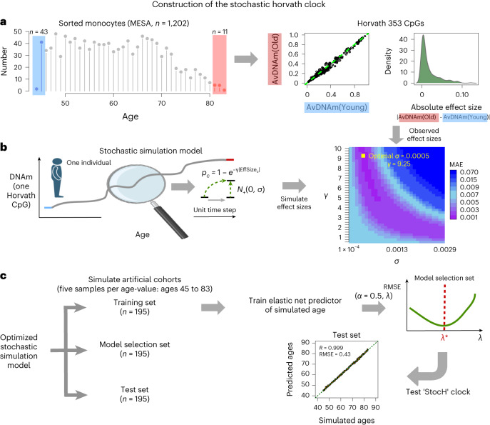
Fig. 2 Construction of the StocH clock. a, Left: the age distribution of the 1,202 sorted monocyte samples from the MESA study. The shaded blue and red regions highlight the youngest and oldest samples used in the simulation, respectively. Middle: the average DNAm over the youngest (AvDNAm(Young)) and oldest (AvDNAm(Old)) samples for each of the 353 Horvath Clock CpGs. Right: the corresponding density of absolute effect sizes defined as the magnitude of the DNAm difference between youngest and oldest samples. b, The stochastic simulation of one CpG in one individual of a given age, which starts out from the average DNAm in the youngest samples and subsequently adds a stochastic deviate for each unit time step. The probability per time step that a CpG is altered is given by a decaying exponential with exponent determined by the observed absolute effect size of the CpG and a CpG-independent parameter, γ, that controls the overall probability of CpGs changing. The direction of the DNAm change is dictated by the directionality of the observed effect size, with the magnitude determined by the standard deviation, σ, of a signed Gaussian distribution, as indicated. Of note, the simulation model adds Gaussian deviates to the quantiles of an inverse normal distribution. The model is simulated to generate effect sizes for each of the 353 CpGs, which is then compared with the observed distribution to identify the optimal (λ and σ) parameters minimizing the MAE between simulated and observed values. c, To build the StocH clock, we then use the simulation model with the optimal (λ and σ) parameter values to generate three artificial cohorts of 195 samples each. There are 195 samples because we simulate five samples per age value, with ages ranging between 45 and 83 years; that is, a total of 39 distinct age values. One cohort is used to train elastic net regression models with α=0.5, and for varying penalty parameter values, λ. These models are then evaluated in the model selection set to select the model that optimizes the root mean square error (RMSE). This optimal model is then evaluated in the test set. Created with Biorender.com.
Fig. 2 Construction of the StocH clock. a, Left: the age distribution of the 1,202 sorted monocyte samples from the MESA study. The shaded blue and red regions highlight the youngest and oldest samples used in the simulation, respectively. Middle: the average DNAm over the youngest (AvDNAm(Young)) and oldest (AvDNAm(Old)) samples for each of the 353 Horvath Clock CpGs. Right: the corresponding density of absolute effect sizes defined as the magnitude of the DNAm difference between youngest and oldest samples. b, The stochastic simulation of one CpG in one individual of a given age, which starts out from the average DNAm in the youngest samples and subsequently adds a stochastic deviate for each unit time step. The probability per time step that a CpG is altered is given by a decaying exponential with exponent determined by the observed absolute effect size of the CpG and a CpG-independent parameter, γ, that controls the overall probability of CpGs changing. The direction of the DNAm change is dictated by the directionality of the observed effect size, with the magnitude determined by the standard deviation, σ, of a signed Gaussian distribution, as indicated. Of note, the simulation model adds Gaussian deviates to the quantiles of an inverse normal distribution. The model is simulated to generate effect sizes for each of the 353 CpGs, which is then compared with the observed distribution to identify the optimal (λ and σ) parameters minimizing the MAE between simulated and observed values. c, To build the StocH clock, we then use the simulation model with the optimal (λ and σ) parameter values to generate three artificial cohorts of 195 samples each. There are 195 samples because we simulate five samples per age value, with ages ranging between 45 and 83 years; that is, a total of 39 distinct age values. One cohort is used to train elastic net regression models with α=0.5, and for varying penalty parameter values, λ. These models are then evaluated in the model selection set to select the model that optimizes the root mean square error (RMSE). This optimal model is then evaluated in the test set. Created with Biorender.com.CC BY · PubMed Central
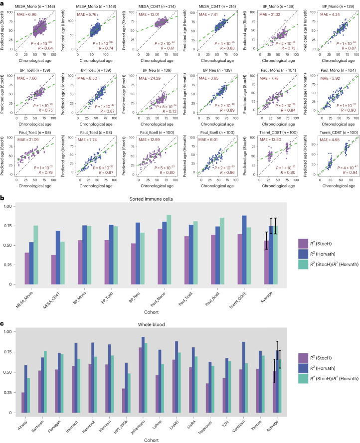
Fig. 3 Quantification of stochastic component of Horvath’s clock. a, Scatter plots of predicted age versus chronological (true) age for the StocH clock (purple) and Horvath’s clock (slate blue) in various sorted immune cell datasets as indicated. The number of sorted samples in dataset is indicated at the top alongside the name of the cohort/study. In addition, we provide the MAE, R-value and corresponding nominal correlation-test two-tailed P value in each plot. b, A bar plot comparing R2 values of the StocH clock and Horvath’s clock in each of the datasets. In addition, we also depict the ratio of the R2 value from StocH to the R2 value from Horvath’s clock. The sample sizes of sorted immune cell datasets are as follows: MESA_Mono (n = 1,148), MESA_CD4T (n = 214), BP_Mono (n = 139), BP_Tcell (n = 139), BP_Neu (n = 139), Paul_Mono (n = 104), Paul_Tcell (n = 98), Paul_Bcell (n = 100) and Tserel_CD8T (n = 100). The last set of bars displays the average and standard deviation over all sorted immune cell datasets. c, As in b, but for StocH and Horvath’s clock on 15 whole-blood cohorts. The sample sizes of whole-blood datasets are as follows: Airway (n = 1,032), Barturen (n = 574), Flanagan (n = 184), Hannon1 (n = 636), Hannon2 (n = 665), Hannum (n = 656), HPT_450k (n = 418), Johansson (n = 729), Lehne (n = 2,707), LiuMS (n = 279), LiuRA (n = 689), Tsaprouni (n = 464), TZH (n = 705), Ventham (n = 380) and Zannas (n = 422).
Fig. 3 Quantification of stochastic component of Horvath’s clock. a, Scatter plots of predicted age versus chronological (true) age for the StocH clock (purple) and Horvath’s clock (slate blue) in various sorted immune cell datasets as indicated. The number of sorted samples in dataset is indicated at the top alongside the name of the cohort/study. In addition, we provide the MAE, R-value and corresponding nominal correlation-test two-tailed P value in each plot. b, A bar plot comparing R2 values of the StocH clock and Horvath’s clock in each of the datasets. In addition, we also depict the ratio of the R2 value from StocH to the R2 value from Horvath’s clock. The sample sizes of sorted immune cell datasets are as follows: MESA_Mono (n = 1,148), MESA_CD4T (n = 214), BP_Mono (n = 139), BP_Tcell (n = 139), BP_Neu (n = 139), Paul_Mono (n = 104), Paul_Tcell (n = 98), Paul_Bcell (n = 100) and Tserel_CD8T (n = 100). The last set of bars displays the average and standard deviation over all sorted immune cell datasets. c, As in b, but for StocH and Horvath’s clock on 15 whole-blood cohorts. The sample sizes of whole-blood datasets are as follows: Airway (n = 1,032), Barturen (n = 574), Flanagan (n = 184), Hannon1 (n = 636), Hannon2 (n = 665), Hannum (n = 656), HPT_450k (n = 418), Johansson (n = 729), Lehne (n = 2,707), LiuMS (n = 279), LiuRA (n = 689), Tsaprouni (n = 464), TZH (n = 705), Ventham (n = 380) and Zannas (n = 422).CC BY · PubMed Central
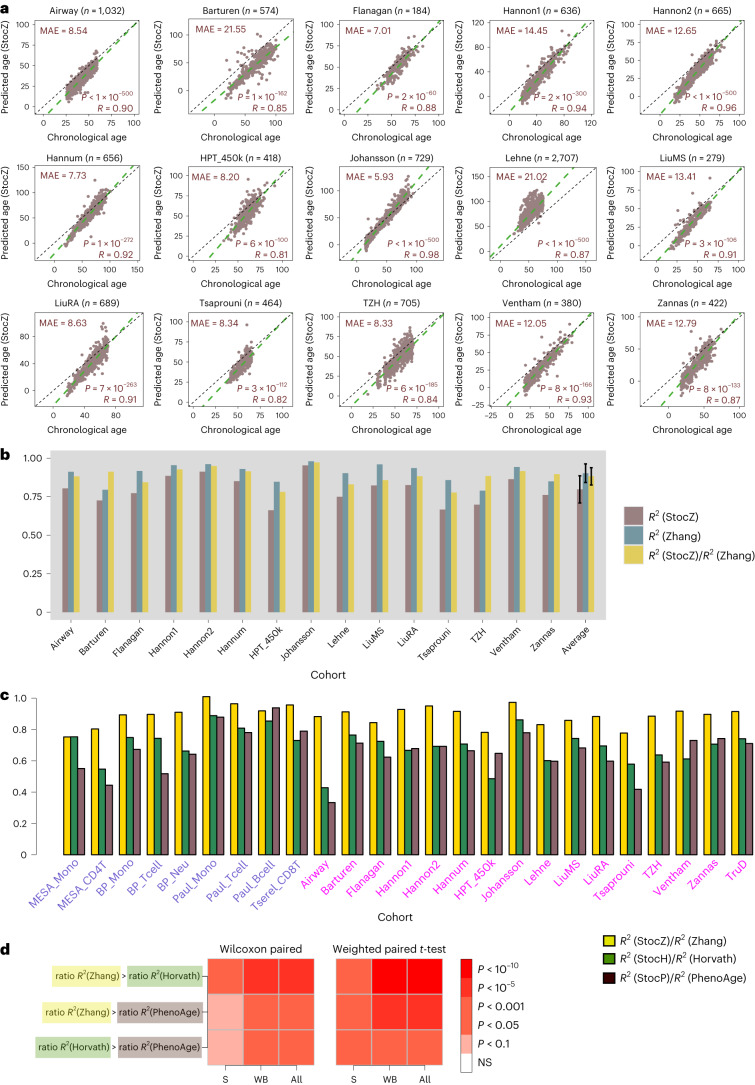
Fig. 4 Stochastic component increases with accuracy of clock. a, Scatter plots of predicted age versus chronological (true) age for the stochastic Zhang clock (StocZ clock) in each of 15 whole-blood datasets. The number of samples in the dataset is indicated at the top alongside the name of the cohort. In addition we provide the MAE, R-value and corresponding nominal correlation-test two-tailed P value in each plot. b, A bar plot comparing R2 values of the StocZ clock and Zhang’s clock in each of the 15 whole-blood datasets. In addition, we also depict the ratio of the R2 value from StocZ to the R2 value from Zhang’s clock. The last set of bars displays the average and standard deviation over the 15 datasets. The sample size of each cohort is given in a. c, A comparison of the ratio of R2 values among Zhang, Horvath and PhenoAge clocks across all sorted and whole-blood datasets. The sample size of the sorted datasets are given in Fig. 3 legend. d, Heat maps displaying meta-analysis P values comparing the ratio of R2 values across the sorted datasets (S), the whole-blood datasets (WB) and all together (All). We provide two sets of P values, one derived from a one-tailed paired Wilcoxon rank sum test over cohorts and another derived by running a weighted linear regression model of the ratios against clock with the cohort as a covariate and using the sample sizes of the cohorts as weights. In the latter case, the P value is two tailed.
Fig. 4 Stochastic component increases with accuracy of clock. a, Scatter plots of predicted age versus chronological (true) age for the stochastic Zhang clock (StocZ clock) in each of 15 whole-blood datasets. The number of samples in the dataset is indicated at the top alongside the name of the cohort. In addition we provide the MAE, R-value and corresponding nominal correlation-test two-tailed P value in each plot. b, A bar plot comparing R2 values of the StocZ clock and Zhang’s clock in each of the 15 whole-blood datasets. In addition, we also depict the ratio of the R2 value from StocZ to the R2 value from Zhang’s clock. The last set of bars displays the average and standard deviation over the 15 datasets. The sample size of each cohort is given in a. c, A comparison of the ratio of R2 values among Zhang, Horvath and PhenoAge clocks across all sorted and whole-blood datasets. The sample size of the sorted datasets are given in Fig. 3 legend. d, Heat maps displaying meta-analysis P values comparing the ratio of R2 values across the sorted datasets (S), the whole-blood datasets (WB) and all together (All). We provide two sets of P values, one derived from a one-tailed paired Wilcoxon rank sum test over cohorts and another derived by running a weighted linear regression model of the ratios against clock with the cohort as a covariate and using the sample sizes of the cohorts as weights. In the latter case, the P value is two tailed.CC BY · PubMed Central
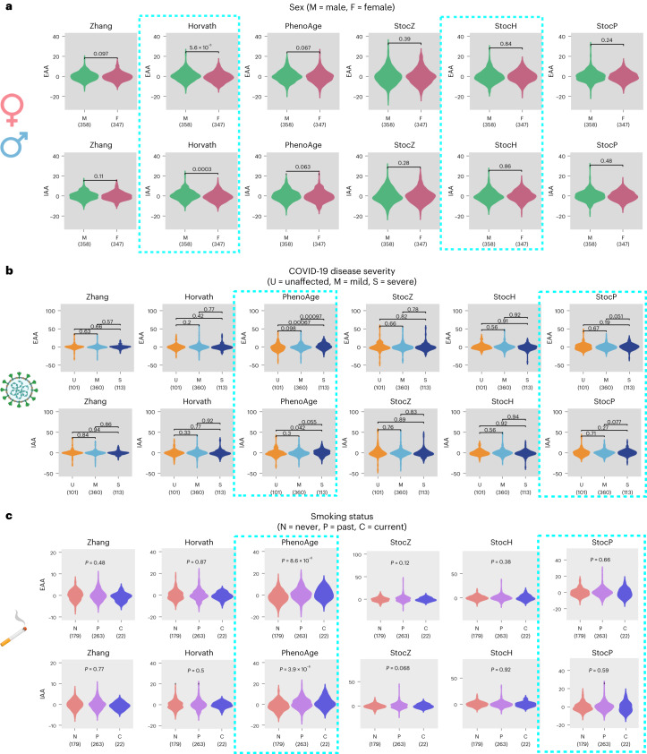
Fig. 5 Age acceleration in males, severe COVID-19 cases and smokers is the result of nonstochastic processes. a, Violin plots for EAA and IAA (adjusted for 12 immune cell type fractions) for Zhang, Horvath and PhenoAge clocks, as well as their stochastic analogs. The P values derive from two-tailed Wilcoxon rank sum tests correlating the age acceleration measures to sex (male (M) and female (F)). Data are displayed for the TZH cohort but results are similar for all other cohorts. The number of samples in each violin plot is given below the violin. b, As in a, but evaluated in the DNAm dataset of Barturen et al., with EAA/IAA being correlated to COVID-19 disease severity, as indicated. c, As in a, but evaluated in the DNAm dataset of Tsaprouni et al., with EAA/IAA being correlated to smoking status. The P values derive from a linear regression test, with smoking status an ordinal variable (never smoker 0, ex-smoker 1 and smoker 2). Created with Biorender.com.
Fig. 5 Age acceleration in males, severe COVID-19 cases and smokers is the result of nonstochastic processes. a, Violin plots for EAA and IAA (adjusted for 12 immune cell type fractions) for Zhang, Horvath and PhenoAge clocks, as well as their stochastic analogs. The P values derive from two-tailed Wilcoxon rank sum tests correlating the age acceleration measures to sex (male (M) and female (F)). Data are displayed for the TZH cohort but results are similar for all other cohorts. The number of samples in each violin plot is given below the violin. b, As in a, but evaluated in the DNAm dataset of Barturen et al., with EAA/IAA being correlated to COVID-19 disease severity, as indicated. c, As in a, but evaluated in the DNAm dataset of Tsaprouni et al., with EAA/IAA being correlated to smoking status. The P values derive from a linear regression test, with smoking status an ordinal variable (never smoker 0, ex-smoker 1 and smoker 2). Created with Biorender.com.CC BY · PubMed Central
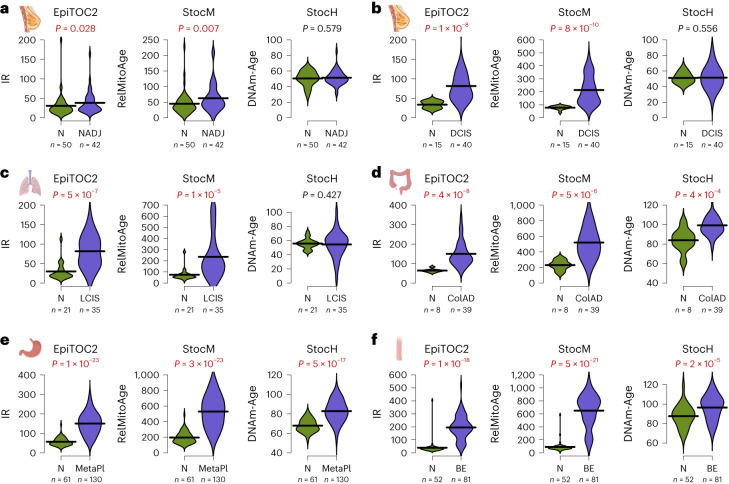
Fig. 6 An increased rate of stochastic change describes mitotic age acceleration in precancer. a, Left: violin plots comparing the IR per year between normal breast from healthy women (N) and normal breast adjacent to breast cancer (NADJ), as estimated using the epigenetic mitotic clock EpiTOC2. The P values are from a one-tailed Wilcoxon test. The number of samples is given below violin. Middle and right: as left, but for the stochastic analog of EpiTOC2 and StocH. Samples between groups are age matched. b, As in a but for a DNAm dataset profiling normal breast tissue and breast DCIS. c, As in a but for a DNAm dataset profiling normal lung tissue and LCIS. d, As in a but for a DNAm dataset profiling normal colon tissue and colon adenoma (ColAD). e, As in a but for a DNAm dataset profiling normal gastric mucosa and gastric metaplasia (MetaPl). f, As in a but for a DNAm dataset profiling normal squamous esophagus and Barrett’s esophagus (BE). Created with Biorender.com.
Fig. 6 An increased rate of stochastic change describes mitotic age acceleration in precancer. a, Left: violin plots comparing the IR per year between normal breast from healthy women (N) and normal breast adjacent to breast cancer (NADJ), as estimated using the epigenetic mitotic clock EpiTOC2. The P values are from a one-tailed Wilcoxon test. The number of samples is given below violin. Middle and right: as left, but for the stochastic analog of EpiTOC2 and StocH. Samples between groups are age matched. b, As in a but for a DNAm dataset profiling normal breast tissue and breast DCIS. c, As in a but for a DNAm dataset profiling normal lung tissue and LCIS. d, As in a but for a DNAm dataset profiling normal colon tissue and colon adenoma (ColAD). e, As in a but for a DNAm dataset profiling normal gastric mucosa and gastric metaplasia (MetaPl). f, As in a but for a DNAm dataset profiling normal squamous esophagus and Barrett’s esophagus (BE). Created with Biorender.com.CC BY · PubMed Central
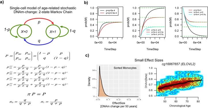
Extended Data Fig. 1 Single-cell stochastic model of DNAm change with age. a) Depiction of a 2-state Markov Chain model with X = 0 representing the unmethylated state of one CpG, X = 1 representing it’s methylated state. P is the stochastic matrix so that row-entries add to 1. π represents the invariant steady-state probability distribution of finding a CpG in one cell unmethylated or methylated. The solution to the dynamics specified by the Markov-Chain as well as the steady-state values are given. b) Examples of how the probability of finding a CpG methylated in one cell changes with timestep for different scenarios specified by p (the probability of methylation), q (the probability of demethylation) and initial conditions. c) Empirically estimated effect sizes for real age-associated CpGs, as derived from a large 450k DNAm dataset of 1202 monocytes. Right scatterplot depicts the top-ranked CpG displaying the largest effect size.
Extended Data Fig. 1 Single-cell stochastic model of DNAm change with age. a) Depiction of a 2-state Markov Chain model with X = 0 representing the unmethylated state of one CpG, X = 1 representing it’s methylated state. P is the stochastic matrix so that row-entries add to 1. π represents the invariant steady-state probability distribution of finding a CpG in one cell unmethylated or methylated. The solution to the dynamics specified by the Markov-Chain as well as the steady-state values are given. b) Examples of how the probability of finding a CpG methylated in one cell changes with timestep for different scenarios specified by p (the probability of methylation), q (the probability of demethylation) and initial conditions. c) Empirically estimated effect sizes for real age-associated CpGs, as derived from a large 450k DNAm dataset of 1202 monocytes. Right scatterplot depicts the top-ranked CpG displaying the largest effect size.CC BY · PubMed Central
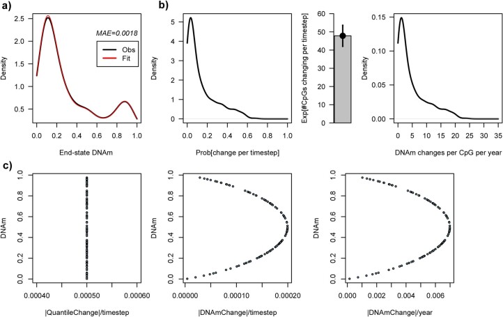
Extended Data Fig. 2 Interpretation of optimal parameter values. a) Density plots of the observed (black) and estimated (red) end-state DNAm-values of the 353 Horvath Clock CpGs, with the median absolute error (MAE) given in the plot. b) Left: Density plot of the estimated probability of change per unit time step for the 353 Horvath CpGs. Middle: Barplot gives the estimated average number of CpGs (+/- standard deviation) that change per timestep. Mean and standard deviation are analytical estimates from a binomial distribution with n = 353. Right: Density plot of the estimated number of DNAm changes a CpG undergoes per year for all 353 CpGs. c) Left: the optimal standard deviation change in the normal quantile basis (x-axis) was estimated to be 5e-4, which is the same irrespective of the actual DNAm-value (y-axis), reflecting the desire to have homoscedastic changes. Middle: corresponding plot when considering the change in the DNAm-value basis, displaying the natural heteroscedasticity of beta-values, as required. Right: as Middle, but now plotting the x-axis on the scale of DNAm change per year, that is the maximum DNAm change per year amounts to about 0.8% (that is 0.008) in units of beta-values.
Extended Data Fig. 2 Interpretation of optimal parameter values. a) Density plots of the observed (black) and estimated (red) end-state DNAm-values of the 353 Horvath Clock CpGs, with the median absolute error (MAE) given in the plot. b) Left: Density plot of the estimated probability of change per unit time step for the 353 Horvath CpGs. Middle: Barplot gives the estimated average number of CpGs (+/- standard deviation) that change per timestep. Mean and standard deviation are analytical estimates from a binomial distribution with n = 353. Right: Density plot of the estimated number of DNAm changes a CpG undergoes per year for all 353 CpGs. c) Left: the optimal standard deviation change in the normal quantile basis (x-axis) was estimated to be 5e-4, which is the same irrespective of the actual DNAm-value (y-axis), reflecting the desire to have homoscedastic changes. Middle: corresponding plot when considering the change in the DNAm-value basis, displaying the natural heteroscedasticity of beta-values, as required. Right: as Middle, but now plotting the x-axis on the scale of DNAm change per year, that is the maximum DNAm change per year amounts to about 0.8% (that is 0.008) in units of beta-values.CC BY · PubMed Central
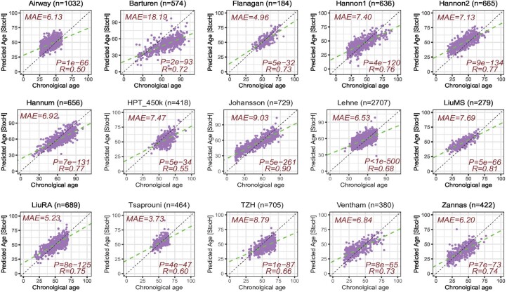
Extended Data Fig. 3 Stochastic Horvath (StocH) clock predicts chronological age in whole blood cohorts. Scatterplots of the true age (x-axis) vs predicted age (y-axis) for the StocH clock in 15 whole blood cohorts. Number of samples in each cohort is indicated above each plot. Median Absolute Error (MAE), R-value and associated nominal correlation-test two-tailed P-value are given.
Extended Data Fig. 3 Stochastic Horvath (StocH) clock predicts chronological age in whole blood cohorts. Scatterplots of the true age (x-axis) vs predicted age (y-axis) for the StocH clock in 15 whole blood cohorts. Number of samples in each cohort is indicated above each plot. Median Absolute Error (MAE), R-value and associated nominal correlation-test two-tailed P-value are given.CC BY · PubMed Central
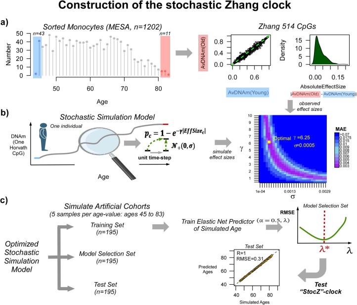
Extended Data Fig. 4 Construction of the Stochastic Zhang (StocZ) clock. a) Left: age distribution of the 1202 sorted monocyte samples from the MESA study, for which Illumina 450k DNAm profiles have been generated. The shaded blue and red regions highlight the youngest and oldest samples that are used in the simulation model. Middle panel displays the average DNAm over the youngest and oldest samples for each of the 514 Zhang Clock CpGs and right panel displays the corresponding density of absolute effect sizes defined as the magnitude of the DNAm difference between youngest and oldest samples. b) The stochastic simulation model of one CpG in one individual of a given age, starts out from the average DNAm in the youngest samples, and subsequently adds a stochastic deviate for each unit time-step. The probability per time-step that a CpG is altered is given by an exponential decaying function with the exponent determined by the observed absolute effect size of the CpG and a CpG-independent parameter, γ, that controls the overall probability of CpGs changing. The direction of the DNAm change is dictated by the directionality of the observed effect size, with the magnitude determined by the standard deviation, σ, of a signed Gaussian distribution, as indicated. Of note, the simulation model adds Gaussian deviates to the quantiles of an inverse Normal distribution, where the DNAm-values are interpreted as probabilities of DNAm. The model is simulated to generate effect sizes for each of the 514 Zhang clock CpGs, which is then compared to the observed distribution to identify the optimal (λ,σ) parameters that minimize the median absolute error (MAE) between simulated and observed values. c) To build the stochastic Zhang clock, we then use the simulation model with the optimal (λ,σ) parameter values to generate 3 artificial cohorts of 195 samples each. There are 195 samples, because we simulate 5 samples per age-value with ages ranging between 45 and 83 that is a total of 39 distinct age-values. One cohort is used to train Elastic Net Regression models with α = 0.5, and for varying penalty parameter values λ. These models are then evaluated in the model selection set to select the model that optimizes the root mean square error (RMSE). This optimal model is then evaluated in the test set.
Extended Data Fig. 4 Construction of the Stochastic Zhang (StocZ) clock. a) Left: age distribution of the 1202 sorted monocyte samples from the MESA study, for which Illumina 450k DNAm profiles have been generated. The shaded blue and red regions highlight the youngest and oldest samples that are used in the simulation model. Middle panel displays the average DNAm over the youngest and oldest samples for each of the 514 Zhang Clock CpGs and right panel displays the corresponding density of absolute effect sizes defined as the magnitude of the DNAm difference between youngest and oldest samples. b) The stochastic simulation model of one CpG in one individual of a given age, starts out from the average DNAm in the youngest samples, and subsequently adds a stochastic deviate for each unit time-step. The probability per time-step that a CpG is altered is given by an exponential decaying function with the exponent determined by the observed absolute effect size of the CpG and a CpG-independent parameter, γ, that controls the overall probability of CpGs changing. The direction of the DNAm change is dictated by the directionality of the observed effect size, with the magnitude determined by the standard deviation, σ, of a signed Gaussian distribution, as indicated. Of note, the simulation model adds Gaussian deviates to the quantiles of an inverse Normal distribution, where the DNAm-values are interpreted as probabilities of DNAm. The model is simulated to generate effect sizes for each of the 514 Zhang clock CpGs, which is then compared to the observed distribution to identify the optimal (λ,σ) parameters that minimize the median absolute error (MAE) between simulated and observed values. c) To build the stochastic Zhang clock, we then use the simulation model with the optimal (λ,σ) parameter values to generate 3 artificial cohorts of 195 samples each. There are 195 samples, because we simulate 5 samples per age-value with ages ranging between 45 and 83 that is a total of 39 distinct age-values. One cohort is used to train Elastic Net Regression models with α = 0.5, and for varying penalty parameter values λ. These models are then evaluated in the model selection set to select the model that optimizes the root mean square error (RMSE). This optimal model is then evaluated in the test set.CC BY · PubMed Central
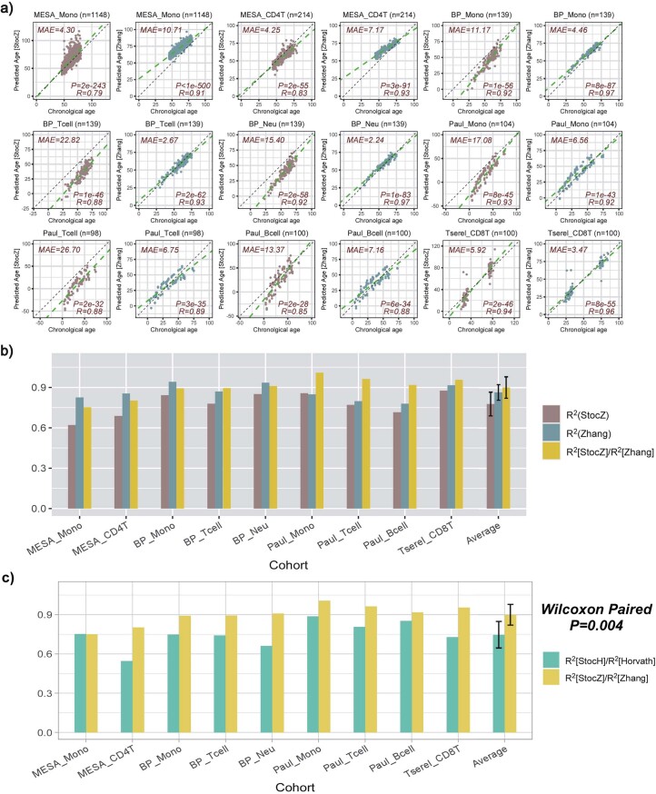
Extended Data Fig. 5 Quantification of the stochastic component of Zhang’s clock in sorted immune cell sets. a) Scatterplots of predicted age vs true age for the StocZ-clock (brown) and Zhang’s clock (green) in sorted immune cell datasets. Number of sorted samples in dataset is indicated at the top of the panel alongside the name of the cohort/study. In addition, we provide the median absolute error (MAE), R-value and corresponding nominal correlation-test two-tailed P-value. b) Barplot comparing R2 values of the StocZ-clock and Zhang’s clock in each of the datasets. We also depict the ratio of the R2 value from StocZ to the R2 value from Zhang’s clock. Sample sizes are: MESA_Mono (n = 1148), MESA_CD4T (n = 214), BP_Mono (n = 139), BP_Tcell (n = 139), BP_Neu (n = 139), Paul_Mono (n = 104), Paul_Tcell (n = 98), Paul_Bcell (n = 100), Tserel_CD8T (n = 100).The last set of bars displays the average and standard deviation over all sorted immune cell datasets. c) Comparison of the ratio of R2 values between Horvath and Zhang CpGs. P-value is from a one-tailed paired Wilcoxon rank sum test comparing the ratio of R2 values. Sample sizes as in b). The last set of bars displays the average and standard deviation over all sorted immune cell datasets.
Extended Data Fig. 5 Quantification of the stochastic component of Zhang’s clock in sorted immune cell sets. a) Scatterplots of predicted age vs true age for the StocZ-clock (brown) and Zhang’s clock (green) in sorted immune cell datasets. Number of sorted samples in dataset is indicated at the top of the panel alongside the name of the cohort/study. In addition, we provide the median absolute error (MAE), R-value and corresponding nominal correlation-test two-tailed P-value. b) Barplot comparing R2 values of the StocZ-clock and Zhang’s clock in each of the datasets. We also depict the ratio of the R2 value from StocZ to the R2 value from Zhang’s clock. Sample sizes are: MESA_Mono (n = 1148), MESA_CD4T (n = 214), BP_Mono (n = 139), BP_Tcell (n = 139), BP_Neu (n = 139), Paul_Mono (n = 104), Paul_Tcell (n = 98), Paul_Bcell (n = 100), Tserel_CD8T (n = 100).The last set of bars displays the average and standard deviation over all sorted immune cell datasets. c) Comparison of the ratio of R2 values between Horvath and Zhang CpGs. P-value is from a one-tailed paired Wilcoxon rank sum test comparing the ratio of R2 values. Sample sizes as in b). The last set of bars displays the average and standard deviation over all sorted immune cell datasets.CC BY · PubMed Central
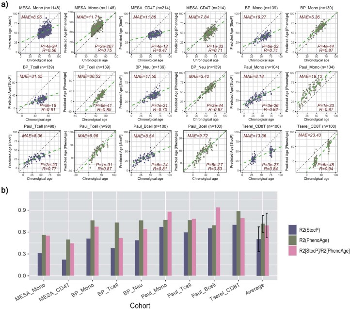
Extended Data Fig. 6 Quantifying stochastic component of PhenoAge-clock in sorted immune cell datasets. a) Scatterplots of predicted age vs chronological (true) age for the stochastic PhenoAge-clock (StocP) in sorted immune-cell datasets. Number of samples in dataset is indicated at the top of the panel alongside the name of the cohort/study. In addition, we provide the median absolute error (MAE), R-value and corresponding nominal correlation-test two-tailed P-value. b) R2 values for StocP, PhenoAge clock and their ratio across all datasets. Sample sizes are: MESA_Mono (n = 1148), MESA_CD4T (n = 214), BP_Mono (n = 139), BP_Tcell (n = 139), BP_Neu (n = 139), Paul_Mono (n = 104), Paul_Tcell (n = 98), Paul_Bcell (n = 100), Tserel_CD8T (n = 100). The last set of bars displays the average and standard deviation over all sorted immune cell datasets.
Extended Data Fig. 6 Quantifying stochastic component of PhenoAge-clock in sorted immune cell datasets. a) Scatterplots of predicted age vs chronological (true) age for the stochastic PhenoAge-clock (StocP) in sorted immune-cell datasets. Number of samples in dataset is indicated at the top of the panel alongside the name of the cohort/study. In addition, we provide the median absolute error (MAE), R-value and corresponding nominal correlation-test two-tailed P-value. b) R2 values for StocP, PhenoAge clock and their ratio across all datasets. Sample sizes are: MESA_Mono (n = 1148), MESA_CD4T (n = 214), BP_Mono (n = 139), BP_Tcell (n = 139), BP_Neu (n = 139), Paul_Mono (n = 104), Paul_Tcell (n = 98), Paul_Bcell (n = 100), Tserel_CD8T (n = 100). The last set of bars displays the average and standard deviation over all sorted immune cell datasets.CC BY · PubMed Central
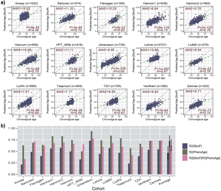
Extended Data Fig. 7 Quantifying stochastic component of PhenoAge-clock in whole blood datasets. a) Scatterplots of predicted age vs chronological (true) age for the stochastic PhenoAge-clock (StocP) in whole blood datasets. Number of samples in dataset is indicated at the top of the panel alongside the name of the cohort/study. In addition, we provide the median absolute error (MAE), R-value and corresponding nominal correlation-test two-tailed P-value. b) R2 values for StocP, PhenoAge clock and their ratio across all datasets. Sample sizes are: Airway (n = 1032), Barturen (n = 574), Flanagan (n = 184), Hannon1 (n = 636), Hannon2 (n = 665), Hannum (n = 656), HPT_450k (n = 418), Johansson (n = 729), Lehne (n = 2707), LiuMS (n = 279), LiuRA (n = 689), Tsaprouni (n = 464), TZH (n = 705), Ventham (n = 380), Zannas (n = 422). The last set of bars displays the average and standard deviation over all whole blood datasets.
Extended Data Fig. 7 Quantifying stochastic component of PhenoAge-clock in whole blood datasets. a) Scatterplots of predicted age vs chronological (true) age for the stochastic PhenoAge-clock (StocP) in whole blood datasets. Number of samples in dataset is indicated at the top of the panel alongside the name of the cohort/study. In addition, we provide the median absolute error (MAE), R-value and corresponding nominal correlation-test two-tailed P-value. b) R2 values for StocP, PhenoAge clock and their ratio across all datasets. Sample sizes are: Airway (n = 1032), Barturen (n = 574), Flanagan (n = 184), Hannon1 (n = 636), Hannon2 (n = 665), Hannum (n = 656), HPT_450k (n = 418), Johansson (n = 729), Lehne (n = 2707), LiuMS (n = 279), LiuRA (n = 689), Tsaprouni (n = 464), TZH (n = 705), Ventham (n = 380), Zannas (n = 422). The last set of bars displays the average and standard deviation over all whole blood datasets.CC BY · PubMed Central
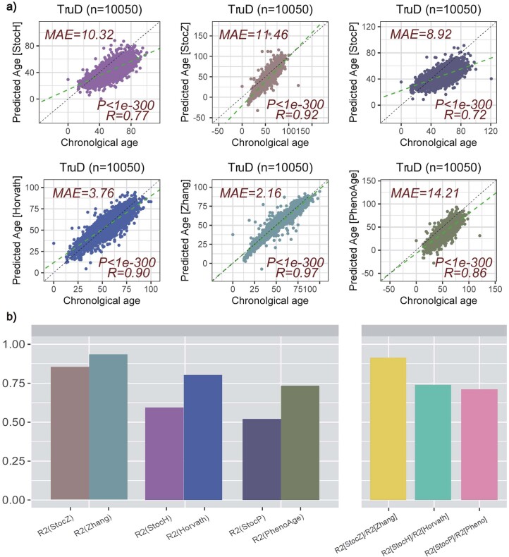
Extended Data Fig. 8 Quantification of stochastic aging component in TruD cohort. a) Scatterplot of predicted age vs chronological age for the 3 stochastic clocks (StocH, StocZ and StocP, top row) and their original clocks (Horvath, Zhang and PhenoAge, bottom row). In each case, we provide the MAE, R and nominal correlation-test two-tailed P-value. b) Barplot comparing the R2 values of the 6 clocks (left) and the ratio of R2 values (right).
Extended Data Fig. 8 Quantification of stochastic aging component in TruD cohort. a) Scatterplot of predicted age vs chronological age for the 3 stochastic clocks (StocH, StocZ and StocP, top row) and their original clocks (Horvath, Zhang and PhenoAge, bottom row). In each case, we provide the MAE, R and nominal correlation-test two-tailed P-value. b) Barplot comparing the R2 values of the 6 clocks (left) and the ratio of R2 values (right).CC BY · PubMed Central
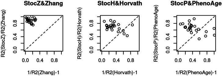
Extended Data Fig. 9 Stochastic clocks do not describe the unexplained age-variation of epigenetic clocks. Scatterplot of RR2 measures (y-axis) against 1/R2 – 1 (x-axis) for each clock-type, with the line of proportionality shown as a dashed line.
Extended Data Fig. 9 Stochastic clocks do not describe the unexplained age-variation of epigenetic clocks. Scatterplot of RR2 measures (y-axis) against 1/R2 – 1 (x-axis) for each clock-type, with the line of proportionality shown as a dashed line.CC BY · PubMed Central
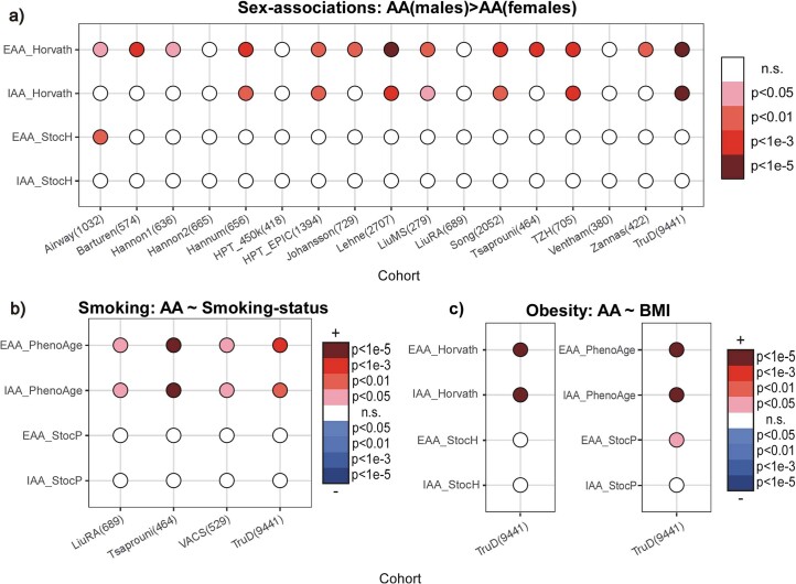
Extended Data Fig. 10 Stochastic clocks display reduced age-accelerations with sex, smoking and obesity. a) Balloon plot depicting associations of extrinsic and intrinsic age acceleration (EAA & IAA) with sex for the Horvath and StocH-clocks across 17 whole blood cohorts with available sex information. P-values derive from a one-tailed Wilcoxon rank sum test, with the alternative hypothesis being higher age-acceleration (AA) in males. b) Balloon plot depicting associations of extrinsic and intrinsic age acceleration (EAA & IAA) with smoking status for the PhenoAge and StocP-clocks across 4 whole blood cohorts with smoking information and where associations with smoking-status were found. P-value derives from a two-tailed correlation test. In the color-legend, + means higher AA in smokers. c) Balloon plot depicting associations of extrinsic and intrinsic age acceleration (EAA & IAA) with body-mass-index (BMI) for the Horvath/StocH and PhenoAge/StocP-clocks in the TruD cohort where an association of AA with BMI was found. P-value derives from a two-tailed correlation test. In the color-legend, + means higher AA in smokers.
Extended Data Fig. 10 Stochastic clocks display reduced age-accelerations with sex, smoking and obesity. a) Balloon plot depicting associations of extrinsic and intrinsic age acceleration (EAA & IAA) with sex for the Horvath and StocH-clocks across 17 whole blood cohorts with available sex information. P-values derive from a one-tailed Wilcoxon rank sum test, with the alternative hypothesis being higher age-acceleration (AA) in males. b) Balloon plot depicting associations of extrinsic and intrinsic age acceleration (EAA & IAA) with smoking status for the PhenoAge and StocP-clocks across 4 whole blood cohorts with smoking information and where associations with smoking-status were found. P-value derives from a two-tailed correlation test. In the color-legend, + means higher AA in smokers. c) Balloon plot depicting associations of extrinsic and intrinsic age acceleration (EAA & IAA) with body-mass-index (BMI) for the Horvath/StocH and PhenoAge/StocP-clocks in the TruD cohort where an association of AA with BMI was found. P-value derives from a two-tailed correlation test. In the color-legend, + means higher AA in smokers.CC BY · PubMed Central

Verification

Claims the paper makes

The claims and statistics of this paper haven’t been checked yet.

Run the check — free, no account needed. It reads the open-access text and checks the sources it cites.

A few free checks a day · papers already verified open instantly · results are public

Claims other papers make about this one

Each is checked against this paper’s own text: does it say what the citing paper says it does?

Self-check

Percentages, sums and reported differences re-computed from the paper’s own numbers.

The self-check needs the paper’s full text.

Citations

Cites

Show all 14 references

Research works printed but not linked: 62

  1. Vijg, J. From DNA damage to mutations: all roads lead to aging. Ageing Res. Rev. 68, 101316 (2021). · DOI
  2. Laurie, C. C. et al. Detectable clonal mosaicism from birth to old age and its relationship to cancer. Nat. Genet. 44, 642–650 (2012). · DOI · Paper page
  3. Jacobs, K. B. et al. Detectable clonal mosaicism and its relationship to aging and cancer. Nat. Genet. 44, 651–658 (2012). · DOI · Paper page
  4. Ahuja, N. & Issa, J. P. Aging, methylation and cancer. Histol. Histopathol. 15, 835–842 (2000).
  5. Ahuja, N., Li, Q., Mohan, A. L., Baylin, S. B. & Issa, J. P. Aging and DNA methylation in colorectal mucosa and cancer. Cancer Res. 58, 5489–5494 (1998).
  6. Issa, J. P., Ahuja, N., Toyota, M., Bronner, M. P. & Brentnall, T. A. Accelerated age-related CpG island methylation in ulcerative colitis. Cancer Res. 61, 3573–3577 (2001).
  7. Christensen, B. C. et al. Aging and environmental exposures alter tissue-specific DNA methylation dependent upon CpG island context. PLoS Genet. 5, e1000602 (2009). · DOI
  8. de Magalhaes, J. P. Ageing as a software design flaw. Genome Biol. 24, 51 (2023). · DOI
  9. Teschendorff, A. E. et al. An epigenetic signature in peripheral blood predicts active ovarian cancer. PLoS ONE 4, e8274 (2009). · DOI
  10. Teschendorff, A. E. et al. Age-dependent DNA methylation of genes that are suppressed in stem cells is a hallmark of cancer. Genome Res. 20, 440–446 (2010). · DOI · Paper page
  11. Rakyan, V. K. et al. Human aging-associated DNA hypermethylation occurs preferentially at bivalent chromatin domains. Genome Res. 20, 434–439 (2010). · DOI
  12. Hannum, G. et al. Genome-wide methylation profiles reveal quantitative views of human aging rates. Mol. Cell 49, 359–367 (2013). · DOI · Paper page
  13. Horvath, S. & Raj, K. DNA methylation-based biomarkers and the epigenetic clock theory of ageing. Nat. Rev. Genet. 19, 371–384 (2018). · DOI · Paper page
  14. Marioni, R. E. et al. DNA methylation age of blood predicts all-cause mortality in later life. Genome Biol. 16, 25 (2015). · DOI · Paper page
  15. Levine, M. E. et al. DNA methylation age of blood predicts future onset of lung cancer in the women’s health initiative. Aging 7, 690–700 (2015). · DOI
  16. Levine, M. E. et al. An epigenetic biomarker of aging for lifespan and healthspan. Aging 10, 573–591 (2018). · DOI · Paper page
  17. Seale, K., Horvath, S., Teschendorff, A., Eynon, N. & Voisin, S. Making sense of the ageing methylome. Nat. Rev. Genet. 23, 585–605 (2022). · DOI · Paper page
  18. West, J., Beck, S., Wang, X. & Teschendorff, A. E. An integrative network algorithm identifies age-associated differential methylation interactome hotspots targeting stem-cell differentiation pathways. Sci. Rep. 3, 1630 (2013). · DOI
  19. West, J., Widschwendter, M. & Teschendorff, A. E. Distinctive topology of age-associated epigenetic drift in the human interactome. Proc. Natl Acad. Sci. USA 110, 14138–14143 (2013). · DOI
  20. Nejman, D. et al. Molecular rules governing de novo methylation in cancer. Cancer Res. 74, 1475–1483 (2014). · DOI
  21. Maegawa, S. et al. Widespread and tissue specific age-related DNA methylation changes in mice. Genome Res. 20, 332–340 (2010). · DOI · Paper page
  22. Slieker, R. C. et al. Age-related accrual of methylomic variability is linked to fundamental ageing mechanisms. Genome Biol. 17, 191 (2016). · DOI
  23. Tarkhov, A. E. et al. Nature of epigenetic aging from a single-cell perspective. Preprint at https://www.biorxiv.org/content/10.1101/2022.09.26.509592v2 (2022). · DOI
  24. Minteer, C. J. et al. More than bad luck: cancer and aging are linked to replication-driven changes to the epigenome. Sci. Adv. 9, eadf4163 (2023). · DOI
  25. Vandiver, A. R. et al. Age and sun exposure-related widespread genomic blocks of hypomethylation in nonmalignant skin. Genome Biol. 16, 80 (2015). · DOI
  26. Poganik, J. R. et al. Biological age is increased by stress and restored upon recovery. Cell Metab. 35, 807–820 e5 (2023). · DOI · Paper page
  27. Reynolds, L. M. et al. Tobacco exposure-related alterations in DNA methylation and gene expression in human monocytes: the Multi-Ethnic Study of Atherosclerosis (MESA). Epigenetics 12, 1092–1100 (2017). · DOI
  28. Teschendorff, A. E. A comparison of epigenetic mitotic-like clocks for cancer risk prediction. Genome Med. 12, 56 (2020). · DOI
  29. Friedman, J., Hastie, T. & Tibshirani, R. Regularization paths for generalized linear models via coordinate descent. J. Stat. Softw. 33, 1–22 (2010). · DOI · Paper page
  30. Chen, L. et al. Genetic drivers of epigenetic and transcriptional variation in human immune cells. Cell 167, 1398–1414 e24 (2016). · DOI · Paper page
  31. Luo, Q. et al. A meta-analysis of immune-cell fractions at high resolution reveals novel associations with common phenotypes and health outcomes. Genome Med. 15, 59 (2023). · DOI
  32. Cao, X. et al. Accelerated biological aging in COVID-19 patients. Nat. Commun. 13, 2135 (2022). · DOI
  33. Barturen, G. et al. Whole blood DNA methylation analysis reveals respiratory environmental traits involved in COVID-19 severity following SARS-CoV-2 infection. Nat. Commun. 13, 4597 (2022). · DOI
  34. Kim, J. Y., Tavare, S. & Shibata, D. Counting human somatic cell replications: methylation mirrors endometrial stem cell divisions. Proc. Natl Acad. Sci. USA 102, 17739–17744 (2005). · DOI
  35. Siegmund, K. D., Marjoram, P., Woo, Y. J., Tavare, S. & Shibata, D. Inferring clonal expansion and cancer stem cell dynamics from DNA methylation patterns in colorectal cancers. Proc. Natl Acad. Sci. USA 106, 4828–4833 (2009). · DOI
  36. Tomasetti, C. & Vogelstein, B. Cancer etiology. Variation in cancer risk among tissues can be explained by the number of stem cell divisions. Science 347, 78–81 (2015). · DOI · Paper page
  37. Jonkman, T. H. et al. Functional genomics analysis identifies T and NK cell activation as a driver of epigenetic clock progression. Genome Biol. 23, 24 (2022). · DOI
  38. Joehanes, R. et al. Epigenetic signatures of cigarette smoking. Circ. Cardiovasc. Genet. 9, 436–447 (2016). · DOI
  39. You, C. et al. A cell-type deconvolution meta-analysis of whole blood EWAS reveals lineage-specific smoking-associated DNA methylation changes. Nat. Commun. 11, 4779 (2020). · DOI
  40. Teschendorff, A. E. et al. Correlation of smoking-associated DNA methylation changes in buccal cells with DNA methylation changes in epithelial cancer. JAMA Oncol. 1, 476–485 (2015). · DOI
  41. van Dongen, J. et al. Effects of smoking on genome-wide DNA methylation profiles: a study of discordant and concordant monozygotic twin pairs. eLife 12, e83286 (2023). · DOI
  42. Endicott, J. L., Nolte, P. A., Shen, H. & Laird, P. W. Cell division drives DNA methylation loss in late-replicating domains in primary human cells. Nat. Commun. 13, 6659 (2022). · DOI
  43. Gao, Y. et al. The integrative epigenomic-transcriptomic landscape of ER-positive breast cancer. Clin. Epigenetics 7, 126 (2015). · DOI
  44. Chen, Y., Breeze, C. E., Zhen, S., Beck, S. & Teschendorff, A. E. Tissue-independent and tissue-specific patterns of DNA methylation alteration in cancer. Epigenetics Chromatin 9, 10 (2016). · DOI
  45. Zhu, L. et al. Multi-organ mapping of cancer risk. Cell 166, 1132–1146 e7 (2016). · DOI
  46. Levine, M.E., Higgins-Chen, A., Thrush, K., Minteer, C. & Niimi, P. Clock work: deconstructing epigenetic clock signals in aging, disease and reprogramming. Preprint at bioRxiv https://doi.org/10.1101/2022.02.13.480245 (2023). · DOI
  47. Martin-Herranz, D. E. et al. Screening for genes that accelerate the epigenetic aging clock in humans reveals a role for the H3K36 methyltransferase NSD1. Genome Biol. 20, 146 (2019). · DOI
  48. Reynolds, L. M. et al. Age-related variations in the methylome associated with gene expression in human monocytes and T cells. Nat. Commun. 5, 5366 (2014). · DOI
  49. Tserel, L. et al. Age-related profiling of DNA methylation in CD8+ T cells reveals changes in immune response and transcriptional regulator genes. Sci. Rep. 5, 13107 (2015). · DOI
  50. Paul, D. S. et al. Increased DNA methylation variability in type 1 diabetes across three immune effector cell types. Nat. Commun. 7, 13555 (2016). · DOI
  51. Norris, J.R. Markov Chains (Cambridge Univ. Press, 1997). · DOI
  52. Teschendorff, A. E. Avoiding common pitfalls in machine learning omic data science. Nat. Mater. 18, 422–427 (2019). · DOI · Paper page
  53. Pelegi-Siso, D., de Prado, P., Ronkainen, J., Bustamante, M. & Gonzalez, J. R. methylclock: a Bioconductor package to estimate DNA methylation age. Bioinformatics 37, 1759–1760 (2021). · DOI
  54. Teschendorff, A. E., Breeze, C. E., Zheng, S. C. & Beck, S. A comparison of reference-based algorithms for correcting cell-type heterogeneity in epigenome-wide association studies. BMC Bioinform. 18, 105 (2017). · DOI
  55. Zheng, S.C. et al. EpiDISH web server: epigenetic dissection of intra-sample-heterogeneity with online GUI. Bioinformatics 36, 1950–1951 (2019). · DOI
  56. Johnson, K. C. et al. DNA methylation in ductal carcinoma in situ related with future development of invasive breast cancer. Clin. Epigenetics 7, 75 (2015). · DOI
  57. Troyanskaya, O. et al. Missing value estimation methods for DNA microarrays. Bioinformatics 17, 520–525 (2001). · DOI · Paper page
  58. Huang, K. K. et al. Genomic and epigenomic profiling of high-risk intestinal metaplasia reveals molecular determinants of progression to gastric cancer. Cancer Cell 33, 137–150 e5 (2018). · DOI
  59. Luebeck, E. G. et al. Identification of a key role of widespread epigenetic drift in Barrett’s esophagus and esophageal adenocarcinoma. Clin. Epigenetics 9, 113 (2017). · DOI
  60. Maity, A. K. et al. Novel epigenetic network biomarkers for early detection of esophageal cancer. Clin. Epigenetics 14, 23 (2022). · DOI
  61. Bormann, F. et al. Cell-of-origin DNA methylation signatures are maintained during colorectal carcinogenesis. Cell Rep. 23, 3407–3418 (2018). · DOI
  62. Teschendorff, A. E. et al. DNA methylation outliers in normal breast tissue identify field defects that are enriched in cancer. Nat. Commun. 7, 10478 (2016). · DOI

Cited by

Sorted by citations

Metadata

Authors
Tong, H., Dwaraka, V. B., Chen, Q., Luo, Q., Lasky-Su, J. A., Smith, R., & Teschendorff, A. E.
Venue
Nature Aging
Published
2024-05-09
Volume
4
Issue
6
Pages
886-901
ISSN
2662-8465
Cited by
83
References
14
Language
en
Funders
National Natural Science Foundation of China (32370699, 32170652, 31970632)

About these checks

Registry, retraction, Cites and statistics results are computed, not judged, with one exception: a printed reference that no index lists is read once by a model before it counts as a citation error. Claims are extracted by a model and kept only when their quote appears verbatim in the text; each cited source is then checked, with a model’s help, for whether it says what the claim relies on. Those verdicts can be wrong — read the claim’s quote and the cited source before relying on one.

Statistics and arithmetic are recomputed, not judged.

Confidence bands are shown only for fields calibrated on our annotated test set. None is calibrated yet, so no band is shown.

What counts as a claim ›How we measure confidence ›How we check this ›

Are you an author, or do you see a problem with this page? Request a review