

Solving Quantum Ground-State Problems with Nuclear Magnetic Resonance
Open accessThe DOI matches its Crossref record; 37 of the 38 references it cites were found in a registry or an index.
Abstract
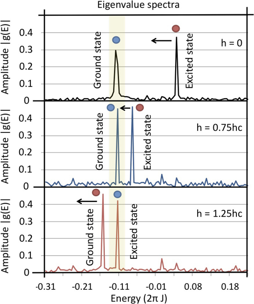
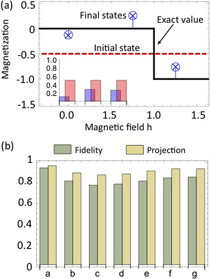
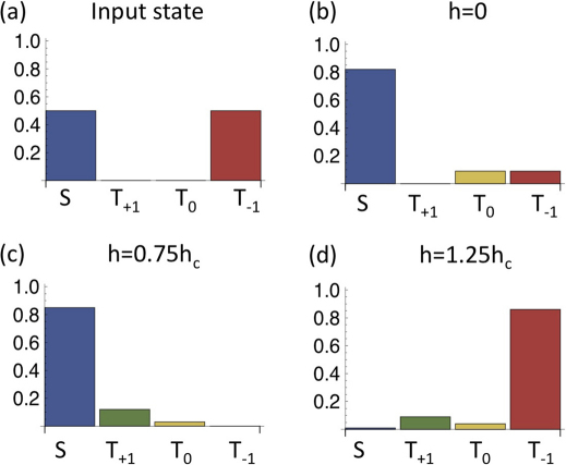
Quantum ground-state problems are computationally hard problems for general many-body Hamiltonians; there is no classical or quantum algorithm known to be able to solve them efficiently. Nevertheless, if a trial wavefunction approximating the ground state is available, as often happens for many problems in physics and chemistry, a quantum computer could employ this trial wavefunction to project the ground state by means of the phase estimation algorithm (PEA). We performed an experimental realization of this idea by implementing a variational-wavefunction approach to solve the ground-state problem of the Heisenberg spin model with an NMR quantum simulator. Our iterative phase estimation procedure yields a high accuracy for the eigenenergies (to the 10⁻⁵ decimal digit). The ground-state fidelity was distilled to be more than 80%, and the singlet-to-triplet switching near the critical field is reliably captured. This result shows that quantum simulators can better leverage classical trial wave functions than classical computers.
Overview
The claims and statistics of this paper haven’t been checked yet.
Free: it reads the open-access text and checks the first 5 claims that cite a source we can check. Create a free account to check every claim.
Integrity signals
Registry
Cites
Statistics
Figures




Verification
Claims the paper makes
The claims and statistics of this paper haven’t been checked yet.
Free: it reads the open-access text and checks the first 5 claims that cite a source we can check. Create a free account to check every claim.
Claims other papers make about this one
Each is checked against this paper’s own text: does it say what the citing paper says it does?
The source backs part of the claim, not all of it — or backs it for a different population, condition or comparison.
In the citing paper
“In fact, locating these eigenvalues can be achieved by the phase estimation method utilizing one extra ancilla qubit12 corresponding, in our case, to one additional ion.”
From From transistor to trapped-ion computers for quantum chemistry (2014) · cites this paper as [12]
Experimental — accuracy not yet measured
Self-check
Percentages, sums and reported differences re-computed from the paper’s own numbers.
The self-check needs the paper’s full text.
Citations
Cites
Simulating physics with computers
Feynman, R. P. (1982) · International Journal of Theoretical Physics · doi:10.1007/bf02650179 · Cited by 7,691
Ladd, T. D., Jelezko, F., Laflamme, R., Nakamura, Y., Monroe, C., & O’Brien, J. L. (2010) · Nature · doi:10.1038/nature08812 · Cited by 3,592
Solution of the Schrödinger equation by a spectral method
Feit, M. D., Fleck, J. A., & Steiger, A. (1982) · Journal of Computational Physics · doi:10.1016/0021-9991(82)90091-2 · Cited by 3,368
Nobel Lecture: Electronic structure of matter—wave functions and density functionals
Kohn, W. (1999) · Reviews of Modern Physics · doi:10.1103/revmodphys.71.1253 · Cited by 2,637
Molecular Electronic‐Structure Theory
Helgaker, T., Jørgensen, P., & Olsen, J. (2000) · doi:10.1002/9781119019572 · Cited by 2,594
Brucker, P. (1995) · Scheduling Algorithms · doi:10.1007/978-3-662-03088-2_3 · Cited by 2,289
Molecular electronic-structure theory
Ratner, M. A. (2000) · Cited by 1,565
Simulated Quantum Computation of Molecular Energies
Aspuru-Guzik, A., Dutoi, A. D., Love, P. J., & Head-Gordon, M. (2005) · Science · doi:10.1126/science.1113479 · Cited by 1,418
Self-citationClassical and Quantum Computation
Kitaev, A., Shen, A., & Vyalyi, M. (2002) · Graduate Studies in Mathematics · doi:10.1090/gsm/047 · Cited by 1,387
On the computational complexity of Ising spin glass models
Barahona, F. (1982) · Journal of Physics A: Mathematical and General · doi:10.1088/0305-4470/15/10/028 · Cited by 1,306 · cited 1×
“The Ising model with nonuniform couplings is an example of an NP -problem (more precisely, NP -complete”
Method
Cited by
Georgescu, I. M., Ashhab, S., & Nori, F. (2014) · Reviews of Modern Physics · doi:10.1103/revmodphys.86.153 · Cited by 2,932
“Nuclear spins manipulated by means of NMR have been among the first experimental systems to implement small quantum algorithms and quantum simulation (Li et al., 2011; Peng and Suter, 2010; Peng et al., 2009; Zhang et al., 2012).”
MethodQuantum computational chemistry
McArdle, S., Endo, S., Aspuru-Guzik, A., Benjamin, S. C., & Yuan, X. (2020) · Reviews of Modern Physics · doi:10.1103/revmodphys.92.015003 · Cited by 1,621
Self-citationThe Variational Quantum Eigensolver: A review of methods and best practices
Tilly, J., Chen, H., Cao, S., Picozzi, D., Setia, K., Li, Y., Grant, E., Wossnig, L., Rungger, I., Booth, G. H., et al. (2022) · Physics Reports · doi:10.1016/j.physrep.2022.08.003 · Cited by 1,031
Self-citationQuantum optimization using variational algorithms on near-term quantum devices
Moll, N., Barkoutsos, P., Bishop, L. S., Chow, J. M., Cross, A., Egger, D. J., Filipp, S., Fuhrer, A., Gambetta, J. M., Ganzhorn, M., et al. (2018) · Quantum Science and Technology · doi:10.1088/2058-9565/aab822 · Cited by 744
Quantum Chemistry Calculations on a Trapped-Ion Quantum Simulator
Hempel, C., Maier, C., Romero, J., McClean, J., Monz, T., Shen, H., Jurcevic, P., Lanyon, B. P., Love, P., Babbush, R., et al. (2018) · Physical Review X · doi:10.1103/physrevx.8.031022 · Cited by 446
“[89] Zhaokai Li, Man-Hong Yung, Hongwei Chen, Danwei Lu, James D.”
MethodSelf-citation
Metadata
- Authors
- Li, Z., Yung, M.-H., Chen, H., Lu, D., Whitfield, J. D., Peng, X., Aspuru-Guzik, A., & Du, J.
- Affiliations
- University of Science and Technology of China (CN)
- Harvard University (US)
- Corresponding author
- Du, Jiangfeng
- Venue
- Scientific Reports
- Published
- 2011-09-09
- Volume
- 1
- Issue
- 1
- Pages
- 88-88
- ISSN
- 2045-2322 (ISSN-L)
- PMC
- PMC3216574
- OpenAlex
- W2034692119
- Cited by
- 63
- References
- 38
- Citations by year
- 2026: 2 · 2024: 4 · 2023: 3 · 2022: 8 · 2021: 2 · 2020: 10 · 2019: 2 · 2018: 6 · 2017: 4 · 2016: 3 · 2015: 3 · 2014: 7 · 2013: 2 · 2012: 7
- FWCI
- 4.71
- Type
- journal article
- Language
- en
- Update notices
- erratum (2012-11-29)
- Open access
- gold
- doi.org
- Licence
- cc-by-nc-nd
- creativecommons.org/licenses/by-nc-nd/3.0/ (tdm)
- creativecommons.org/licenses/by-nc-nd/3.0/ (vor)
- Locations
- Scientific Reports (publishedVersion, cc-by-nc-nd)
- PubMed Central (publishedVersion, cc-by-nc-nd)
- PubMed (publishedVersion)
- arXiv (Cornell University) (submittedVersion)
- Digital Access to Scholarship at Harvard (DASH) (Harvard University) (submittedVersion, cc-by)
- arXiv (Cornell University)
- Funders
- National Science Foundation (1037992)
- U.S. Department of Defense
- Alfred P. Sloan Foundation
- Camille and Henry Dreyfus Foundation
- Croucher Foundation
- National Natural Science Foundation of China
- Defense Advanced Research Projects Agency (N66001)
- Division of Chemistry (CHE-1037992)
- Topics
- Physical Sciences › Computer Science › Artificial Intelligence › Quantum Computing Algorithms and Architecture
- Physical Sciences › Physics and Astronomy › Atomic and Molecular Physics, and Optics › Quantum many-body systems
- Physical Sciences › Physics and Astronomy › Atomic and Molecular Physics, and Optics › Quantum Information and Cryptography
- Keywords
- variational quantum eigensolver, Heisenberg model, trial wave functions, ground-state fidelity, singlet-triplet transitions
About these checks
Registry, retraction, Cites and statistics results are computed, not judged, with one exception: a printed reference that no index lists is read once by a model before it counts as a citation error. Claims are extracted by a model and kept only when their quote appears verbatim in the text; each cited source is then checked, with a model’s help, for whether it says what the claim relies on. Those verdicts can be wrong — read the claim’s quote and the cited source before relying on one.
Statistics and arithmetic are recomputed, not judged.
Confidence bands are shown only for fields calibrated on our annotated test set. None is calibrated yet, so no band is shown.
What counts as a claim ›How we measure confidence ›How we check this ›
Are you an author, or do you see a problem with this page? Request a review
How to cite
Cite CoChat for the checks on this page, and the paper for its own findings.
- This page
- CoChat. (2026). Citation check: Solving Quantum Ground-State Problems with Nuclear Magnetic Resonance. https://app.cochat.ai/papers/10.1038/srep00088
- The paper
- Li, Z., Yung, M.-H., Chen, H., Lu, D., Whitfield, J. D., Peng, X., Aspuru-Guzik, A., & Du, J. (2011). Solving Quantum Ground-State Problems with Nuclear Magnetic Resonance. Scientific Reports. https://doi.org/10.1038/srep00088
Data sources
Bibliographic data: Semantic Scholar, OpenAlex, Crossref.
Contains information from the Semantic Scholar Academic Graph Datasets, made available under the ODC Attribution License (ODC-BY 1.0).
Semantic Scholar’s data is described in: Kinney, R., et al. (2023). The Semantic Scholar Open Data Platform. arXiv:2301.10140.
