

The DOI matches its Crossref record; 14 of the 14 references it cites were found in a registry or an index.
Investigating Population History Using Temporal Genetic Differentiation
Overview
The claims and statistics of this paper haven’t been checked yet.
Run the check — free, no account needed. It reads the open-access text and checks the sources it cites.
Integrity signals
Registry
Cites
Statistics
Figures
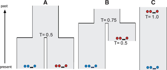
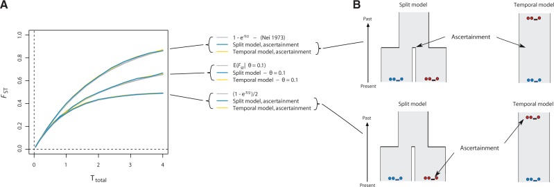
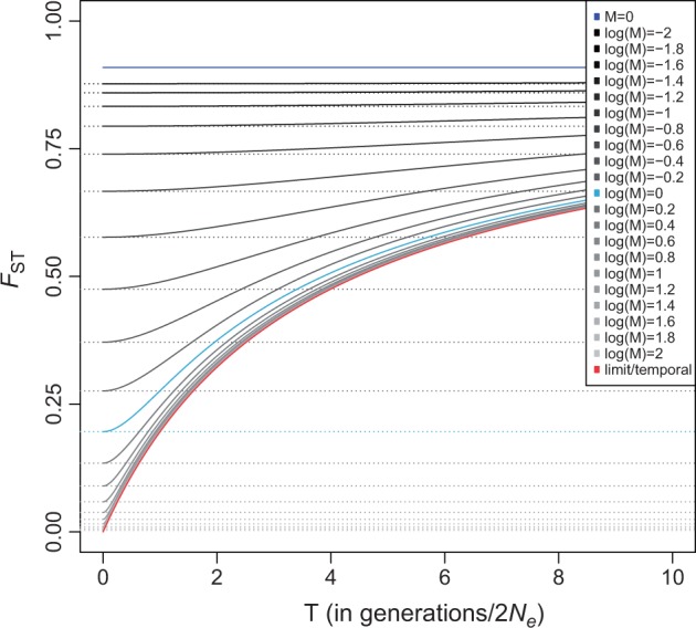
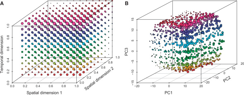
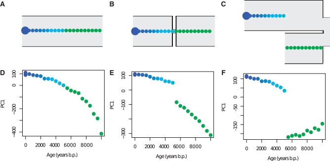
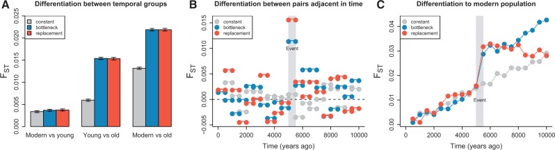
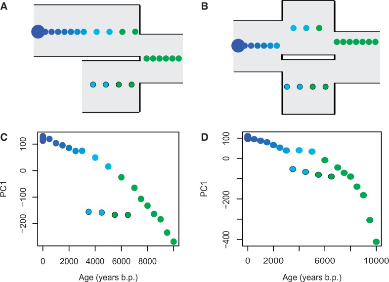
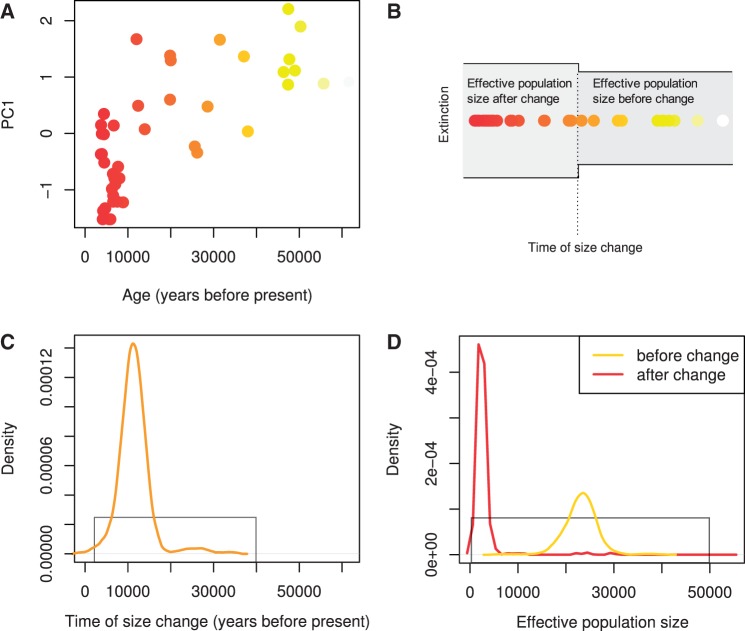
Verification
Claims the paper makes
The claims and statistics of this paper haven’t been checked yet.
Run the check — free, no account needed. It reads the open-access text and checks the sources it cites.
Claims other papers make about this one
Each is checked against this paper’s own text: does it say what the citing paper says it does?
The source backs part of the claim, not all of it — or backs it for a different population, condition or comparison.
In the citing paper
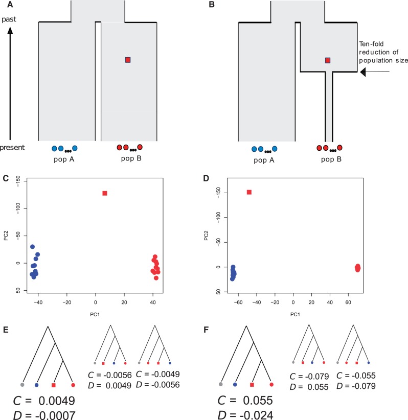
“It is notable that PCA clustering is sensitive to the sample size of different ancestries and also to their amount of genetic drift, which exaggerates principal component distances 207,208,211,212 .”
From Ancient DNA analysis (2021) · cites this paper as [212]
Experimental — accuracy not yet measured
Self-check
Percentages, sums and reported differences re-computed from the paper’s own numbers.
The self-check needs the paper’s full text.
Citations
Cites
Ancient Admixture in Human History
Patterson, N., Moorjani, P., Luo, Y., Mallick, S., Rohland, N., Zhan, Y., Genschoreck, T., Webster, T., & Reich, D. (2012) · Genetics · doi:10.1534/genetics.112.145037 · Cited by 2,848
Inference of population splits and mixtures from genome-wide allele frequency data
Pickrell, J. K., & Pritchard, J. K. (2012) · PLoS Genetics · doi:10.1371/journal.pgen.1002967 · Cited by 2,731
Inference of human population history from individual whole-genome sequences
Li, H., & Durbin, R. (2011) · Nature · doi:10.1038/nature10231 · Cited by 2,590
The complete genome sequence of a Neanderthal from the Altai Mountains
Prüfer, K., Racimo, F., Patterson, N., Jay, F., Sankararaman, S., Sawyer, S., Heinze, A., Renaud, G., Sudmant, P. H., de Filippo, C., et al. (2014) · Nature · doi:10.1038/nature12886 · Cited by 2,254
Genetic history of an archaic hominin group from Denisova Cave in Siberia
Reich, D., Green, R. E., Kircher, M., Krause, J., Patterson, N., Durand, E. Y., Viola, B., Briggs, A. W., Stenzel, U., Johnson, P. L. F., et al. (2010) · Nature · doi:10.1038/nature09710 · Cited by 1,991
A high-coverage genome sequence from an archaic denisovan individual
Meyer, M., Kircher, M., Gansauge, M.-T., Li, H., Racimo, F., Mallick, S., Schraiber, J. G., Jay, F., Prüfer, K., de Filippo, C., et al. (2012) · Science · doi:10.1126/science.1224344 · Cited by 1,967
Reconstructing Indian population history
Reich, D., Thangaraj, K., Patterson, N., Price, A. L., & Singh, L. (2009) · Nature · doi:10.1038/nature08365 · Cited by 1,674
Approximate Bayesian Computation (ABC) in practice
Csilléry, K., Blum, M. G. B., Gaggiotti, O. E., & François, O. (2010) · Trends in Ecology & Evolution · doi:10.1016/j.tree.2010.04.001 · Cited by 1,302
Upper Palaeolithic Siberian genome reveals dual ancestry of Native Americans
Raghavan, M., Skoglund, P., Graf, K. E., Metspalu, M., Albrechtsen, A., Moltke, I., Rasmussen, S., Stafford Jr, T. W., Orlando, L., Metspalu, E., et al. (2014) · Nature · doi:10.1038/nature12736 · Cited by 963
Self-citationAncient human genome sequence of an extinct Palaeo-Eskimo
Rasmussen, M., Li, Y., Lindgreen, S., Pedersen, J. S., Albrechtsen, A., Moltke, I., Metspalu, M., Metspalu, E., Kivisild, T., Gupta, R., et al. (2010) · Nature · doi:10.1038/nature08835 · Cited by 849
Recalibrating equus evolution using the genome sequence of an early middle pleistocene horse
Orlando, L., Ginolhac, A., Zhang, G., Froese, D., Albrechtsen, A., Stiller, M., Schubert, M., Cappellini, E., Petersen, B., Moltke, I., et al. (2013) · Nature · doi:10.1038/nature12323 · Cited by 841
A mitochondrial genome sequence of a hominin from Sima de los Huesos
Meyer, M., Fu, Q., Aximu-Petri, A., Glocke, I., Nickel, B., Arsuaga, J.-L., Martínez, I., Gracia, A., de Castro, J. M. B., Carbonell, E., et al. (2014) · Nature · doi:10.1038/nature12788 · Cited by 534
Separating endogenous ancient DNA from modern day contamination in a Siberian Neandertal
Skoglund, P., Northoff, B. H., Shunkov, M. V., Derevianko, A. P., Pääbo, S., Krause, J., & Jakobsson, M. (2014) · Proceedings of the National Academy of Sciences · doi:10.1073/pnas.1318934111 · Cited by 499
New insights into the Tyrolean Iceman's origin and phenotype as inferred by whole-genome sequencing
Keller, A., Graefen, A., Ball, M., Matzas, M., Boisguerin, V., Maixner, F., Leidinger, P., Backes, C., Khairat, R., Forster, M., et al. (2012) · Nature Communications · doi:10.1038/ncomms1701 · Cited by 437
Research works printed but not linked: 61
- Anderson, 2005, Serial SimCoal: a population genetics model for data from multiple populations and points in time, Bioinformatics, 21, 1733, 10.1093/bioinformatics/bti154 · DOI
- Anderson, 2000, Monte Carlo evaluation of the likelihood for N(e) from temporally spaced samples, Genetics, 156, 2109, 10.1093/genetics/156.4.2109 · DOI
- Beaumont, 2003, Estimation of population growth or decline in genetically monitored populations, Genetics, 164, 1139, 10.1093/genetics/164.3.1139 · DOI
- Beaumont, 2002, Approximate Bayesian computation in population genetics, Genetics, 162, 2025, 10.1093/genetics/162.4.2025 · DOI · Paper page
- Berthier, 2002, Likelihood-based estimation of the effective population size using temporal changes in allele frequencies: a genealogical approach, Genetics, 160, 741, 10.1093/genetics/160.2.741 · DOI
- Briggs, 2007, Patterns of damage in genomic DNA sequences from a Neandertal, Proc Natl Acad Sci U S A., 104, 14616, 10.1073/pnas.0704665104 · DOI · Paper page
- Briggs, 2010, Removal of deaminated cytosines and detection of in vivo methylation in ancient DNA, Nucleic Acids Res., 38, e87, 10.1093/nar/gkp1163 · DOI · Paper page
- Castroviejo-Fisher, 2011, Vanishing native American dog lineages, BMC Evol Biol., 11, 73, 10.1186/1471-2148-11-73 · DOI
- Chan, 2006, Bayesian estimation of the timing and severity of a population bottleneck from ancient DNA, PLoS Genet., 2, 451, 10.1371/journal.pgen.0020059 · DOI
- Chikhi, 2010, The confounding effects of population structure, genetic diversity and the sampling scheme on the detection and quantification of population size changes, Genetics, 186, 983, 10.1534/genetics.110.118661 · DOI
- DeGiorgio, 2013, Geographic sampling scheme as a determinant of the major axis of genetic variation in principal components analysis, Mol Biol Evol., 30, 480, 10.1093/molbev/mss233 · DOI
- Depaulis, 2009, Using classical population genetics tools with heterochroneous data: time matters!, PLoS One, 4, e5541, 10.1371/journal.pone.0005541 · DOI
- Drummond, 2007, BEAST: Bayesian evolutionary analysis by sampling trees, BMC Evol Biol., 7, 214, 10.1186/1471-2148-7-214 · DOI
- Drummond, 2005, Bayesian coalescent inference of past population dynamics from molecular sequences, Mol Biol Evol., 22, 1185, 10.1093/molbev/msi103 · DOI
- Durand, 2011, Testing for ancient admixture between closely related populations, Mol Biol Evol., 28, 2239, 10.1093/molbev/msr048 · DOI · Paper page
- Engelhardt, 2010, Analysis of population structure: a unifying framework and novel methods based on sparse factor analysis, PLoS Genet., 6, e1001117, 10.1371/journal.pgen.1001117 · DOI · Paper page
- Excoffier, 2011, Fastsimcoal: a continuous-time coalescent simulator of genomic diversity under arbitrarily complex evolutionary scenarios, Bioinformatics, 27, 1332, 10.1093/bioinformatics/btr124 · DOI
- Green, 2010, A draft sequence of the neandertal genome, Science, 328, 710, 10.1126/science.1188021 · DOI · Paper page
- Haak, 2005, Ancient DNA from the first European farmers in 7500-year-old Neolithic sites, Science, 310, 1016, 10.1126/science.1118725 · DOI
- Higuchi, 1984, DNA sequence from the quagga, an extinct member of the horse family, Nature, 312, 282, 10.1038/312282a0 · DOI
- Ho, 2011, Skyline-plot methods for estimating demographic history from nucleotide sequences, Mol Ecol Resour., 11, 423, 10.1111/j.1755-0998.2011.02988.x · DOI
- Hudson, 2002, Generating samples under a Wright–Fisher neutral model of genetic variation, Bioinformatics, 18, 337, 10.1093/bioinformatics/18.2.337 · DOI
- Jakobsson, 2009, COMPASS: a program for generating serial samples under an infinite sites model, Bioinformatics, 25, 2845, 10.1093/bioinformatics/btp534 · DOI
- Kaj, 2001, Coalescent theory for seed bank models, J Appl Probab., 38, 285, 10.1017/S0021900200019860 · DOI
- Kingman, 1982, The coalescent, Stochastic Process Appl., 13, 235, 10.1016/0304-4149(82)90011-4 · DOI
- Krause, 2010, A complete mtDNA genome of an early modern human from Kostenki, Russia, Curr Biol., 20, 231, 10.1016/j.cub.2009.11.068 · DOI · Paper page
- Krimbas, 1971, The genetics of Dacus oleae. V. Changes of esterase polymorphism in a natural population following insecticide control-selection or drift?, Evolution, 25, 454, 10.2307/2407343 · DOI
- McVean, 2009, A genealogical interpretation of principal components analysis, PLoS Genet., 5, e1000686, 10.1371/journal.pgen.1000686 · DOI · Paper page
- Mourier, 2012, Statistical guidelines for detecting past population shifts using ancient DNA, Mol Biol Evol., 29, 2241, 10.1093/molbev/mss094 · DOI
- Navascues, 2010, Combining contemporary and ancient DNA in population genetic and phylogeographical studies, Mol Ecol Resour., 10, 760, 10.1111/j.1755-0998.2010.02895.x · DOI
- Nei, 1973, Analysis of gene diversity in subdivided populations, Proc Natl Acad Sci U S A., 70, 3321, 10.1073/pnas.70.12.3321 · DOI · Paper page
- Nielsen, 2001, Distinguishing migration from isolation: a Markov chain Monte Carlo approach, Genetics, 158, 885, 10.1093/genetics/158.2.885 · DOI
- Nordborg, 1998, On the probability of Neanderthal ancestry, Am J Hum Genet., 63, 1237, 10.1086/302052 · DOI
- Novembre, 2008, Interpreting principal component analyses of spatial population genetic variation, Nat Genet., 40, 646, 10.1038/ng.139 · DOI
- Nyström, 2010, Temporal genetic change in the last remaining population of woolly mammoth, Proc R Soc B Biol Sci., 277, 2331, 10.1098/rspb.2010.0301 · DOI
- Nyström, 2012, Microsatellite genotyping reveals end-Pleistocene decline in mammoth autosomal genetic variation, Mol Ecol., 21, 3391, 10.1111/j.1365-294X.2012.05525.x · DOI
- Pääbo, 1985, Molecular cloning of ancient Egyptian mummy DNA, Nature, 314, 644, 10.1038/314644a0 · DOI
- Patterson, 2006, Population structure and eigenanalysis, PLoS Genet., 2, e190, 10.1371/journal.pgen.0020190 · DOI · Paper page
- Pritchard, 1999, Population growth of human Y chromosomes: a study of Y chromosome microsatellites, Mol Biol Evol., 16, 1791, 10.1093/oxfordjournals.molbev.a026091 · DOI
- Ramakrishnan, 2005, Detecting past population bottlenecks using temporal genetic data, Mol Ecol., 14, 2915, 10.1111/j.1365-294X.2005.02586.x · DOI
- Ramakrishnan, 2009, Using phylochronology to reveal cryptic population histories: review and synthesis of 29 ancient DNA studies, Mol Ecol., 18, 1310, 10.1111/j.1365-294X.2009.04092.x · DOI
- Rosenberg, 2005, Clines, clusters, and the effect of study design on the inference of human population structure, PLoS Genet., 1, e70, 10.1371/journal.pgen.0010070 · DOI
- Sánchez-Quinto, 2012, Genomic affinities of two 7,000-year-old Iberian hunter-gatherers, Curr Biol., 22, 1494, 10.1016/j.cub.2012.06.005 · DOI · Paper page
- Schlebusch, 2012, Genomic variation in seven Khoe-San groups reveals adaptation and complex African history, Science, 338, 374, 10.1126/science.1227721 · DOI
- Serre, 2004, No evidence of Neandertal mtDNA contribution to early modern humans, PLoS Biol., 2, e57, 10.1371/journal.pbio.0020057 · DOI
- Serre, 2004, Evidence for gradients of human genetic diversity within and among continents, Genome Res., 14, 1679, 10.1101/gr.2529604 · DOI · Paper page
- Shapiro, 2014, A Paleogenomic perspective on evolution and gene function: new insights from ancient DNA, Science, 343, 1236573, 10.1126/science.1236573 · DOI · Paper page
- Sheehan, 2013, Estimating variable effective population sizes from multiple genomes: a sequentially Markov conditional sampling distribution approach, Genetics, 194, 647, 10.1534/genetics.112.149096 · DOI
- Sjödin, 2014, Assessing the maximum contribution from ancient populations, Mol Biol Evol., 31, 1248, 10.1093/molbev/msu059 · DOI
- Skoglund, 2011, Estimation of population divergence times from non-overlapping genomic sequences: examples from dogs and wolves, Mol Biol Evol., 28, 1505, 10.1093/molbev/msq342 · DOI
- Skoglund, 2012, Origins and genetic legacy of Neolithic farmers and hunter–gatherers in Europe, Science, 336, 466, 10.1126/science.1216304 · DOI · Paper page
- Slatkin, 1991, Inbreeding coefficients and coalescence times, Genet Res., 58, 167, 10.1017/S0016672300029827 · DOI
- Tavare, 1997, Inferring coalescence times from DNA sequence data, Genetics, 145, 505, 10.1093/genetics/145.2.505 · DOI
- Vartanyan, 1993, Holocene dwarf mammoths from Wrangel Island in the Siberian Arctic, Nature, 362, 337, 10.1038/362337a0 · DOI
- Voight, 2005, Interrogating multiple aspects of variation in a full resequencing data set to infer human population size changes, Proc Natl Acad Sci U S A., 102, 18508, 10.1073/pnas.0507325102 · DOI · Paper page
- Wang, 2001, A pseudo-likelihood method for estimating effective population size from temporally spaced samples, Genet Res., 78, 243, 10.1017/S0016672301005286 · DOI
- Waples, 1989, Temporal variation in allele frequencies: testing the right hypothesis, Evolution, 43, 1236, 10.2307/2409359 · DOI
- Weir, 1996, Genetic data analysis II
- Wright, 1940, Breeding structure of populations in relation to speciation, Am Nat., 74, 232, 10.1086/280891 · DOI
- Wright, 1949, Population structure in evolution, Proc Am Philos Soc., 93, 471
- Wright, 1951, The genetical structure of populations, Ann Eugen., 15, 323, 10.1111/j.1469-1809.1949.tb02451.x · DOI
Cited by
Sorted by citations
Orlando, L., Allaby, R., Skoglund, P., Der Sarkissian, C., Stockhammer, P. W., Ávila-Arcos, M. C., Fu, Q., Krause, J., Willerslev, E., Stone, A. C., et al. (2021) · Nature Reviews Methods Primers · doi:10.1038/s43586-020-00011-0 · Cited by 411
Self-citation
Metadata
- Authors
- Skoglund, P., Sjödin, P., Skoglund, T., Lascoux, M., & Jakobsson, M.
- Venue
- Molecular Biology and Evolution
- Publisher
- Oxford University Press (OUP)
- Published
- 2014-06-17
- Volume
- 31
- Issue
- 9
- Pages
- 2516-2527
- ISSN
- 1537-1719
- 0737-4038
- PMC
- PMC4137715
- Cited by
- 60
- References
- 14
- Language
- en
About these checks
Registry, retraction, Cites and statistics results are computed, not judged, with one exception: a printed reference that no index lists is read once by a model before it counts as a citation error. Claims are extracted by a model and kept only when their quote appears verbatim in the text; each cited source is then checked, with a model’s help, for whether it says what the claim relies on. Those verdicts can be wrong — read the claim’s quote and the cited source before relying on one.
Statistics and arithmetic are recomputed, not judged.
Confidence bands are shown only for fields calibrated on our annotated test set. None is calibrated yet, so no band is shown.
What counts as a claim ›How we measure confidence ›How we check this ›
Are you an author, or do you see a problem with this page? Request a review
