

The DOI matches its Crossref record; 3 of the 3 references it cites were found in a registry or an index.
Canopy structure and topography jointly constrain the microclimate of human‐modified tropical landscapes
Abstract
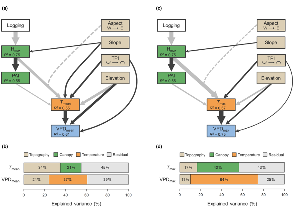
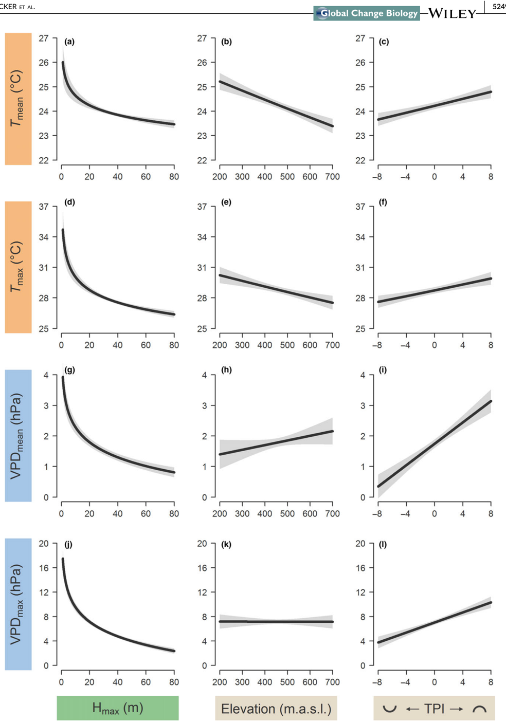
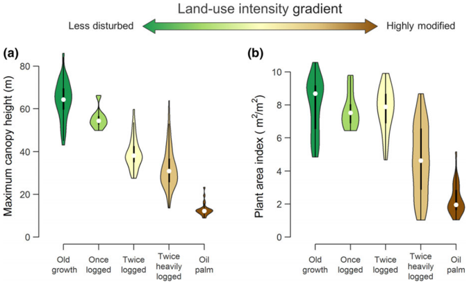
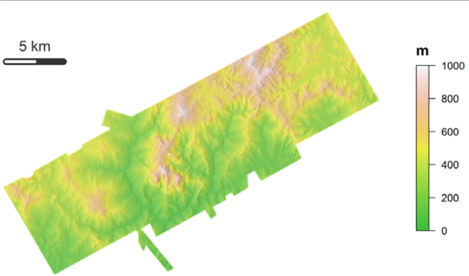
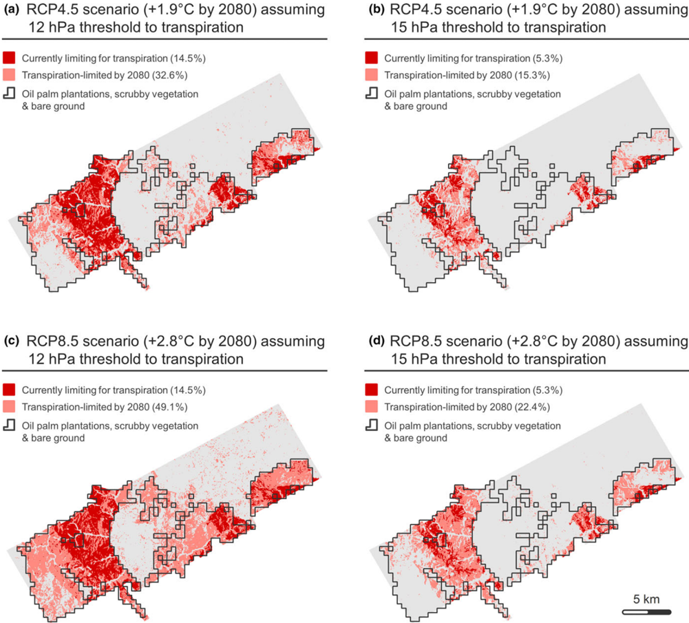
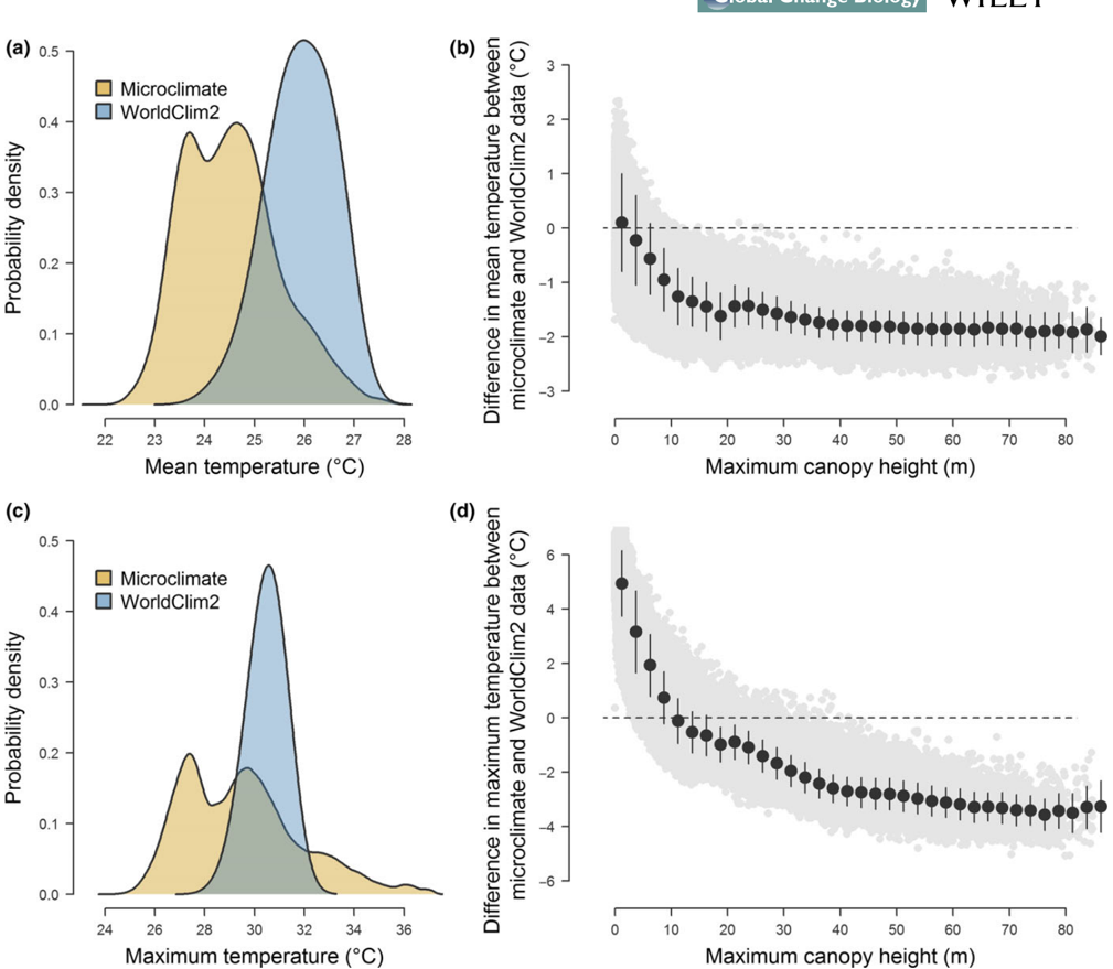
Local‐scale microclimatic conditions in forest understoreys play a key role in shaping the composition, diversity and function of these ecosystems. Consequently, understanding what drives variation in forest microclimate is critical to forecasting ecosystem responses to global change, particularly in the tropics where many species already operate close to their thermal limits and rapid land‐use transformation is profoundly altering local environments. Yet our ability to characterize forest microclimate at ecologically meaningful scales remains limited, as understorey conditions cannot be directly measured from outside the canopy. To address this challenge, we established a network of microclimate sensors across a land‐use intensity gradient spanning from old‐growth forests to oil‐palm plantations in Borneo. We then combined these observations with high‐resolution airborne laser scanning data to characterize how topography and canopy structure shape variation in microclimate both locally and across the landscape. In the processes, we generated high‐resolution microclimate surfaces spanning over 350 km 2 , which we used to explore the potential impacts of habitat degradation on forest regeneration under both current and future climate scenarios. We found that topography and vegetation structure were strong predictors of local microclimate, with elevation and terrain curvature primarily constraining daily mean temperatures and vapour pressure deficit (VPD), whereas canopy height had a clear dampening effect on microclimate extremes. This buffering effect was particularly pronounced on wind‐exposed slopes but tended to saturate once canopy height exceeded 20 m—suggesting that despite intensive logging, secondary forests remain largely thermally buffered. Nonetheless, at a landscape‐scale microclimate was highly heterogeneous, with maximum daily temperatures ranging between 24.2 and 37.2°C and VPD spanning two orders of magnitude. Based on this, we estimate that by the end of the century forest regeneration could be hampered in degraded secondary forests that characterize much of Borneo's lowlands if temperatures continue to rise following projected trends.
Overview
The claims and statistics of this paper haven’t been checked yet.
Run the check — free, no account needed. It reads the open-access text and checks the sources it cites.
Integrity signals
Registry
Cites
Statistics
Figures
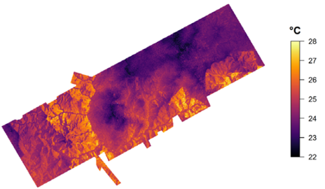
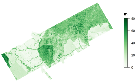
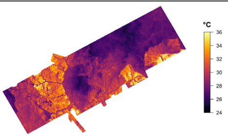
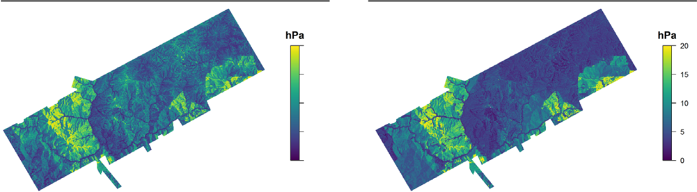
Verification
Claims the paper makes
The claims and statistics of this paper haven’t been checked yet.
Run the check — free, no account needed. It reads the open-access text and checks the sources it cites.
Claims other papers make about this one
Each is checked against this paper’s own text: does it say what the citing paper says it does?
In the citing paper
“While it has been shown that in the tropics, higher canopies provide a stronger dampening effect on microclimate extremes11”
From A high-resolution canopy height model of the Earth (2023) · cites this paper as [11]
Self-check
Percentages, sums and reported differences re-computed from the paper’s own numbers.
The self-check needs the paper’s full text.
Citations
Cites
Global analysis of thermal tolerance and latitude in ectotherms
Sunday, J. M., Bates, A. E., & Dulvy, N. K. (2011) · Proceedings of the Royal Society B: Biological Sciences · doi:10.1098/rspb.2010.1295 · Cited by 1,300
Biomass resilience of Neotropical secondary forests
Poorter, L., Bongers, F., Aide, T. M., Almeyda Zambrano, A. M., Balvanera, P., Becknell, J. M., Boukili, V., Brancalion, P. H. S., Broadbent, E. N., Chazdon, R. L., et al. (2016) · Nature · doi:10.1038/nature16512 · Cited by 1,210
García-Robledo, C., Kuprewicz, E. K., Staines, C. L., Erwin, T. L., & Kress, W. J. (2016) · Proceedings of the National Academy of Sciences · doi:10.1073/pnas.1507681113 · Cited by 306
Research works printed but not linked: 73
- 10.1016/j.jag.2017.10.009 · DOI
- 10.2307/1931468 · DOI
- 10.1175/1520-0493(1980)108<1046:TCOEPT>2.0.CO;2 · DOI
- 10.1002/ece3.3460 · DOI
- 10.1038/nclimate3071 · DOI
- 10.1016/bs.aecr.2017.12.005 · DOI
- 10.1371/journal.pone.0069679 · DOI
- 10.1017/S026646740000866X · DOI
- 10.1073/pnas.1605365113 · DOI
- 10.1111/j.1523-1739.2009.01338.x · DOI
- 10.2307/1313612 · DOI
- Clarke A., 2017, Principles of thermal ecology: Temperature, energy and life, pp.
- Coomes D. A., 2018, Airborne laser scanning of natural forests in New Zealand reveals the influences of wind on forest carbon, Forest Ecosystems, 5, 1, 10.1186/s40663-017-0119-6 · DOI
- 10.1073/pnas.1311190110 · DOI
- 10.1126/science.351.6270.234-a · DOI
- 10.1111/1365-2664.13023 · DOI
- 10.1371/journal.pone.0076296 · DOI
- 10.1111/j.1365-2486.2010.02263.x · DOI
- 10.1029/2007JG000632 · DOI
- 10.1038/s41467-017-02810-8 · DOI
- 10.1186/s12898-017-0141-0 · DOI
- 10.1371/journal.pone.0058093 · DOI
- 10.1038/ncomms7836 · DOI
- 10.1098/rstb.2011.0049 · DOI · Paper page
- 10.1371/journal.pone.0105541 · DOI
- 10.1002/joc.5086 · DOI · Paper page
- 10.1126/sciadv.1501392 · DOI
- 10.1038/srep32017 · DOI
- 10.1371/journal.pone.0101654 · DOI
- 10.1088/1748-9326/11/11/114022 · DOI
- 10.18637/jss.v017.i01 · DOI · Paper page
- Hardwick S. R., 2015, Interactions between vegetation and microclimate in a heterogeneous tropical landscape, Imperial College London, 138, pp
- 10.1016/j.agrformet.2014.11.010 · DOI
- Hijmans R. J., 2016, raster: Geographic data analysis and modeling. R package version, 2.5–8.
- 10.1111/j.1744-7429.1999.tb00135.x · DOI
- IPCC, 2014, IPCC, 2014: Climate Change 2014: Synthesis Report. Contribution of Working Groups I, II and III to the Fifth Assessment Report of the Intergovernmental Panel on Climate Change (eds Pachauri RK, Meyer LA), 151
- Jones C. D., 2003, Uncertainty in climate‐carbon‐cycle projections associated with the sensitivity of soil respiration to temperature, Tellus Series B, 55, 642
- 10.5194/bg-15-3811-2018 · DOI
- 10.1111/ele.12964 · DOI
- 10.1111/gcb.12750 · DOI
- 10.14358/PERS.80.9.863 · DOI · Paper page
- 10.1111/j.1365-2435.2008.01514.x · DOI
- 10.1016/j.agee.2015.01.027 · DOI
- 10.1111/2041-210X.12512 · DOI
- 10.1641/0006-3568(2002)052[0019:LRSFES]2.0.CO;2 · DOI
- 10.1111/ecog.02788 · DOI
- Lindeman R. H., 1980, Introduction to bivariate and multivariate analysis, 444
- 10.1098/rspb.2013.2236 · DOI
- 10.1088/1748-9326/aaa4ff · DOI · Paper page
- 10.1111/nph.15027 · DOI · Paper page
- 10.1029/2009JD013493 · DOI · Paper page
- 10.1093/treephys/25.10.1283 · DOI
- 10.1016/j.rse.2016.01.014 · DOI
- 10.1111/gcb.12257 · DOI
- R Core Development Team., 2016, R: A language and environment for statistical computing
- 10.1111/gcb.14068 · DOI
- 10.1111/gcb.13973 · DOI
- 10.1111/btp.12355 · DOI
- 10.1016/j.biocon.2015.02.018 · DOI
- 10.1111/gcb.13914 · DOI
- 10.1002/ece3.3262 · DOI
- 10.1016/j.foreco.2005.12.019 · DOI
- 10.2307/2259061 · DOI
- 10.1111/j.1461-0248.2012.01864.x · DOI
- 10.1002/ecs2.1797 · DOI
- 10.1088/1748-9326/aa6f97 · DOI
- 10.1038/ncomms15531 · DOI
- 10.1007/s13595-017-0628-z · DOI
- 10.1098/rstb.1999.0528 · DOI
- 10.1093/treephys/tpq015 · DOI
- 10.1111/1365-2435.12351 · DOI
- 10.1111/nph.12321 · DOI
- 10.1016/j.rse.2012.02.001 · DOI
Cited by
Sorted by citations
A high-resolution canopy height model of the Earth
Lang, N., Jetz, W., Schindler, K., & Wegner, J. D. (2023) · Nature Ecology & Evolution · doi:10.1038/s41559-023-02206-6 · Cited by 810
Soundscapes predict species occurrence in tropical forests
Sethi, S. S., Ewers, R. M., Jones, N. S., Sleutel, J., Shabrani, A., Zulkifli, N., & Picinali, L. (2022) · Oikos · doi:10.1111/oik.08525 · Cited by 34
Self-citation
Metadata
- Authors
- Jucker, T., Hardwick, S. R., Both, S., Elias, D. M. O., Ewers, R. M., Milodowski, D. T., Swinfield, T., & Coomes, D. A.
- Affiliations
- Forest Ecology and Conservation group, Department of Plant Sciences University of Cambridge Cambridge UK
- Blackett Laboratory, Department of Physics Imperial College London London UK
- School of Environmental and Rural Science University of New England Armidale NSW Australia
- Lancaster Environment Centre Lancaster University Lancaster UK
- Imperial College London Ascot UK
- School of GeoSciences University of Edinburgh Edinburgh UK
- Venue
- Global Change Biology
- Publisher
- Wiley
- Published
- 2018-09-23
- Volume
- 24
- Issue
- 11
- Pages
- 5243-5258
- ISSN
- 1354-1013
- 1365-2486
- Cited by
- 281
- References
- 3
- Language
- en
- Funders
- Natural Environment Research Council (NE/K016377/1)
About these checks
Registry, retraction, Cites and statistics results are computed, not judged, with one exception: a printed reference that no index lists is read once by a model before it counts as a citation error. Claims are extracted by a model and kept only when their quote appears verbatim in the text; each cited source is then checked, with a model’s help, for whether it says what the claim relies on. Those verdicts can be wrong — read the claim’s quote and the cited source before relying on one.
Statistics and arithmetic are recomputed, not judged.
Confidence bands are shown only for fields calibrated on our annotated test set. None is calibrated yet, so no band is shown.
What counts as a claim ›How we measure confidence ›How we check this ›
Are you an author, or do you see a problem with this page? Request a review
