

The DOI matches its Crossref record; 112 of the 113 references it cites were found in a registry or an index, and 1 are not checked yet.
The genetic and biochemical determinants of mRNA degradation rates in mammals
Open accessPublished version of a preprint
Abstract
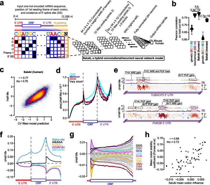
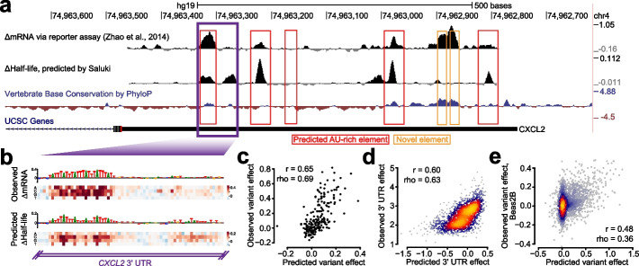
BACKGROUND: Degradation rate is a fundamental aspect of mRNA metabolism, and the factors governing it remain poorly characterized. Understanding the genetic and biochemical determinants of mRNA half-life would enable more precise identification of variants that perturb gene expression through post-transcriptional gene regulatory mechanisms. RESULTS: We establish a compendium of 39 human and 27 mouse transcriptome-wide mRNA decay rate datasets. A meta-analysis of these data identified a prevalence of technical noise and measurement bias, induced partially by the underlying experimental strategy. Correcting for these biases allowed us to derive more precise, consensus measurements of half-life which exhibit enhanced consistency between species. We trained substantially improved statistical models based upon genetic and biochemical features to better predict half-life and characterize the factors molding it. Our state-of-the-art model, Saluki, is a hybrid convolutional and recurrent deep neural network which relies only upon an mRNA sequence annotated with coding frame and splice sites to predict half-life (r=0.77). The key novel principle learned by Saluki is that the spatial positioning of splice sites, codons, and RNA-binding motifs within an mRNA is strongly associated with mRNA half-life. Saluki predicts the impact of RNA sequences and genetic mutations therein on mRNA stability, in agreement with functional measurements derived from massively parallel reporter assays. CONCLUSIONS: Our work produces a more robust ground truth for transcriptome-wide mRNA half-lives in mammalian cells. Using these revised measurements, we trained Saluki, a model that is over 50% more accurate in predicting half-life from sequence than existing models. Saluki succinctly captures many of the known determinants of mRNA half-life and can be rapidly deployed to predict the functional consequences of arbitrary mutations in the transcriptome.
Overview
The claims and statistics of this paper haven’t been checked yet.
Run the check — free, no account needed. It reads the open-access text and checks the sources it cites.
Integrity signals
Registry
Cites
Statistics
Figures
Verification
Claims the paper makes
The claims and statistics of this paper haven’t been checked yet.
Run the check — free, no account needed. It reads the open-access text and checks the sources it cites.
Claims other papers make about this one
Each is checked against this paper’s own text: does it say what the citing paper says it does?
The source backs part of the claim, not all of it — or backs it for a different population, condition or comparison.
In the citing paper
“Similarly, sequence-based models of post-transcriptional regulation rely on genome annotations and transformed measurements extracted from RNA-seq to isolate each regulatory mechanism (for example, percent spliced-in for splicing)14–23.”
From Predicting RNA-seq coverage from DNA sequence as a unifying model of gene regulation (2025) · cites this paper as [23]
Experimental — accuracy not yet measuredThe source backs part of the claim, not all of it — or backs it for a different population, condition or comparison.
In the citing paper
“Furthermore, we did not find sequence elements related to mRNA half-life in Borzoi’s sequence attributions23,82.”
From Predicting RNA-seq coverage from DNA sequence as a unifying model of gene regulation (2025) · cites this paper as [23]
Experimental — accuracy not yet measuredThe cited source says what the claim attributes to it.
In the citing paper
“Prior work has demonstrated strong relationships between codon usage and mRNA half-life23,78.”
From Predicting RNA-seq coverage from DNA sequence as a unifying model of gene regulation (2025) · cites this paper as [23]
The check wasn’t confident either way, so it gives no verdict — never disputed.
In the citing paper
“Borzoi performs better at longer distances (dAUPRC > 0.050 at 2,000 bp) with a more comparable performance closer to the PAS (dAUPRC = 0.025 at 50 bp) (Fig. 6g).”
From Predicting RNA-seq coverage from DNA sequence as a unifying model of gene regulation (2025) · cites this paper as [23]
Experimental — accuracy not yet measured
Self-check
Percentages, sums and reported differences re-computed from the paper’s own numbers.
The self-check needs the paper’s full text.
Citations
Cites
BEDTools: a flexible suite of utilities for comparing genomic features
Quinlan, A. R., & Hall, I. M. (2010) · Bioinformatics · doi:10.1093/bioinformatics/btq033 · Cited by 27,437
Most mammalian mRNAs are conserved targets of microRNAs
Friedman, R. C., Farh, K. K.-H., Burge, C. B., & Bartel, D. P. (2009) · Genome Research · doi:10.1101/gr.082701.108 · Cited by 8,462
Predicting effective microRNA target sites in mammalian mRNAs
Agarwal, V., Bell, G. W., Nam, J.-W., & Bartel, D. P. (2015) · eLife · doi:10.7554/elife.05005 · Cited by 7,318
Self-citationGlobal quantification of mammalian gene expression control
Schwanhäusser, B., Busse, D., Li, N., Dittmar, G., Schuchhardt, J., Wolf, J., Chen, W., & Selbach, M. (2011) · Nature · doi:10.1038/nature10098 · Cited by 6,566 · cited 1×
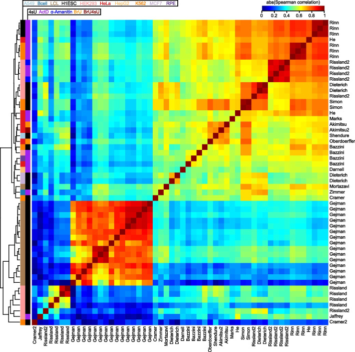
“GroupID Method Species Cell types Samples Reference Akimitsu BrU (BRIC-seq) H HeLa 1 [45] Akimitsu2 BrU+4sU (Dyrec-seq) H HeLa 1 [46] Bazzini 4sU (SLAM-seq), ActD H K562, RPE, HeLa, HEK293 4 [29] Cramer 4sU (TT-seq) H K562 1 [47] Cramer2 4sU (TT-seq) H K562 1 [43] Darnell ActD H HepG2 1 [38] Dieterich 4sU H HEK293, MC…”
The GTEx Consortium atlas of genetic regulatory effects across human tissues
The GTEx Consortium, Aguet, F., Anand, S., Ardlie, K. G., Gabriel, S., Getz, G. A., Graubert, A., Hadley, K., Handsaker, R. E., Huang, K. H., et al. (2020) · Science · doi:10.1126/science.aaz1776 · Cited by 5,547
Li, J.-H., Liu, S., Zhou, H., Qu, L.-H., & Yang, J.-H. (2014) · Nucleic Acids Research · doi:10.1093/nar/gkt1248 · Cited by 4,686
N6-methyladenosine-dependent regulation of messenger RNA stability
Wang, X., Lu, Z., Gomez, A., Hon, G. C., Yue, Y., Han, D., Fu, Y., Parisien, M., Dai, Q., Jia, G., et al. (2014) · Nature · doi:10.1038/nature12730 · Cited by 4,558
MicroRNA Targeting Specificity in Mammals: Determinants beyond Seed Pairing
Grimson, A., Farh, K. K.-H., Johnston, W. K., Garrett-Engele, P., Lim, L. P., & Bartel, D. P. (2007) · Molecular Cell · doi:10.1016/j.molcel.2007.06.017 · Cited by 3,766
Bartel, D. P. (2018) · Cell · doi:10.1016/j.cell.2018.03.006 · Cited by 3,751
CADD: predicting the deleteriousness of variants throughout the human genome
Rentzsch, P., Witten, D., Cooper, G. M., Shendure, J., & Kircher, M. (2019) · Nucleic Acids Research · doi:10.1093/nar/gky1016 · Cited by 3,534
Research works printed but not linked: 3
- [cited 2022 Feb 22]. Available from: https://academic.oup.com/g3journal/article-abstract/12/1/jkab404/6446033.
- Ba JL, Kiros JR, Hinton GE. Layer normalization. arXiv preprint arXiv:160706450. arxiv.org; 2016; Available from: http://arxiv.org/abs/1607.06450 · arXiv
- Chung J, Gulcehre C, Cho K, Bengio Y. Empirical evaluation of gated recurrent neural networks on sequence modeling. arXiv [cs.NE]. 2014. Available from: http://arxiv.org/abs/1412.3555 · arXiv
Cited by
Sorted by citations
Items 101–154 of 154
Martinez, M. B., Williamson, C. J., Cazares, T. A., Tang, C., Debets, M. F., & Gangras, P. (2025) · Nucleic Acid Therapeutics · doi:10.1177/21593337251377561 · Cited by 1
Wang, Y., Cai, Y., Wu, Z., Zhang, J., Turtle, L. C. W., & Meng, J. (2026) · Bioinformatics and Biology Insights · doi:10.1177/11779322261431255 · Cited by 1
Deep learning model for predicting mRNA half-life based on 3′UTR sequences
Jin, X., Wang, W., Wang, A., Zhang, Y., Mao, Y., & Zhang, D. (2026) · Biochemical and Biophysical Research Communications · doi:10.1016/j.bbrc.2026.153691 · Cited by 1
Decoding the language of messenger RNA
Wang, J., Zheng, D., & Agarwal, V. (2026) · Nature Methods · doi:10.1038/s41592-026-03032-x · Cited by 1
Self-citationFrom mutation to degradation: predicting nonsense-mediated mRNA decay with NMDap
Saadat, A., & Fellay, J. (2026) · Biochemical and Biophysical Research Communications · doi:10.1016/j.bbrc.2026.153833 · Cited by 1
Crowdsourcing to predict RNA degradation and secondary structure
Hendrix, D. A. (2023) · Nature Machine Intelligence · doi:10.1038/s42256-023-00615-7 · Cited by 1
Splice_sim: a nucleotide conversion-enabled RNA-seq simulation and evaluation framework
Popitsch, N. P., Neumann, T., von Haeseler, A., & Ameres, S. L. (2024) · Genome biology · doi:10.1186/s13059-024-03313-8 · Cited by 1
Karner, H. M., Mittmann, T., Chen, V., Borah, A. A., Langen, A., Yousefi, H., Fish, L., Zaro, B. W., Navickas, A., & Goodarzi, H. (2026) · Science Advances · doi:10.1126/sciadv.aea9061 · Cited by 1
Deciphering the Impact of Genetic Variation on Human PolyadenylationPreprint
Linder, J., Kundaje, A. B., & Seelig, G. (2022) · bioRxiv (Cold Spring Harbor Laboratory) · doi:10.1101/2022.05.09.491198 · Cited by 1
Predicting cell population-specific gene expression from genomic sequencePreprint
Michielsen, L., Reinders, M. J. T., & Mahfouz, A. E. (2022) · bioRxiv (Cold Spring Harbor Laboratory) · doi:10.1101/2022.09.06.506837 · Cited by 1
Sasse, A., Chikina, M. D., & Mostafavi, S. (2023) · bioRxiv (Cold Spring Harbor Laboratory) · doi:10.1101/2023.11.10.566588 · Cited by 1
Su, J.-Y., Wang, Y.-L., Hsieh, Y.-T., Chang, Y.-C., Yang, C., Kang, Y., Huang, Y., & Lin, C. (2024) · eLife · doi:10.7554/elife.97682.1 · Cited by 1
Su, J.-Y., Wang, Y.-L., Hsieh, Y.-T., Chang, Y.-C., Yang, C., Kang, Y., Huang, Y., & Lin, C. (2025) · eLife · doi:10.7554/elife.97682.2 · Cited by 1
A systematic delineation of 3′UTR regulatory elements and their contextual associations
Liang, N., Li, J., Ding, Y., Wang, Y., Champer, J., Ren, L., & Gao, G. (2026) · Cell Systems · doi:10.1101/2025.06.09.658412 · Cited by 1
Global inhibition of deadenylation stabilizes the transcriptome in mitotic cellsPreprint
Khalizeva, E., Latifkar, A., Bartel, D. P., Ly, J., & Cheeseman, I. M. (2025) · bioRxiv (Cold Spring Harbor Laboratory) · doi:10.1101/2025.07.22.666109 · Cited by 1
Chao, K.-H., Mao, A., Liu, A., Salzberg, S. L., & Pertea, M. (2025) · eLife · doi:10.7554/elife.107454.1 · Cited by 1
Neuronal activity triggers widespread changes in RNA stabilityPreprint
Duffy, E. E., Patop, I. L., Kalaora, S., Assad, E. G., Koren, S. A., Traunmüller, L., Krüttner, S., Pajarillo, N. S., Finander, B., Barsdale, Z., et al. (2025) · bioRxiv (Cold Spring Harbor Laboratory) · doi:10.1101/2025.09.05.674581 · Cited by 1
RNA degradation modulates unique aging-related gene expression in naked mole-ratsPreprint
Matsubara, R., Wu, J., Ozeki, A. N., Kawamura, Y., Hamada, M., Miura, K., & Akimitsu, N. (2025) · bioRxiv (Cold Spring Harbor Laboratory) · doi:10.1101/2025.11.28.691058 · Cited by 1
Enigma: An Efficient Model for Deciphering Regulatory GenomicsPreprint
Jung, A., Zhu, H., Li, R., Gao, A. J., Lau, T., Chu, V. S., Lim, D., Cole, C. B., Lee, L. J., Celaj, A., et al. (2025) · bioRxiv (Cold Spring Harbor Laboratory) · doi:10.64898/2025.12.18.694875 · Cited by 2
Anti‐SARS‐CoV ‐2 mRNA vaccines, their efficiency, side effects and controversies
Kuśnierczyk, P. (2023) · Scandinavian Journal of Immunology · doi:10.1111/sji.13310 · Cited by 2
Михайловна, М. А., & Pashenkov, M. V. (2023) · Immunologiya · doi:10.33029/1816-2134-2023-44-5-534-544
Gameiro, P. A., Foskolou, I. P., Martens, A., Kuret, K., Mozos, I. R. D. L., Hozjan, Ž., Kot, V., Faraway, R., Vermeulen, M., Wolkers, M. C., et al. (2024) · Research Square · doi:10.21203/rs.3.rs-4768725/v1
Passive shaping of intra- and intercellular m6A dynamics via mRNA metabolismPreprint
Dierks, D., Shachar, R., Nir, R., García-Campos, M. A., Uzonyi, A., Toth, U., Rossmanith, W., Lasman, L., Slobodin, B., Hanna, J. H., et al. (2024) · eLife · doi:10.7554/elife.100448.1
Cell-type specific prediction of RNA stability from RNA-protein interactionsPreprint
Saran, S., Lebedeva, S., Hirsekorn, A., & Ohler, U. (2024) · bioRxiv (Cold Spring Harbor Laboratory) · doi:10.1101/2024.11.19.624283
Pol II degradation activates cell death independently from the loss of transcriptionPreprint
Harper, N. W., Birdsall, G. A., Honeywell, M. E., Pai, A. A., & Lee, M. J. (2024) · bioRxiv (Cold Spring Harbor Laboratory) · doi:10.1101/2024.12.09.627542
Hidding, I. J., Vila, A. V., Hu, S., Bourgonje, A. R., van Gijn, M. E., Maassen, W. T. K., van der Vries, G. B., Ruigrok, R. A. A. A., Andreu‐Sánchez, S., Jansen, B. H., et al. (2024) · medRxiv · doi:10.1101/2024.12.09.24318484
Passive shaping of intra- and intercellular m6A dynamics via mRNA metabolismPreprint
Dierks, D., Shachar, R., Nir, R., García-Campos, M. A., Uzonyi, A., Wiener, D., Toth, U., Rossmanith, W., Lasman, L., Slobodin, B., et al. (2025) · eLife · doi:10.7554/elife.100448.2
Ebbert, M., Ho, A., Page, M. L., Dutch, B., Byer, B. K., Hankins, K. L., Sabra, H. W., Heberle, B. A., Wadsworth, M. E., Fox, G. A., et al. (2026) · Nucleic Acids Research · doi:10.1093/nar/gkag704
Wang, L., Zhou, Y., Yu, Z., Wu, P., Lu, Z., & Ma, L. (2025) · Cell Reports Methods · doi:10.1016/j.crmeth.2025.101087
Chao, K.-H., Mao, A., Liu, A., Salzberg, S. L., & Pertea, M. (2025) · eLife · doi:10.7554/elife.107454.2 · Cited by 1
Neighboring codon adjacent nucleotides have a conserved influence on mRNA decayPreprint
Sorenson, R. S., & Sieburth, L. (2025) · bioRxiv (Cold Spring Harbor Laboratory) · doi:10.1101/2025.11.17.688958
Felce, C., Schraiber, J. G., Krishnaswamy, M., Cope, A. L., Pachter, L. S., & Pennell, M. W. (2025) · bioRxiv (Cold Spring Harbor Laboratory) · doi:10.1101/2025.11.24.690267
Decoding UTRs by applying explainable AI to a genomic foundation modelPreprint
Brase, L., Creamer, D. R., Shapovalova, Y., Ashe, M., Ashe, H. L., & Rattray, M. (2025) · bioRxiv (Cold Spring Harbor Laboratory) · doi:10.64898/2025.12.04.692303
Integrated analysis of post-transcriptional regulations reveals insights into acute myeloid leukemia
Khadra, E., Iqbal, Z., Gall, M. L., Clary, G., Levavasseur, F., Tuerdi, Z., Dussiau, C., Rombaut, D., Templé, M., Friedrich, C., et al. (2025) · Communications Biology · doi:10.1038/s42003-025-09156-8
Kishimoto, T., Nishimura, K., Morishita, K., Fukuda, A., Miyamae, Y., Kumagai, Y., Sumaru, K., Nakanishi, M., Hisatake, K., & Sano, M. (2024) · Figshare · doi:10.6084/m9.figshare.25010399
Qiu, Q., Zhang, H., Xia, Z., Gao, W. N. D., Leu, J., Liang, D., Li, Y., Su, Y., Feierman, E. R., Horn, V., et al. (2026) · bioRxiv (Cold Spring Harbor Laboratory) · doi:10.64898/2026.01.29.702431
CRISPR mutagenesis of the MYC locus reveals a druggable ultraconserved RNA element
Shi, P., Yang, F., Tala, F. N. U., Huang, W., Xing, L., Alam, S., Dai, W., Aparicio, A. O., Kalicki, C. H., Trehan, A., et al. (2026) · Cell · doi:10.64898/2026.01.29.702547
Michielsen, L., Hsu, J., Joglekar, A., Belchikov, N., Reinders, M. J. T., Tilgner, H., & Mahfouz, A. E. (2026) · Genome biology · doi:10.1186/s13059-026-04015-z · Cited by 3
Benchmarking tissue- and cell type-of-origin deconvolution in cell-free transcriptomicsPreprint
Ioannou, A., Friman, E. T., Daub, C. O., Bickmore, W. A., & Biddie, S. C. (2026) · bioRxiv (Cold Spring Harbor Laboratory) · doi:10.64898/2026.03.05.709833
Mueller, L., Glaß, M., Preckwinkel, P., Hüttelmaier, S., Haemmerle, M., & Gutschner, T. (2026) · bioRxiv (Cold Spring Harbor Laboratory) · doi:10.64898/2026.04.24.720399
Fine-scale structural information substantially improves mRNA therapeutic stability prediction
Yi, S., Ali, S. E., Jadeja, Y., Davis, J. W., & Metkar, M. (2026) · Molecular Therapy — Nucleic Acids · doi:10.1016/j.omtn.2026.102960 · Cited by 1
Modeling the Language of Codons with Artificial Intelligence
Lemay-St-Denis, C., & Kolodny, R. (2026) · Annual Review of Biomedical Data Science · doi:10.1146/annurev-biodatasci-092624-105741
Transcripts enriched in codons that trigger P‐site tRNA ‐mediated mRNA decay possess stable mRNA
Carneiro, R. L., & Palhano, F. L. (2026) · FEBS Open Bio · doi:10.1002/2211-5463.70277
Wang, S., & Zhang, C. H. I. (2026) · bioRxiv (Cold Spring Harbor Laboratory) · doi:10.64898/2026.06.19.733389
Unveiling the Hidden Rules: Enhancing NMD Prediction for Protein-Truncating VariantsPreprint
Egab, I., Schmidt, J., Cortázar, M. A., Xu, J., Orchard, P., Dawood, M., Bozkurt‐Yozgatli, T., Koh, J., Mestroni, L., Taylor, M., et al. (2026) · bioRxiv (Cold Spring Harbor Laboratory) · doi:10.64898/2026.06.26.734884
Farghadan, A., Schmitz, R. J., Jackson, S. A., & Pickering, E. M. (2026) · bioRxiv (Cold Spring Harbor Laboratory) · doi:10.64898/2026.07.16.738979
Application of Machine Learning in mRNA Therapeutics Development
Liu, C. X., Ouyang, L., Xu, H., Liu, S., & Ma, B. (2026) · Pharmaceutical Fronts · doi:10.1055/a-2899-0538
Dao, W., Zhang, S., Zhang, T., Fan, X., & Miao, Y. (2026) · Animals · doi:10.3390/ani16172700
Spatial mapping of RNA turnover kinetics in the mouse brain
Qiu, Q., Zhang, H., Xia, Z., Gao, W., Leu, J. I., Liang, D., Li, Y., Fan, L., Su, Y., Feierman, E. R., et al. (2026) · Nature Neuroscience · doi:10.1038/s41593-026-02420-y
Extending the reach of transcription factors to mRNA stability
Galvan, B., Ongena, L., Claes, M., Mariavelle, E., & Dequiedt, F. (2026) · Trends Open · doi:10.1016/j.treopn.2026.07.017
Sequence optimization targeting mRNA stability enhances monoclonal antibody titers in CHO cells
Schneckener, S., Haag, K., Leweke, S., Wolf, T., & Mayer‐Bartschmid, A. (2026) · New Biotechnology · doi:10.1016/j.nbt.2026.09.004
Short-lived lncRNAs as candidate kinetic sensors of cellular stress
Tani, H. (2026) · Biochimica et Biophysica Acta (BBA) - Gene Regulatory Mechanisms · doi:10.1016/j.bbagrm.2026.195184
ContiTE: continuous manifold MoE for few-shot cross-tissue mRNA translation efficiency prediction
Wei, Y., Zhang, Q., Huo, S., & Zhou, X. (2026) · Briefings in Bioinformatics · doi:10.1093/bib/bbag518
Karimzadeh, M., Fish, L., Karner, H. M., Linder, J., Emadi, A., Hernández-Corchado, A., Smaili, F. Z., Ghavami, K., Stewart, E. S., Wang, B., et al. (2026) · bioRxiv (Cold Spring Harbor Laboratory) · doi:10.64898/2026.10.12.758580
Self-citation
Metadata
- Authors
- Agarwal, V., & Kelley, D. R.
- Affiliations
- Calico Life Sciences (US)
- Corresponding author
- Agarwal, Vikram
- Kelley, David R.
- Venue
- Genome Biology
- Published
- 2022-11-23
- Volume
- 23
- Issue
- 1
- Pages
- 245-245
- ISSN
- 1465-6906 (ISSN-L)
- 1474-760X
- PMC
- PMC9684954
- OpenAlex
- W4309925698
- Cited by
- 155
- References
- 111
- Citations by year
- 2026: 38 · 2025: 57 · 2024: 36 · 2023: 18 · 2022: 5
- FWCI
- 3.02
- Type
- journal article
- Language
- en
- Open access
- gold
- doi.org
- Locations
- Genome biology (publishedVersion, cc-by)
- bioRxiv (Cold Spring Harbor Laboratory) (acceptedVersion, cc-by-nc-nd)
- PubMed Central (publishedVersion, cc-by)
- PubMed (publishedVersion)
- DOAJ (DOAJ: Directory of Open Access Journals) (submittedVersion, cc-by-sa)
- Funders
- Calico Life Sciences LLC
- Topics
- Life Sciences › Biochemistry, Genetics and Molecular Biology › Molecular Biology › RNA Research and Splicing
- Life Sciences › Biochemistry, Genetics and Molecular Biology › Molecular Biology › RNA and protein synthesis mechanisms
- Life Sciences › Biochemistry, Genetics and Molecular Biology › Molecular Biology › RNA regulation and disease
- Keywords
- mRNA half-life, mRNA degradation rate, mRNA stability, post-transcriptional regulation, deep neural network inference, splice sites, RNA-binding motif, codon position, measurement bias correction, massively parallel reporter assay
- MeSH terms
- Animals, Biological Assay, Humans, Mammals, RNA, Messenger, RNA Stability, Mice, Transcriptome
About these checks
Registry, retraction, Cites and statistics results are computed, not judged, with one exception: a printed reference that no index lists is read once by a model before it counts as a citation error. Claims are extracted by a model and kept only when their quote appears verbatim in the text; each cited source is then checked, with a model’s help, for whether it says what the claim relies on. Those verdicts can be wrong — read the claim’s quote and the cited source before relying on one.
Statistics and arithmetic are recomputed, not judged.
Confidence bands are shown only for fields calibrated on our annotated test set. None is calibrated yet, so no band is shown.
What counts as a claim ›How we measure confidence ›How we check this ›
Are you an author, or do you see a problem with this page? Request a review
