CoChat

Efficient Reverse-Engineering of a Developmental Gene Regulatory Network

Open access

The DOI matches its Crossref record; 111 of the 113 references it cites were found in a registry or an index.

Abstract

Understanding the complex regulatory networks underlying development and evolution of multi-cellular organisms is a major problem in biology. Computational models can be used as tools to extract the regulatory structure and dynamics of such networks from gene expression data. This approach is called reverse engineering. It has been successfully applied to many gene networks in various biological systems. However, to reconstitute the structure and non-linear dynamics of a developmental gene network in its spatial context remains a considerable challenge. Here, we address this challenge using a case study: the gap gene network involved in segment determination during early development of Drosophila melanogaster. A major problem for reverse-engineering pattern-forming networks is the significant amount of time and effort required to acquire and quantify spatial gene expression data. We have developed a simplified data processing pipeline that considerably increases the throughput of the method, but results in data of reduced accuracy compared to those previously used for gap gene network inference. We demonstrate that we can infer the correct network structure using our reduced data set, and investigate minimal data requirements for successful reverse engineering. Our results show that timing and position of expression domain boundaries are the crucial features for determining regulatory network structure from data, while it is less important to precisely measure expression levels. Based on this, we define minimal data requirements for gap gene network inference. Our results demonstrate the feasibility of reverse-engineering with much reduced experimental effort. This enables more widespread use of the method in different developmental contexts and organisms. Such systematic application of data-driven models to real-world networks has enormous potential. Only the quantitative investigation of a large number of developmental gene regulatory networks will allow us to discover whether there are rules or regularities governing development and evolution of complex multi-cellular organisms.

Overview

The claims and statistics of this paper haven’t been checked yet.

Free: it reads the open-access text and checks the first 5 claims that cite a source we can check. Create a free account to check every claim.

A few free checks a day · papers already verified open instantly · results are public

Integrity signals

Registry

Crossref · 10.1371/journal.pcbi.1002589

Cites

111 of 111 references verified0 citation errors · 0 not checkable

Statistics

Figures

Figure 1 The gene circuit method. Top panel: a Drosophila embryo is modelled as a row of nuclei that undergo mitosis. Each nucleus contains four gap genes: hunchback (hb), Krüppel (Kr), giant (gt) and knirps (kni). The products of these genes diffuse, decay, and interact with each other to regulate gene expression. In addition gap genes are regulated by four external inputs, provided by the gene products of bicoid (bcd), caudal (cad), tailless (tll) and huckebein (hkb). Central circle: fitting the model to quantitative, spatial expression data is done via an iterative optimisation algorithm. A gene circuit with random regulatory parameters is used as the starting point for an exploration of parameter space. This is achieved by repeatedly changing parameter values to yield new gene circuit solutions. For each of these solutions model output is calculated and compared to the data by evaluating the sum of squared differences between the two. New gene circuit solutions are selected according to a global optimisation strategy (see Materials and Methods). The aim is to improve the fit to the gene expression data over many iterations until no further improvement can be achieved. Bottom panel: gene circuits that accurately reproduce expression data contain parameter estimates that encode a specific regulatory network structure. These models are analysed to yield insights into the regulatory dynamics and function of each interaction in the network.
Figure 1 The gene circuit method. Top panel: a Drosophila embryo is modelled as a row of nuclei that undergo mitosis. Each nucleus contains four gap genes: hunchback (hb), Krüppel (Kr), giant (gt) and knirps (kni). The products of these genes diffuse, decay, and interact with each other to regulate gene expression. In addition gap genes are regulated by four external inputs, provided by the gene products of bicoid (bcd), caudal (cad), tailless (tll) and huckebein (hkb). Central circle: fitting the model to quantitative, spatial expression data is done via an iterative optimisation algorithm. A gene circuit with random regulatory parameters is used as the starting point for an exploration of parameter space. This is achieved by repeatedly changing parameter values to yield new gene circuit solutions. For each of these solutions model output is calculated and compared to the data by evaluating the sum of squared differences between the two. New gene circuit solutions are selected according to a global optimisation strategy (see Materials and Methods). The aim is to improve the fit to the gene expression data over many iterations until no further improvement can be achieved. Bottom panel: gene circuits that accurately reproduce expression data contain parameter estimates that encode a specific regulatory network structure. These models are analysed to yield insights into the regulatory dynamics and function of each interaction in the network.CC BY · PubMed Central
Figure 2 Image acquisition and processing. As an example we show quantification of kni expression. (A–D) Embryo images are acquired using wide-field microscopy: unprocessed bright-field (A), DAPI counter-stain (B), and DIC images (C), as well as higher-resolution details of membrane morphology using DIC (D). Whole-embryo DIC images (as shown in C) are subjected to a sequence of image segmentation steps: 1. convert the image to gray-scale, 2. adjust gamma, 3. invert image, 4. apply Sobel edge detection (E), followed by 5. dilation operations, 6. filling of holes, and 7. removal of blobs touching the image border. Only the largest blob is kept, and Gaussian smoothing is applied to generate a binary mask covering the embryo (F). Whole-embryo masks are used to crop bright field (A), DAPI (B) and DIC (C) images, which are then rotated and flipped to orient them anterior to the left and dorsal to the top (G–J). The midline of the embryo is identified by using the skeleton of the whole-embryo mask, which is then approximated by a spline curve for smoothing and pruning of superfluous skeleton branches (K). We establish a band of 10% mask height along the midline of the embryo (K), which is overlain on the bright-field image (H) as shown in (L). A raw expression profile is extracted from this band (M), which shows high and irregular non-specific background. To eliminate this background, profiles are manually annotated and expression boundaries are approximated by cubic spline curves (M). We calculate the median position of extracted boundary positions for each expression profile per time stage and normalise the data (N: boundaries from individual embryos in black, median boundary in red). Median boundaries from multiple time classes are integrated to create an expression profile along the A–P axis though developmental time (O: contour plot with interpolated data between time classes). See main text for details.
Figure 2 Image acquisition and processing. As an example we show quantification of kni expression. (A–D) Embryo images are acquired using wide-field microscopy: unprocessed bright-field (A), DAPI counter-stain (B), and DIC images (C), as well as higher-resolution details of membrane morphology using DIC (D). Whole-embryo DIC images (as shown in C) are subjected to a sequence of image segmentation steps: 1. convert the image to gray-scale, 2. adjust gamma, 3. invert image, 4. apply Sobel edge detection (E), followed by 5. dilation operations, 6. filling of holes, and 7. removal of blobs touching the image border. Only the largest blob is kept, and Gaussian smoothing is applied to generate a binary mask covering the embryo (F). Whole-embryo masks are used to crop bright field (A), DAPI (B) and DIC (C) images, which are then rotated and flipped to orient them anterior to the left and dorsal to the top (G–J). The midline of the embryo is identified by using the skeleton of the whole-embryo mask, which is then approximated by a spline curve for smoothing and pruning of superfluous skeleton branches (K). We establish a band of 10% mask height along the midline of the embryo (K), which is overlain on the bright-field image (H) as shown in (L). A raw expression profile is extracted from this band (M), which shows high and irregular non-specific background. To eliminate this background, profiles are manually annotated and expression boundaries are approximated by cubic spline curves (M). We calculate the median position of extracted boundary positions for each expression profile per time stage and normalise the data (N: boundaries from individual embryos in black, median boundary in red). Median boundaries from multiple time classes are integrated to create an expression profile along the A–P axis though developmental time (O: contour plot with interpolated data between time classes). See main text for details.CC BY · PubMed Central
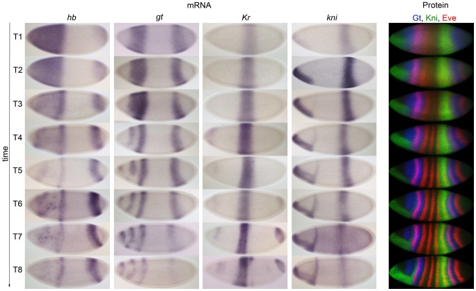
Figure 3 Comparison of mRNA and protein expression data: embryo images. Columns 1–4: time series of mRNA expression patterns of the trunk gap genes hb, gt, Kr and kni at cleavage cycle 14A (C14A) visualised by colorimetric (enzymatic) in situ hybridisation using wide-field microscopy. Column 5: time series of protein expression patterns of Gt, Kni and the pair-rule gene Even-skipped (Eve) at the equivalent developmental stages visualised by immunofluorescence using confocal laser scanning microscopy. Early stages at the top, time progresses downwards. Embryos are arranged anterior to the left, dorsal up. Embryos in column 5 are from the FlyEx database: http://urchin.spbcas.ru/flyex [69], [70]. T1–8 indicate time classes subdividing C14A (see Materials and Methods for details).
Figure 3 Comparison of mRNA and protein expression data: embryo images. Columns 1–4: time series of mRNA expression patterns of the trunk gap genes hb, gt, Kr and kni at cleavage cycle 14A (C14A) visualised by colorimetric (enzymatic) in situ hybridisation using wide-field microscopy. Column 5: time series of protein expression patterns of Gt, Kni and the pair-rule gene Even-skipped (Eve) at the equivalent developmental stages visualised by immunofluorescence using confocal laser scanning microscopy. Early stages at the top, time progresses downwards. Embryos are arranged anterior to the left, dorsal up. Embryos in column 5 are from the FlyEx database: http://urchin.spbcas.ru/flyex [69], [70]. T1–8 indicate time classes subdividing C14A (see Materials and Methods for details).CC BY · PubMed Central
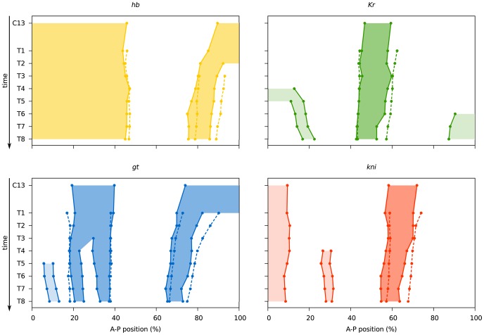
Figure 4 Comparison of mRNA and protein expression data: quantitative graphs. Space-time plots are shown indicating gap domain boundary positions based on mRNA (solid lines, shaded background) and protein data (dashed lines). Boundary positions for mRNA domains were determined as described for Table 2 (see also Materials and Methods). Boundary positions for gap protein domains are taken from [43]. Light shaded background indicates domains (the anterior domain of Kni, the anterior and posterior domains of Kr, and the head patch of Gt), which do not play a role in segment determination [35], and where not quantified from protein data in [43]. See also Table 2, and Tables S1 and S2.
Figure 4 Comparison of mRNA and protein expression data: quantitative graphs. Space-time plots are shown indicating gap domain boundary positions based on mRNA (solid lines, shaded background) and protein data (dashed lines). Boundary positions for mRNA domains were determined as described for Table 2 (see also Materials and Methods). Boundary positions for gap protein domains are taken from [43]. Light shaded background indicates domains (the anterior domain of Kni, the anterior and posterior domains of Kr, and the head patch of Gt), which do not play a role in segment determination [35], and where not quantified from protein data in [43]. See also Table 2, and Tables S1 and S2.CC BY · PubMed Central
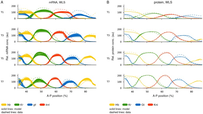
Figure 5 Gene circuit fits: model output versus data. Plots show model output (solid lines) versus expression data (dashed lines). (A) Gene circuits fit with WLS to mRNA data. All 52 selected gene circuits are shown. (B) Gene circuits fit with WLS to protein data (from [49]). All 66 selected gene circuits are shown. Horizontal axes represent A–P position (where 0% is the anterior pole). Relative mRNA and protein concentrations are in arbitrary units (au). T1/3/5/7 represent time classes during C14A; time progresses downwards.
Figure 5 Gene circuit fits: model output versus data. Plots show model output (solid lines) versus expression data (dashed lines). (A) Gene circuits fit with WLS to mRNA data. All 52 selected gene circuits are shown. (B) Gene circuits fit with WLS to protein data (from [49]). All 66 selected gene circuits are shown. Horizontal axes represent A–P position (where 0% is the anterior pole). Relative mRNA and protein concentrations are in arbitrary units (au). T1/3/5/7 represent time classes during C14A; time progresses downwards.CC BY · PubMed Central
Figure 6 Gene circuit analysis: mRNA- versus protein-based models. (A) Distribution of estimated parameter values (shown as scatter plots) for regulatory weights. Horizontal bars indicate the strength and type of interaction between regulators (indicated along the x-axes of the plots) and their target genes (sorted into separate plots). Blue represents parameter values from mRNA-based circuits, orange parameter values from protein-based circuits. (B) Genetic interconnectivity matrices indicating repressive (red), activating (green), or no (blue) interactions for WLS mRNA- (top) and protein-based gene circuits (bottom). Number triplets indicate the number of solutions with repressive/no/activating interactions. As in earlier studies [48], [49] a cut-off of 0.005 was used below which an interaction was considered to be absent. In cases where all gene circuits show identical behaviour, a dark colour is used; otherwise a lighter shade is applied. A black border highlights differences in interactions between the mRNA and protein circuits. (C) Regulatory contributions (calculated as regulator concentrations multiplied by regulatory weights or see equation 3) of gap genes and external inputs on gt (upper panel) and hb (lower panel) along the A–P axis (0% is the anterior pole). The horizontal dashed lines indicate threshold values (parameter in equation 3). The sum of positive contributions (above dashed line) is plotted separately from the sum of negative ones (below dashed line). The black curve indicates total regulatory effect: it is activating above the dashed line, and repressing below the dashed line. The posterior area of overlap (between vertical dashed lines) indicates where gt and hb have overlapping expression domains (the anterior overlap is omitted for clarity). To calculate the net interaction between gt and hb, the respective regulatory contributions are integrated over this area and the difference is calculated. The size of the coloured areas indicates a stronger repressive effect of Hb on gt than the other way around. (D) Consensus gap gene network recovered by both mRNA- and protein-based circuits. The position of gap domains is shown schematically along the A–P axis (coloured boxes). Background colour indicates predominant maternal activators. Circular arrows indicate auto-activation, T-bar connectors represent major repressive interactions, and dashed T-bar connectors show asymmetric repressive interactions determined by net effect (see panel C). See text for details.
Figure 6 Gene circuit analysis: mRNA- versus protein-based models. (A) Distribution of estimated parameter values (shown as scatter plots) for regulatory weights. Horizontal bars indicate the strength and type of interaction between regulators (indicated along the x-axes of the plots) and their target genes (sorted into separate plots). Blue represents parameter values from mRNA-based circuits, orange parameter values from protein-based circuits. (B) Genetic interconnectivity matrices indicating repressive (red), activating (green), or no (blue) interactions for WLS mRNA- (top) and protein-based gene circuits (bottom). Number triplets indicate the number of solutions with repressive/no/activating interactions. As in earlier studies [48], [49] a cut-off of 0.005 was used below which an interaction was considered to be absent. In cases where all gene circuits show identical behaviour, a dark colour is used; otherwise a lighter shade is applied. A black border highlights differences in interactions between the mRNA and protein circuits. (C) Regulatory contributions (calculated as regulator concentrations multiplied by regulatory weights or see equation 3) of gap genes and external inputs on gt (upper panel) and hb (lower panel) along the A–P axis (0% is the anterior pole). The horizontal dashed lines indicate threshold values (parameter in equation 3). The sum of positive contributions (above dashed line) is plotted separately from the sum of negative ones (below dashed line). The black curve indicates total regulatory effect: it is activating above the dashed line, and repressing below the dashed line. The posterior area of overlap (between vertical dashed lines) indicates where gt and hb have overlapping expression domains (the anterior overlap is omitted for clarity). To calculate the net interaction between gt and hb, the respective regulatory contributions are integrated over this area and the difference is calculated. The size of the coloured areas indicates a stronger repressive effect of Hb on gt than the other way around. (D) Consensus gap gene network recovered by both mRNA- and protein-based circuits. The position of gap domains is shown schematically along the A–P axis (coloured boxes). Background colour indicates predominant maternal activators. Circular arrows indicate auto-activation, T-bar connectors represent major repressive interactions, and dashed T-bar connectors show asymmetric repressive interactions determined by net effect (see panel C). See text for details.CC BY · PubMed Central
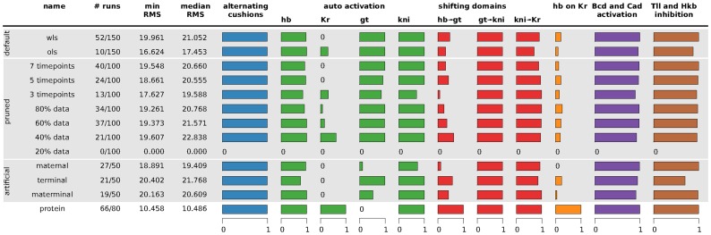
Figure 7 Summary of gene circuit performance under various scenarios of data availability. Scenario names are described in Table 4. Column 1–4: for each scenario, the number of selected/total runs is given; the minimum and median RMS score of the selected runs is indicated. The horizontal bar graphs to the right represent fractions of the selected runs in which specific regulatory mechanisms were found to be present. Smaller bars correspond to single interactions, larger to summaries of multiple interactions. Blue column: alternating cushions refers to the inhibiting interactions of hb and kni, as well as gt and Kr. Green columns: auto-activation is defined as a gene having an activating interaction with itself. Red columns: shifting domains are defined in terms of the following net effects between overlapping gap domains (see main text for the definition of net effects): posterior hb represses posterior gt, gt represses kni, and kni represses Kr (cf. Figure 6C). Orange column: the net repressive interaction between hb and Kr, as calculated for other overlapping gag domains above. Bars indicate net repression of Kr by Hb, which is the standard situation in protein-based circuits, while most mRNA-based circuits show net repression of hb by Kr. Purple column: Bcd and Cad activation is defined as the fraction of gene circuits in which Bcd activates all four gap genes and Cad activates gt and kni. Brown column: Tll and Hkb inhibition is defined as Hkb inhibiting hb, while Tll inhibits the other three gap genes. See text for details. The results summarised here are based on the interconnectivity matrices shown in Text S3.
Figure 7 Summary of gene circuit performance under various scenarios of data availability. Scenario names are described in Table 4. Column 1–4: for each scenario, the number of selected/total runs is given; the minimum and median RMS score of the selected runs is indicated. The horizontal bar graphs to the right represent fractions of the selected runs in which specific regulatory mechanisms were found to be present. Smaller bars correspond to single interactions, larger to summaries of multiple interactions. Blue column: alternating cushions refers to the inhibiting interactions of hb and kni, as well as gt and Kr. Green columns: auto-activation is defined as a gene having an activating interaction with itself. Red columns: shifting domains are defined in terms of the following net effects between overlapping gap domains (see main text for the definition of net effects): posterior hb represses posterior gt, gt represses kni, and kni represses Kr (cf. Figure 6C). Orange column: the net repressive interaction between hb and Kr, as calculated for other overlapping gag domains above. Bars indicate net repression of Kr by Hb, which is the standard situation in protein-based circuits, while most mRNA-based circuits show net repression of hb by Kr. Purple column: Bcd and Cad activation is defined as the fraction of gene circuits in which Bcd activates all four gap genes and Cad activates gt and kni. Brown column: Tll and Hkb inhibition is defined as Hkb inhibiting hb, while Tll inhibits the other three gap genes. See text for details. The results summarised here are based on the interconnectivity matrices shown in Text S3.CC BY · PubMed Central

Verification

Claims the paper makes

The claims and statistics of this paper haven’t been checked yet.

Free: it reads the open-access text and checks the first 5 claims that cite a source we can check. Create a free account to check every claim.

A few free checks a day · papers already verified open instantly · results are public

Claims other papers make about this one

Each is checked against this paper’s own text: does it say what the citing paper says it does?

Self-check

Percentages, sums and reported differences re-computed from the paper’s own numbers.

The self-check needs the paper’s full text.

Citations

Cites

Show all 111 references

Research works printed but not linked: 2

  1. J Lam, 1988, An efficient simulated annealing schedule: derivation. New Haven, CT: Yale Electrical Engineering Department., Technical Report, 8816
  2. J Lam, 1988, An efficient simulated annealing schedule: implementation and evaluation. New Haven, CT: Yale Electrical Engineering Department., Technical Report, 8817

Cited by

See all 83

Metadata

Authors
Crombach, A., Wotton, K. R., Cicin-Sain, D., Ashyraliyev, M., & Jaeger, J.
Affiliations
  • Universitat Pompeu Fabra (ES)
  • Bahçeşehir University (TR)
Corresponding author
Jaeger, Johannes
Venue
PLoS Computational Biology
Published
2012-07-12
Volume
8
Issue
7
Pages
e1002589
ISSN
  • 1553-734X (ISSN-L)
  • 1553-7358
OpenAlex
W2051676319
Cited by
83
References
113
Citations by year
2026: 1 · 2025: 1 · 2024: 3 · 2023: 4 · 2022: 1 · 2021: 4 · 2020: 4 · 2019: 4 · 2018: 4 · 2017: 8 · 2016: 9 · 2015: 13 · 2014: 14 · 2013: 11 · 2012: 2
FWCI
5.15
Type
journal article
Language
en
Open access
Locations
  • PLoS Computational Biology (publishedVersion, cc-by)
  • Europe PMC (PubMed Central) (publishedVersion, cc-by)
  • PubMed Central (publishedVersion, cc-by)
  • PubMed (publishedVersion)
  • DOAJ (DOAJ: Directory of Open Access Journals) (submittedVersion, cc-by-sa)
  • Figshare (submittedVersion, cc-by)
  • Figshare (submittedVersion)
  • Open Research Exeter (University of Exeter) (submittedVersion, other-oa)
Funders
  • European Commission (KBBE-2011-5, FP7-KBBE-2011–5, 289434, FP7-KBBE)
  • Ministerio de Economía y Competitividad (BFU2009-10184)
  • Agència de Gestió d'Ajuts Universitaris i de Recerca (BFU2009-10184, SGR Grant 406)
  • FP7 Food, Agriculture and Fisheries, Biotechnology (289434)
Topics
  • Life Sciences › Biochemistry, Genetics and Molecular Biology › Molecular Biology › Gene Regulatory Network Analysis
  • Life Sciences › Biochemistry, Genetics and Molecular Biology › Molecular Biology › Developmental Biology and Gene Regulation
  • Life Sciences › Biochemistry, Genetics and Molecular Biology › Molecular Biology › Genomics and Chromatin Dynamics
Keywords
gene regulatory network inference, reverse engineering, Drosophila melanogaster, spatial gene expression, developmental gene regulation
MeSH terms
Animals, Computer Simulation, Drosophila melanogaster, Hybridization, Genetic, Models, Genetic, RNA, Messenger, Gene Expression, Genes, Insect, Computational Biology, Drosophila Proteins, Gene Regulatory Networks

About these checks

Registry, retraction, Cites and statistics results are computed, not judged, with one exception: a printed reference that no index lists is read once by a model before it counts as a citation error. Claims are extracted by a model and kept only when their quote appears verbatim in the text; each cited source is then checked, with a model’s help, for whether it says what the claim relies on. Those verdicts can be wrong — read the claim’s quote and the cited source before relying on one.

Statistics and arithmetic are recomputed, not judged.

Confidence bands are shown only for fields calibrated on our annotated test set. None is calibrated yet, so no band is shown.

What counts as a claim ›How we measure confidence ›How we check this ›

Are you an author, or do you see a problem with this page? Request a review

How to cite

Cite CoChat for the checks on this page, and the paper for its own findings.

This page
CoChat. (2026). Citation check: Efficient Reverse-Engineering of a Developmental Gene Regulatory Network. https://app.cochat.ai/papers/10.1371/journal.pcbi.1002589
The paper
Crombach, A., Wotton, K. R., Cicin-Sain, D., Ashyraliyev, M., & Jaeger, J. (2012). Efficient Reverse-Engineering of a Developmental Gene Regulatory Network. PLoS Computational Biology. https://doi.org/10.1371/journal.pcbi.1002589

Data sources

Bibliographic data: Semantic Scholar, OpenAlex, Crossref.

Contains information from the Semantic Scholar Academic Graph Datasets, made available under the ODC Attribution License (ODC-BY 1.0).

Semantic Scholar’s data is described in: Kinney, R., et al. (2023). The Semantic Scholar Open Data Platform. arXiv:2301.10140.