Cited by 385Statistical Methods and Bayesian InferenceControl Systems and IdentificationGaussian Processes and Bayesian Inference

The DOI matches its Crossref record; 40 of the 41 references it cites were found in a registry or an index.

VBA: A Probabilistic Treatment of Nonlinear Models for Neurobiological and Behavioural Data

Open access
Daunizeau, Jean, Adam, Vincent, Rigoux, Lionel·2014·PLoS Computational Biology

Abstract

This work is in line with an on-going effort tending toward a computational (quantitative and refutable) understanding of human neuro-cognitive processes. Many sophisticated models for behavioural and neurobiological data have flourished during the past decade. Most of these models are partly unspecified (i.e. they have unknown parameters) and nonlinear. This makes them difficult to peer with a formal statistical data analysis framework. In turn, this compromises the reproducibility of model-based empirical studies. This work exposes a software toolbox that provides generic, efficient and robust probabilistic solutions to the three problems of model-based analysis of empirical data: (i) data simulation, (ii) parameter estimation/model selection, and (iii) experimental design optimization.

Overview

The claims and statistics of this paper haven’t been checked yet.

Run the check — free, no account needed. It reads the open-access text and checks the sources it cites.

A few free checks a day · papers already verified open instantly · results are public

Integrity signals

Registry

Crossref · 10.1371/journal.pcbi.1003441

Cites

40 of 40 references verified0 citation errors · 0 not checkable

Statistics

Figures

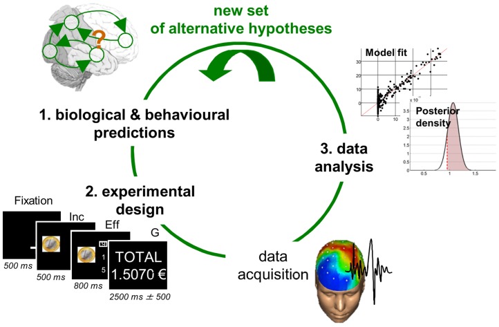
Figure 1 The experimental cycle. The experimental cycle summarizes the interaction between modelling, experimental work and statistical data analysis. One starts with new competing hypotheses about a system of interest. These are then embodied into a set of candidate models that are to be compared with each other given empirical data. One then designs an experiment that is maximally discriminative with respect to the candidate models. Data acquisition and analysis then proceed, the conclusion of which serves to generate a new set of competing hypotheses, etc… Adapted from [14].
Figure 1 The experimental cycle. The experimental cycle summarizes the interaction between modelling, experimental work and statistical data analysis. One starts with new competing hypotheses about a system of interest. These are then embodied into a set of candidate models that are to be compared with each other given empirical data. One then designs an experiment that is maximally discriminative with respect to the candidate models. Data acquisition and analysis then proceed, the conclusion of which serves to generate a new set of competing hypotheses, etc… Adapted from [14].CC BY · PubMed Central
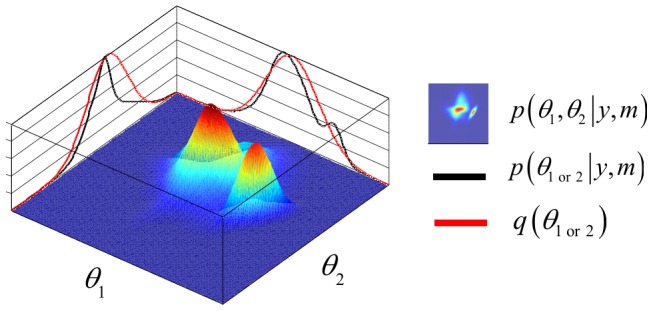
Figure 2 The mean-field/Laplace approximation. The variational Bayesian approach furnishes an approximation to the marginal posterior densities of subsets of unknown model parameters . Here, the 2D landscape depicts a (true) joint posterior density and the two black lines are the subsequent marginal posterior densities of and , respectively. The mean-field approximation basically describes the joint posterior density as the product of the two marginal densities (black profiles). In turn, stochastic dependencies between parameter subsets are replaced by deterministic dependencies between their posterior sufficient statistics. The Laplace approximation further assumes that the marginal densities can be described by Gaussian densities (red profiles).
Figure 2 The mean-field/Laplace approximation. The variational Bayesian approach furnishes an approximation to the marginal posterior densities of subsets of unknown model parameters . Here, the 2D landscape depicts a (true) joint posterior density and the two black lines are the subsequent marginal posterior densities of and , respectively. The mean-field approximation basically describes the joint posterior density as the product of the two marginal densities (black profiles). In turn, stochastic dependencies between parameter subsets are replaced by deterministic dependencies between their posterior sufficient statistics. The Laplace approximation further assumes that the marginal densities can be described by Gaussian densities (red profiles).CC BY · PubMed Central
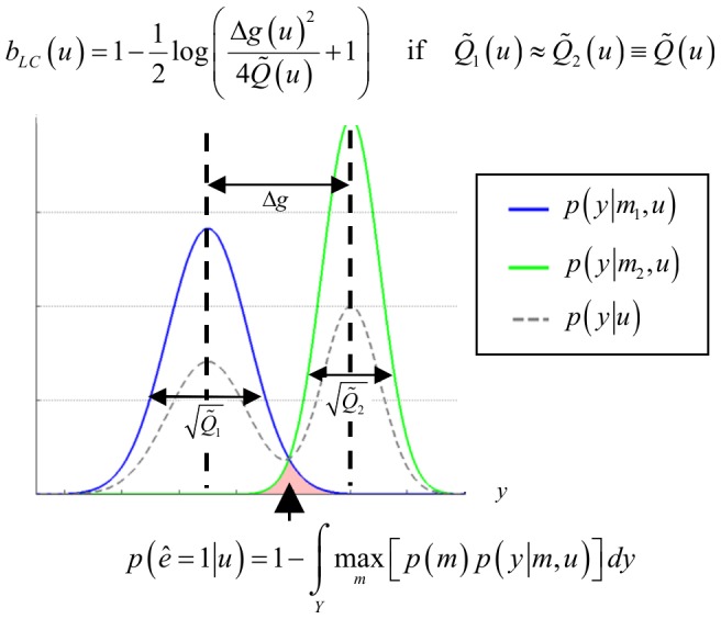
Figure 3 Selection error rate and the Laplace-Chernoff risk. The (univariate) prior predictive density of two generative models (blue) and (green) are plotted as a function of data y, given an arbitrary design u. The dashed grey line shows the marginal predictive density that captures the probabilistic prediction of the whole comparison set . The area under the curve (red) measures the model selection error rate , which depends upon the discriminability between the two prior predictive density and . This is precisely what the Laplace-Chernoff risk is a measure of. Adapted from [14].
Figure 3 Selection error rate and the Laplace-Chernoff risk. The (univariate) prior predictive density of two generative models (blue) and (green) are plotted as a function of data y, given an arbitrary design u. The dashed grey line shows the marginal predictive density that captures the probabilistic prediction of the whole comparison set . The area under the curve (red) measures the model selection error rate , which depends upon the discriminability between the two prior predictive density and . This is precisely what the Laplace-Chernoff risk is a measure of. Adapted from [14].CC BY · PubMed Central
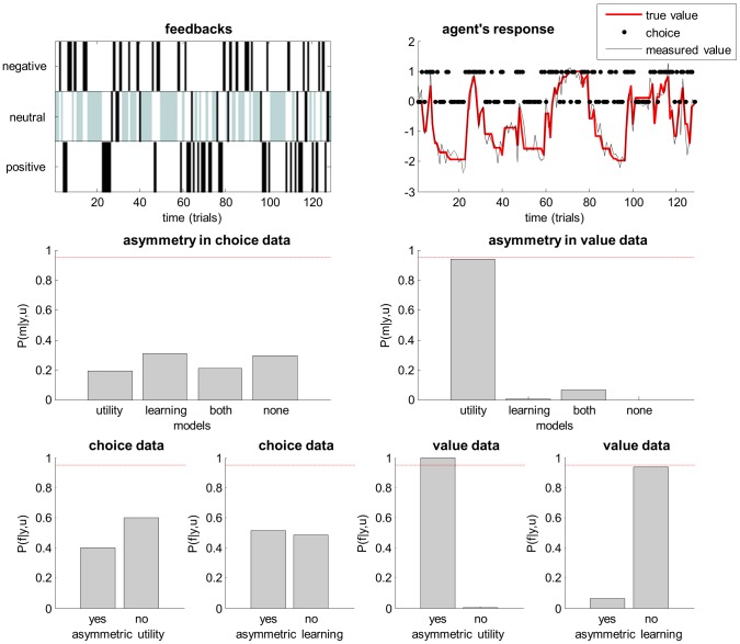
Figure 4 Comparison of asymmetric utility and asymmetric learning rate. This figure summarizes the analysis of choice and value data using models that assume asymmetric utility, asymmetric learning rate, both asymmetries or none. Upper left: Trial-by-trial feedback history (either negative, neutral or positive). Grey neutral feedbacks correspond to ‘no-go’ choices. Upper right: Trial-by-trial dynamics of true value (red), measured value (black) and agent's binary go(1)/no-go(0) choices (black dots). Middle-left: posterior probability of the four models given simulated choice data. Middle-right: same format, given value data. Lower left: family posterior probabilities for both model spaces partitions, given choice data (left: family ‘yes’ = {‘utility’, ‘both’} vs family ‘no’ = {‘learning’, ‘none’}, right: family ‘yes’ = {‘learning’, ‘both’} vs family ‘no’ = {‘utility’, none’}. Lower left: same format, given value data.
Figure 4 Comparison of asymmetric utility and asymmetric learning rate. This figure summarizes the analysis of choice and value data using models that assume asymmetric utility, asymmetric learning rate, both asymmetries or none. Upper left: Trial-by-trial feedback history (either negative, neutral or positive). Grey neutral feedbacks correspond to ‘no-go’ choices. Upper right: Trial-by-trial dynamics of true value (red), measured value (black) and agent's binary go(1)/no-go(0) choices (black dots). Middle-left: posterior probability of the four models given simulated choice data. Middle-right: same format, given value data. Lower left: family posterior probabilities for both model spaces partitions, given choice data (left: family ‘yes’ = {‘utility’, ‘both’} vs family ‘no’ = {‘learning’, ‘none’}, right: family ‘yes’ = {‘learning’, ‘both’} vs family ‘no’ = {‘utility’, none’}. Lower left: same format, given value data.CC BY · PubMed Central
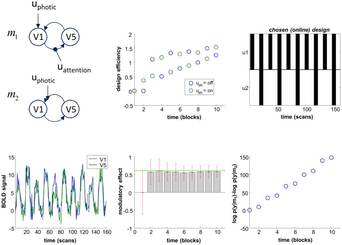
Figure 5 Online design optimization for DCM comparison. This figure summarizes the simulation of online design optimization, in the aim of best discriminating between two brain network models ( and ) given fMRI data time series. In this case, the problem reduces to deciding whether or not to introduce the second experimental factor (here, = attentional modulation), on top of the first factor ( = photic stimulation). Upper left: the two network models to be compared given fMRI data (top/bottom: with/without attentional modulation of the V1→V5 connection). Upper middle: block-by-block temporal dynamics of design efficiency of both types of blocks. Green (resp. blue) dots correspond to blocks with (resp. without.) attentional modulation. Upper right: scan-by-scan temporal dynamics of the optimized (on-line) design. Lower left: scan-by-scan temporal dynamics of the simulated fMRI signal (blue: V1, green: V5). Lower middle: block-by-block temporal dynamics of 95% posterior confidence intervals on the estimated modulatory effect (under model ). The green line depicts the strength of the simulated effect. Lower right: block-by-block temporal dynamics of log Bayes factors .
Figure 5 Online design optimization for DCM comparison. This figure summarizes the simulation of online design optimization, in the aim of best discriminating between two brain network models ( and ) given fMRI data time series. In this case, the problem reduces to deciding whether or not to introduce the second experimental factor (here, = attentional modulation), on top of the first factor ( = photic stimulation). Upper left: the two network models to be compared given fMRI data (top/bottom: with/without attentional modulation of the V1→V5 connection). Upper middle: block-by-block temporal dynamics of design efficiency of both types of blocks. Green (resp. blue) dots correspond to blocks with (resp. without.) attentional modulation. Upper right: scan-by-scan temporal dynamics of the optimized (on-line) design. Lower left: scan-by-scan temporal dynamics of the simulated fMRI signal (blue: V1, green: V5). Lower middle: block-by-block temporal dynamics of 95% posterior confidence intervals on the estimated modulatory effect (under model ). The green line depicts the strength of the simulated effect. Lower right: block-by-block temporal dynamics of log Bayes factors .CC BY · PubMed Central
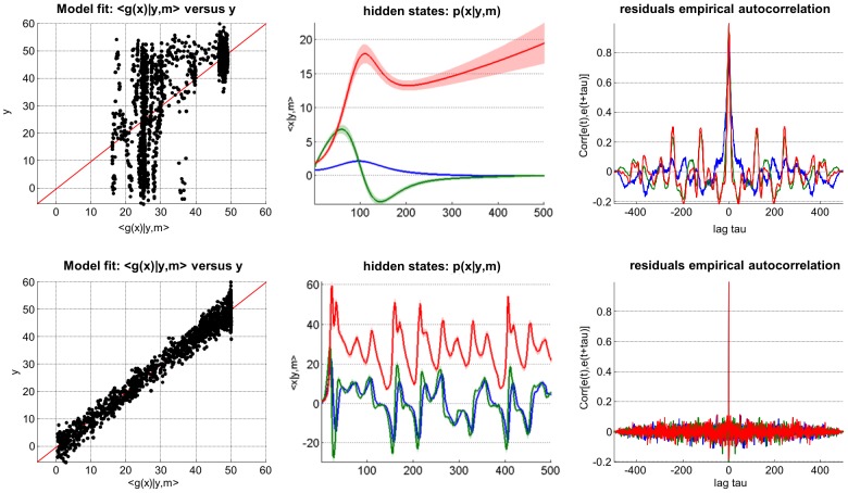
Figure 6 Comparison of deterministic and stochastic dynamical systems. This figure summarizes the VB comparison of deterministic (upper row) and stochastic (lower row) variants of a Lorenz dynamical system, given data simulated under the stochastic variant of the model. Upper left: fitted data (x-axis) is plotted against simulated data (y-axis), for the deterministic case. Perfect model fit would align all points on the red line. Lower left: same format, for the stochastic case. Upper middle: 95% posterior confidence intervals on hidden-states dynamics. Recall that for deterministic systems, uncertainty in the hidden states arises from evolution parameters' uncertainty. Lower middle: same format, stochastic system. Upper right: residuals' empirical autocorrelation (y-axis) as a function of temporal lag (x-axis), for the deterministic system. Lower right: same format, stochastic system.
Figure 6 Comparison of deterministic and stochastic dynamical systems. This figure summarizes the VB comparison of deterministic (upper row) and stochastic (lower row) variants of a Lorenz dynamical system, given data simulated under the stochastic variant of the model. Upper left: fitted data (x-axis) is plotted against simulated data (y-axis), for the deterministic case. Perfect model fit would align all points on the red line. Lower left: same format, for the stochastic case. Upper middle: 95% posterior confidence intervals on hidden-states dynamics. Recall that for deterministic systems, uncertainty in the hidden states arises from evolution parameters' uncertainty. Lower middle: same format, stochastic system. Upper right: residuals' empirical autocorrelation (y-axis) as a function of temporal lag (x-axis), for the deterministic system. Lower right: same format, stochastic system.CC BY · PubMed Central
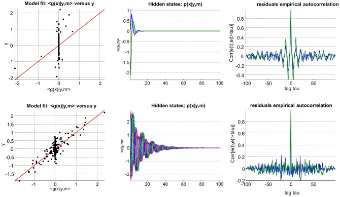
Figure 7 Comparison of delayed and non-delayed dynamical systems. This figure summarizes the VB comparison of non-delayed (upper row) and delayed (lower row) variants of a linear deterministic dynamical system, given data simulated under the delayed variant of the model. This figure uses the same format as Figure 6.
Figure 7 Comparison of delayed and non-delayed dynamical systems. This figure summarizes the VB comparison of non-delayed (upper row) and delayed (lower row) variants of a linear deterministic dynamical system, given data simulated under the delayed variant of the model. This figure uses the same format as Figure 6.CC BY · PubMed Central
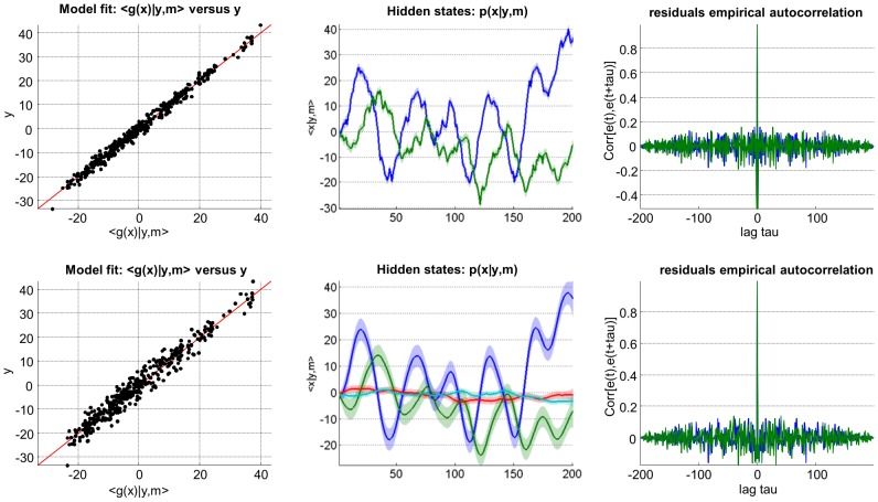
Figure 8 Comparison of white and auto-correlated state-noise. This figure summarizes the VB comparison of stochastic systems driven with either white (upper row) or auto-correlated (lower row) state noise. This figure uses the same format as Figure 6.
Figure 8 Comparison of white and auto-correlated state-noise. This figure summarizes the VB comparison of stochastic systems driven with either white (upper row) or auto-correlated (lower row) state noise. This figure uses the same format as Figure 6.CC BY · PubMed Central
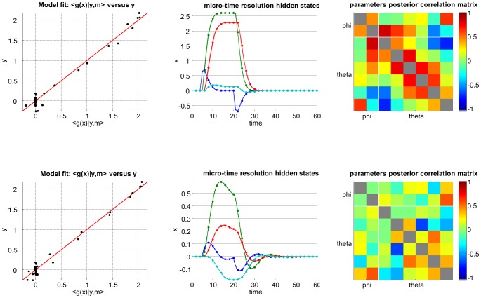
Figure 9 Effect of the micro-time resolution. This figure summarizes the effect of relying on either a slow (upper row) or fast (lower row) micro-time resolution, when inverting nonlinear dynamical systems. Left: same format as Figure 6. Upper middle: estimated hidden-states dynamics at low micro-time resolution (data samples are depicted using dots). Lower middle: same format, fast micro-time resolution. Upper right: parameters' posterior correlation matrix, at low micro-time resolution. Lower middle: same format, fast micro-time resolution.
Figure 9 Effect of the micro-time resolution. This figure summarizes the effect of relying on either a slow (upper row) or fast (lower row) micro-time resolution, when inverting nonlinear dynamical systems. Left: same format as Figure 6. Upper middle: estimated hidden-states dynamics at low micro-time resolution (data samples are depicted using dots). Lower middle: same format, fast micro-time resolution. Upper right: parameters' posterior correlation matrix, at low micro-time resolution. Lower middle: same format, fast micro-time resolution.CC BY · PubMed Central
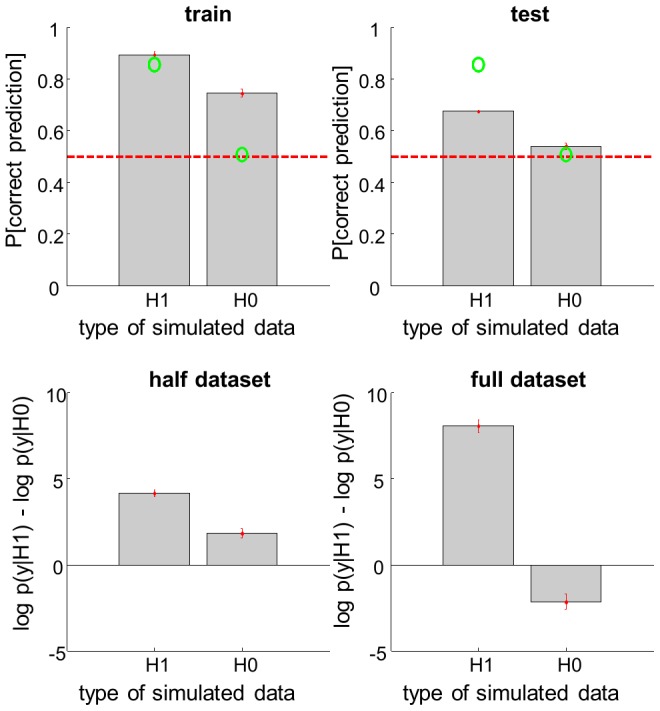
Figure 10 Binary data classification. This figure exemplifies a classification analysis, which is used to infer on the link between a continuous variable X and a binary data y. The analysis is conducted on data simulated under either a null model (H0: no link) or a sigmoid mapping (H1). Upper left: the classification accuracy, in terms of the Monte-Carlo average probability of correct prediction under both types of data (left: H1, right: H0), for the training dataset. The green dots show the expected classification accuracy, using the true values of each model's set of parameters. The dotted red line depicts chance level. Upper right: same format, test dataset (no model fitting). Lower left: same format, for the log Bayes factor , given the training dataset. Lower right: same format, given the full (train+test) dataset.
Figure 10 Binary data classification. This figure exemplifies a classification analysis, which is used to infer on the link between a continuous variable X and a binary data y. The analysis is conducted on data simulated under either a null model (H0: no link) or a sigmoid mapping (H1). Upper left: the classification accuracy, in terms of the Monte-Carlo average probability of correct prediction under both types of data (left: H1, right: H0), for the training dataset. The green dots show the expected classification accuracy, using the true values of each model's set of parameters. The dotted red line depicts chance level. Upper right: same format, test dataset (no model fitting). Lower left: same format, for the log Bayes factor , given the training dataset. Lower right: same format, given the full (train+test) dataset.CC BY · PubMed Central
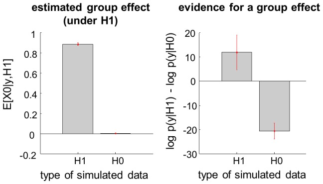
Figure 11 Random-effect analysis. This figure exemplifies a random-effect GLM analysis, which is used to infer on the group mean of an effect of interest. The analysis is conducted on data simulated under either a null model (H0: group mean is zero) or a non-zero RFX model (H1). Left: Monte-Carlo average of the VB-estimated group mean under H1, given both types of data (left: H1, right: H0). Left: same format, for the log Bayes factor .
Figure 11 Random-effect analysis. This figure exemplifies a random-effect GLM analysis, which is used to infer on the group mean of an effect of interest. The analysis is conducted on data simulated under either a null model (H0: group mean is zero) or a non-zero RFX model (H1). Left: Monte-Carlo average of the VB-estimated group mean under H1, given both types of data (left: H1, right: H0). Left: same format, for the log Bayes factor .CC BY · PubMed Central
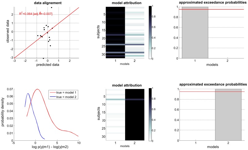
Figure 12 Random-effect group-BMS. This figure exemplifies a random-effect group-BMS analysis, which is used to infer on the best model at the group level. The analysis is conducted on two groups of 32 subjects, whose data were simulated under either a ‘full’ (, group 1) or a ‘reduced’ (, group 2) model. Upper left: simulated data (y-axis) plotted against fitted data (x-axis), for a typical simulation. Lower left: histograms of log Bayes factor , for both groups (red: group 1, blue: group 2). Upper middle: model attributions, for group 1. The posterior probability for each subject is coded on a black-and-white colour scale (black = 1, white = 0). Lower middle: same format, group 2. Upper right: exceedance probabilities, for group 1. The red line indicates the usual 95% threshold. Lower right: same format, group 2.
Figure 12 Random-effect group-BMS. This figure exemplifies a random-effect group-BMS analysis, which is used to infer on the best model at the group level. The analysis is conducted on two groups of 32 subjects, whose data were simulated under either a ‘full’ (, group 1) or a ‘reduced’ (, group 2) model. Upper left: simulated data (y-axis) plotted against fitted data (x-axis), for a typical simulation. Lower left: histograms of log Bayes factor , for both groups (red: group 1, blue: group 2). Upper middle: model attributions, for group 1. The posterior probability for each subject is coded on a black-and-white colour scale (black = 1, white = 0). Lower middle: same format, group 2. Upper right: exceedance probabilities, for group 1. The red line indicates the usual 95% threshold. Lower right: same format, group 2.CC BY · PubMed Central
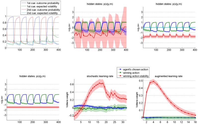
Figure 13 Improving Q-learning models with inversion diagnostics. This figure demonstrates the added-value of Volterra decompositions, when deriving learning models with changing learning rates. Upper left: simulated belief (blue/red: outcome probability for the first/second action, green/magenta: volatility of the outcome contingency for the first/second action) of the Bayesian volatile learner (y-axis) plotted against trials (x-axis). Lower left: estimated hidden states of the deterministic variant of the dynamic learning rate model (blue/green: first/second action value, red: learning rate). This model corresponds to the standard Q-learning model (the learning rate is constant over time). Upper middle: estimated hidden states of the stochastic variant of the dynamic learning rate model (same format). Note the wide posterior uncertainty around the learning rate estimates. Lower middle: Volterra decomposition of the stochastic learning rate (blue: agent's chosen action, green: winning action, red: winning action instability). Upper right: estimated hidden states of the augmented Q-learning model (same format as before). Lower right: Volterra decomposition of the augmented Q-learning model's learning rate (same format as before).
Figure 13 Improving Q-learning models with inversion diagnostics. This figure demonstrates the added-value of Volterra decompositions, when deriving learning models with changing learning rates. Upper left: simulated belief (blue/red: outcome probability for the first/second action, green/magenta: volatility of the outcome contingency for the first/second action) of the Bayesian volatile learner (y-axis) plotted against trials (x-axis). Lower left: estimated hidden states of the deterministic variant of the dynamic learning rate model (blue/green: first/second action value, red: learning rate). This model corresponds to the standard Q-learning model (the learning rate is constant over time). Upper middle: estimated hidden states of the stochastic variant of the dynamic learning rate model (same format). Note the wide posterior uncertainty around the learning rate estimates. Lower middle: Volterra decomposition of the stochastic learning rate (blue: agent's chosen action, green: winning action, red: winning action instability). Upper right: estimated hidden states of the augmented Q-learning model (same format as before). Lower right: Volterra decomposition of the augmented Q-learning model's learning rate (same format as before).CC BY · PubMed Central

Verification

Claims the paper makes

The claims and statistics of this paper haven’t been checked yet.

Run the check — free, no account needed. It reads the open-access text and checks the sources it cites.

A few free checks a day · papers already verified open instantly · results are public

Claims other papers make about this one

Each is checked against this paper’s own text: does it say what the citing paper says it does?

Self-check

Percentages, sums and reported differences re-computed from the paper’s own numbers.

The self-check needs the paper’s full text.

Citations

Cites

Show all 41 references

Research works printed but not linked: 1

  1. Robert C. (2007), The Bayesian choice: From Decision-Theoretic Foundations to Computational Implementation. Springer, August 2007.

Cited by

Sorted by citations

See all 385

Metadata

Authors
Daunizeau, J., Adam, V., & Rigoux, L.
Affiliations
  • Gatsby Computational Neuroscience Unit (GB)
  • Institut du Cerveau (FR)
Venue
PLoS Computational Biology
Published
2014-01-23
Volume
10
Issue
1
Pages
e1003441
ISSN
  • 1553-734X (ISSN-L)
  • 1553-7358
OpenAlex
W2049657715
Cited by
385
References
41
Citations by year
2026: 28 · 2025: 36 · 2024: 44 · 2023: 37 · 2022: 39 · 2021: 47 · 2020: 47 · 2019: 24 · 2018: 22 · 2017: 24 · 2016: 21 · 2015: 7 · 2014: 9
FWCI
21.23
Type
journal article
Language
en
Open access
Locations
  • PLoS Computational Biology (publishedVersion, cc-by)
  • Europe PMC (PubMed Central) (publishedVersion, cc-by)
  • PubMed Central (publishedVersion, cc-by)
  • PubMed (publishedVersion)
  • RePEc: Research Papers in Economics (submittedVersion)
  • DOAJ (DOAJ: Directory of Open Access Journals) (submittedVersion)
  • Figshare (submittedVersion, cc-by)
Topics
  • Physical Sciences › Mathematics › Statistics and Probability › Statistical Methods and Bayesian Inference
  • Physical Sciences › Engineering › Control and Systems Engineering › Control Systems and Identification
  • Physical Sciences › Computer Science › Artificial Intelligence › Gaussian Processes and Bayesian Inference
Keywords
stochastic modeling, nonlinear models, parameter estimation, model selection, data simulation, experimental design optimization, behavioral data, computational neuroscience, reproducibility
MeSH terms
Algorithms, Bayes Theorem, Cognition, Computer Simulation, Decision Making, Humans, Models, Biological, Models, Neurological, Nerve Net, Probability, Software, Stochastic Processes, Normal Distribution, Computational Biology

About these checks

Registry, retraction, Cites and statistics results are computed, not judged, with one exception: a printed reference that no index lists is read once by a model before it counts as a citation error. Claims are extracted by a model and kept only when their quote appears verbatim in the text; each cited source is then checked, with a model’s help, for whether it says what the claim relies on. Those verdicts can be wrong — read the claim’s quote and the cited source before relying on one.

Statistics and arithmetic are recomputed, not judged.

Confidence bands are shown only for fields calibrated on our annotated test set. None is calibrated yet, so no band is shown.

What counts as a claim ›How we measure confidence ›How we check this ›

Are you an author, or do you see a problem with this page? Request a review