

Deep Supervised, but Not Unsupervised, Models May Explain IT Cortical Representation
Open accessThe DOI matches its Crossref record; 99 of the 99 references it cites were found in a registry or an index.
Abstract
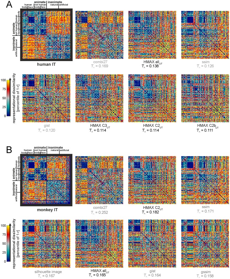
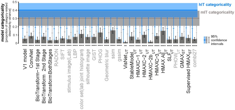
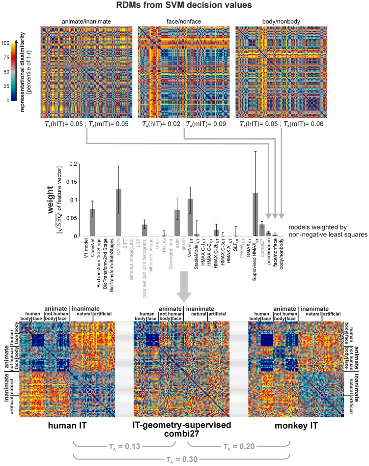
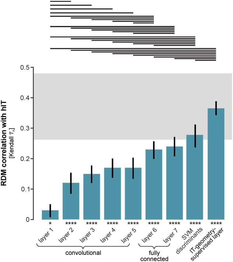
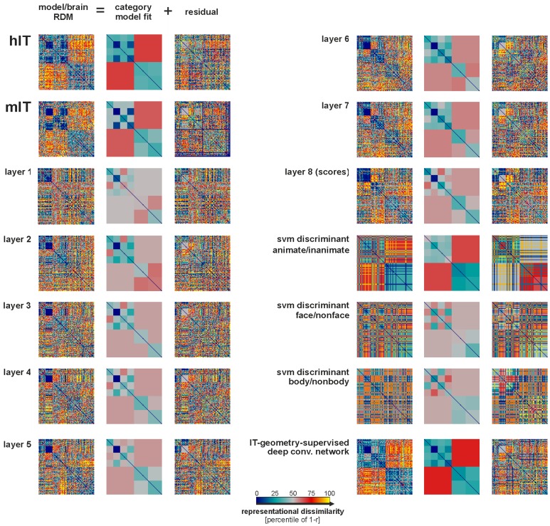
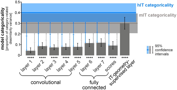
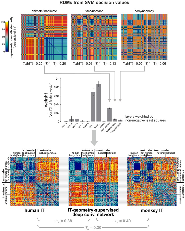
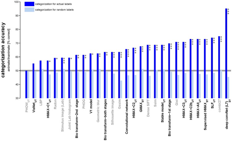
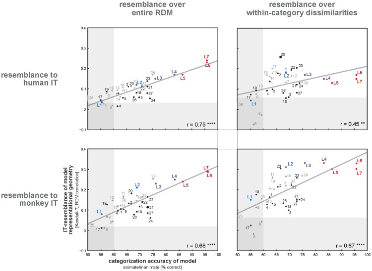
Inferior temporal (IT) cortex in human and nonhuman primates serves visual object recognition. Computational object-vision models, although continually improving, do not yet reach human performance. It is unclear to what extent the internal representations of computational models can explain the IT representation. Here we investigate a wide range of computational model representations (37 in total), testing their categorization performance and their ability to account for the IT representational geometry. The models include well-known neuroscientific object-recognition models (e.g. HMAX, VisNet) along with several models from computer vision (e.g. SIFT, GIST, self-similarity features, and a deep convolutional neural network). We compared the representational dissimilarity matrices (RDMs) of the model representations with the RDMs obtained from human IT (measured with fMRI) and monkey IT (measured with cell recording) for the same set of stimuli (not used in training the models). Better performing models were more similar to IT in that they showed greater clustering of representational patterns by category. In addition, better performing models also more strongly resembled IT in terms of their within-category representational dissimilarities. Representational geometries were significantly correlated between IT and many of the models. However, the categorical clustering observed in IT was largely unexplained by the unsupervised models. The deep convolutional network, which was trained by supervision with over a million category-labeled images, reached the highest categorization performance and also best explained IT, although it did not fully explain the IT data. Combining the features of this model with appropriate weights and adding linear combinations that maximize the margin between animate and inanimate objects and between faces and other objects yielded a representation that fully explained our IT data. Overall, our results suggest that explaining IT requires computational features trained through supervised learning to emphasize the behaviorally important categorical divisions prominently reflected in IT.
Overview
The claims and statistics of this paper haven’t been checked yet.
Free: it reads the open-access text and checks the first 5 claims that cite a source we can check. Create a free account to check every claim.
Integrity signals
Registry
Cites
Statistics
Figures



Verification
Claims the paper makes
The claims and statistics of this paper haven’t been checked yet.
Free: it reads the open-access text and checks the first 5 claims that cite a source we can check. Create a free account to check every claim.
Claims other papers make about this one
Each is checked against this paper’s own text: does it say what the citing paper says it does?
The cited source says what the claim attributes to it.
In the citing paper
“Using this approach, known as neuroconnectionism, numerous studies have identified shared representational structure across brains and ANN models, as well as factors influencing this alignment [5–11]”
From The Umwelt Representation Hypothesis: rethinking Universality (2026) · cites this paper as [10]
The cited source says what the claim attributes to it.
In the citing paper
“Analogous approaches have proven successful in relating the structure of neural activity to computational functions in other domains, including vision 17–19, audition 20, olfaction 21,22, thermosensation 23, perceptual discrimination 24, facial perception 25, and navigation 26,27.”
From A virtual rodent predicts the structure of neural activity across behaviours (2024) · cites this paper as [19]
Self-check
Percentages, sums and reported differences re-computed from the paper’s own numbers.
The self-check needs the paper’s full text.
Citations
Cites
ImageNet classification with deep convolutional neural networks
Krizhevsky, A., Sutskever, I., & Hinton, G. E. (2017) · Communications of the ACM · doi:10.1145/3065386 · Cited by 112,155
ImageNet: A large-scale hierarchical image database
Deng, J., Dong, W., Socher, R., Li, L.-J., Li, K., & Fei-Fei, L. (2009) · 2009 IEEE Conference on Computer Vision and Pattern Recognition · doi:10.1109/cvpr.2009.5206848 · Cited by 65,333 · cited 2×
“This is a supervised convolutional neural network, trained with 1.2 million labelled images from ImageNet (1000 category labels) [52].”
MethodInfluentialDistinctive Image Features from Scale-Invariant Keypoints
Lowe, D. G. (2004) · International Journal of Computer Vision · doi:10.1023/b:visi.0000029664.99615.94 · Cited by 55,589
LIBSVM: A library for support vector machines
Chang, C.-C., & Lin, C.-J. (2011) · ACM Transactions on Intelligent Systems and Technology · doi:10.1145/1961189.1961199 · Cited by 40,918
Object recognition from local scale-invariant features
Lowe, D. G. (1999) · Proceedings of the Seventh IEEE International Conference on Computer Vision · doi:10.1109/iccv.1999.790410 · Cited by 16,472
A fast learning algorithm for deep belief nets
Hinton, G. E., Osindero, S., & Teh, Y.-W. (2006) · Neural Computation · doi:10.1162/neco.2006.18.7.1527 · Cited by 16,336
Visualizing and understanding convolutional networks
Zeiler, M. D., & Fergus, R. (2014) · Lecture Notes in Computer Science · doi:10.1007/978-3-319-10590-1_53 · Cited by 15,839
Multiresolution gray-scale and rotation invariant texture classification with local binary patterns
Ojala, T., Pietikainen, M., & Maenpaa, T. (2002) · IEEE Transactions on Pattern Analysis and Machine Intelligence · doi:10.1109/tpami.2002.1017623 · Cited by 15,398
Receptive fields, binocular interaction and functional architecture in the cat’s visual cortex
Hubel, D. H., & Wiesel, T. N. (1962) · The Journal of Physiology · doi:10.1113/jphysiol.1962.sp006837 · Cited by 13,680
Libsvm : A library for support vector machines
Ferrari, V. (2008) · Medical Entomology and Zoology · Cited by 10,122
Learning Deep Architectures for AI
Bengio, Y. (2009) · Foundations and Trends® in Machine Learning · doi:10.1561/2200000006 · Cited by 9,239
Beyond Bags of Features: Spatial Pyramid Matching for Recognizing Natural Scene Categories
Lazebnik, S., Schmid, C., & Ponce, J. (2006) · 2006 IEEE Computer Society Conference on Computer Vision and Pattern Recognition - Volume 2 (CVPR'06) · doi:10.1109/cvpr.2006.68 · Cited by 7,916
Solving Least Squares Problems
Lawson, C. L., & Hanson, R. J. (1995) · doi:10.1137/1.9781611971217 · Cited by 7,103
Receptive fields and functional architecture of monkey striate cortex
Hubel, D. H., & Wiesel, T. N. (1968) · The Journal of Physiology · doi:10.1113/jphysiol.1968.sp008455 · Cited by 6,568
Modeling the Shape of the Scene: A Holistic Representation of the Spatial Envelope
Oliva, A., & Torralba, A. (2001) · International Journal of Computer Vision · doi:10.1023/a:1011139631724 · Cited by 6,319
Shape matching and object recognition using shape contexts
Belongie, S., Malik, J., & Puzicha, J. (2002) · IEEE Transactions on Pattern Analysis and Machine Intelligence · doi:10.1109/34.993558 · Cited by 6,306
Efron, B., & Tibshirani, R. (1986) · Statistical Science · doi:10.1214/ss/1177013815 · Cited by 6,033
Recognition-by-components: A theory of human image understanding.
Biederman, I. (1987) · Psychological Review · doi:10.1037/0033-295x.94.2.115 · Cited by 5,621
Learning Deep Architectures for AI
Bengio, Y. (2009) · now publishers, Inc. eBooks · doi:10.1561/9781601982957 · Cited by 4,941
Convolutional networks for images, speech, and time series
LeCun, Y., & Bengio, Y. (1998) · HAL (Le Centre pour la Communication Scientifique Directe) · doi:10.5555/303568.303704 · Cited by 4,231
DeCAF: A Deep Convolutional Activation Feature for Generic Visual Recognition
Donahue, J., Jia, Y., Vinyals, O., Hoffman, J., Zhang, N., Tzeng, E., & Darrell, T. (2013) · arXiv · doi:10.48550/arxiv.1310.1531 · Cited by 4,019
The Handbook of brain theory and neural networks
(1996) · Choice Reviews Online · doi:10.5860/choice.33-4484 · Cited by 3,870
Representational similarity analysis-connecting the branches of systems neuroscience
Kriegeskorte, N. (2008) · Frontiers in Systems Neuroscience · doi:10.3389/neuro.06.004.2008 · Cited by 3,355
Self-citationHierarchical models of object recognition in cortex
Riesenhuber, M., & Poggio, T. (1999) · Nature Neuroscience · doi:10.1038/14819 · Cited by 3,309 · cited 1×
“[20,21], which was designed as a model of IT taking many of its”
MethodExtensions of Lipschitz mappings into a Hilbert space
Johnson, W. B., & Lindenstrauss, J. (1984) · Contemporary Mathematics · doi:10.1090/conm/026/737400 · Cited by 2,523
What is the best multi-stage architecture for object recognition?
Jarrett, K., Kavukcuoglu, K., Ranzato, M. A., & LeCun, Y. (2009) · 2009 IEEE 12th International Conference on Computer Vision · doi:10.1109/iccv.2009.5459469 · Cited by 2,153
Performance-optimized hierarchical models predict neural responses in higher visual cortex
Yamins, D. L. K., Hong, H., Cadieu, C. F., Solomon, E. A., Seibert, D., & DiCarlo, J. J. (2014) · Proceedings of the National Academy of Sciences · doi:10.1073/pnas.1403112111 · Cited by 1,924
Grossberg, S. (1976) · Biological Cybernetics · doi:10.1007/bf00344744 · Cited by 1,909
Chapter 2 Building the gist of a scene: the role of global image features in recognition
Oliva, A., & Torralba, A. (2006) · Progress in Brain Research · doi:10.1016/s0079-6123(06)55002-2 · Cited by 1,434
Stimulus-selective properties of inferior temporal neurons in the macaque
Desimone, R., Albright, T., Gross, C., & Bruce, C. (1984) · The Journal of Neuroscience · doi:10.1523/jneurosci.04-08-02051.1984 · Cited by 1,423
Inferotemporal cortex and object vision
Tanaka, K. (1996) · Annual Review of Neuroscience · doi:10.1146/annurev.ne.19.030196.000545 · Cited by 1,402
Representing shape with a spatial pyramid kernel
Bosch, A., Zisserman, A., & Munoz, X. (2007) · Proceedings of the 6th ACM international conference on Image and video retrieval · doi:10.1145/1282280.1282340 · Cited by 1,399
Matching Categorical Object Representations in Inferior Temporal Cortex of Man and Monkey
Kriegeskorte, N., Mur, M., Ruff, D. A., Kiani, R., Bodurka, J., Esteky, H., Tanaka, K., & Bandettini, P. A. (2008) · Neuron · doi:10.1016/j.neuron.2008.10.043 · Cited by 1,344
Self-citationSpatio-temporal correlations and visual signalling in a complete neuronal population
Pillow, J. W., Shlens, J., Paninski, L., Sher, A., Litke, A. M., Chichilnisky, E. J., & Simoncelli, E. P. (2008) · Nature · doi:10.1038/nature07140 · Cited by 1,311
Identifying natural images from human brain activity
Kay, K. N., Naselaris, T., Prenger, R. J., & Gallant, J. L. (2008) · Nature · doi:10.1038/nature06713 · Cited by 1,286
Population receptive field estimates in human visual cortex
Dumoulin, S. O., & Wandell, B. A. (2008) · NeuroImage · doi:10.1016/j.neuroimage.2007.09.034 · Cited by 1,182
Predicting Human Brain Activity Associated with the Meanings of Nouns
Mitchell, T. M., Shinkareva, S. V., Carlson, A., Chang, K.-M., Malave, V. L., Mason, R. A., & Just, M. A. (2008) · Science · doi:10.1126/science.1152876 · Cited by 1,180
SVM-KNN: Discriminative Nearest Neighbor Classification for Visual Category Recognition
Zhang, H., Berg, A. C., Maire, M., & Malik, J. (2006) · 2006 IEEE Computer Society Conference on Computer Vision and Pattern Recognition - Volume 2 (CVPR'06) · doi:10.1109/cvpr.2006.301 · Cited by 1,114
Matching Local Self-Similarities across Images and Videos
Shechtman, E., & Irani, M. (2007) · 2007 IEEE Conference on Computer Vision and Pattern Recognition · doi:10.1109/cvpr.2007.383198 · Cited by 1,076
Untangling invariant object recognition
DiCarlo, J. J., & Cox, D. D. (2007) · Trends in Cognitive Sciences · doi:10.1016/j.tics.2007.06.010 · Cited by 959
A Toolbox for Representational Similarity Analysis
Nili, H., Wingfield, C., Walther, A., Su, L., Marslen-Wilson, W., & Kriegeskorte, N. (2014) · PLoS Computational Biology · doi:10.1371/journal.pcbi.1003553 · Cited by 937
Self-citationA feedforward architecture accounts for rapid categorization
Serre, T., Oliva, A., & Poggio, T. (2007) · Proceedings of the National Academy of Sciences · doi:10.1073/pnas.0700622104 · Cited by 918
Representational geometry: integrating cognition, computation, and the brain
Kriegeskorte, N., & Kievit, R. A. (2013) · Trends in Cognitive Sciences · doi:10.1016/j.tics.2013.06.007 · Cited by 911
Self-citationHuth, A. G., Nishimoto, S., Vu, A. T., & Gallant, J. L. (2012) · Neuron · doi:10.1016/j.neuron.2012.10.014 · Cited by 896
Fast Readout of Object Identity from Macaque Inferior Temporal Cortex
Hung, C. P., Kreiman, G., Poggio, T., & DiCarlo, J. J. (2005) · Science · doi:10.1126/science.1117593 · Cited by 854
Shape Matching and Object Recognition Using Low Distortion Correspondences
Berg, A. C., Berg, T. L., & Malik, J. (2005) · 2005 IEEE Computer Society Conference on Computer Vision and Pattern Recognition (CVPR'05) · doi:10.1109/cvpr.2005.320 · Cited by 845
Cadieu, C. F., Hong, H., Yamins, D. L. K., Pinto, N., Ardila, D., Solomon, E. A., Majaj, N. J., & DiCarlo, J. J. (2014) · PLoS Computational Biology · doi:10.1371/journal.pcbi.1003963 · Cited by 824 · cited 4×
“To our knowledge, however, the previous studies [75,76] that investigated accidental property variation in greater detail also required category-label supervision to derive representational geometries resembling that of IT.”
BackgroundMethodResultInfluentialResolving human object recognition in space and time
Cichy, R. M., Pantazis, D., & Oliva, A. (2014) · Nature Neuroscience · doi:10.1038/nn.3635 · Cited by 823
Multiple kernels for object detection
Vedaldi, A., Gulshan, V., Varma, M., & Zisserman, A. (2009) · 2009 IEEE 12th International Conference on Computer Vision · doi:10.1109/iccv.2009.5459183 · Cited by 757
Learning invariance from transformation sequences
Földiák, P. (1991) · Neural Computation · doi:10.1162/neco.1991.3.2.194 · Cited by 661
Extensions of Lipschitz mappings into a Hilbert space
Johnson, W. B. (1984) · Medical Entomology and Zoology · Cited by 661
INVARIANT FACE AND OBJECT RECOGNITION IN THE VISUAL SYSTEM
Wallis, G., & Rolls, E. T. (1997) · Progress in Neurobiology · doi:10.1016/s0301-0082(96)00054-8 · Cited by 538
Visualizing and Understanding Convolutional Networks
Zeiler, M. D., & Fergus, R. (2013) · arXiv · doi:10.48550/arxiv.1311.2901 · Cited by 522
Kiani, R., Esteky, H., Mirpour, K., & Tanaka, K. (2007) · Journal of Neurophysiology · doi:10.1152/jn.00024.2007 · Cited by 511
Efficient shape matching using shape contexts
Mori, G., Belongie, S., & Malik, J. (2005) · IEEE Transactions on Pattern Analysis and Machine Intelligence · doi:10.1109/tpami.2005.220 · Cited by 458
A Real-World Size Organization of Object Responses in Occipitotemporal Cortex
Konkle, T., & Oliva, A. (2012) · Neuron · doi:10.1016/j.neuron.2012.04.036 · Cited by 458
Renovation of Journal of Visualization
Kawahashi, M. (2010) · Journal of Visualization · doi:10.1007/s12650-009-0016-3 · Cited by 454
Representational dynamics of object vision: The first 1000 ms
Carlson, T., Tovar, D. A., Alink, A., & Kriegeskorte, N. (2013) · Journal of Vision · doi:10.1167/13.10.1 · Cited by 414
Self-citationThe Representation of Biological Classes in the Human Brain
Connolly, A. C., Guntupalli, J. S., Gors, J., Hanke, M., Halchenko, Y. O., Wu, Y.-C., Abdi, H., & Haxby, J. V. (2012) · The Journal of Neuroscience · doi:10.1523/jneurosci.5547-11.2012 · Cited by 410
Rust, N. C., & DiCarlo, J. J. (2010) · The Journal of Neuroscience · doi:10.1523/jneurosci.0179-10.2010 · Cited by 387
Object Class Recognition and Localization Using Sparse Features with Limited Receptive Fields
Mutch, J., & Lowe, D. G. (2008) · International Journal of Computer Vision · doi:10.1007/s11263-007-0118-0 · Cited by 373
Principled Hybrids of Generative and Discriminative Models
Lasserre, J. A., Bishop, C. M., & Minka, T. P. (2006) · 2006 IEEE Computer Society Conference on Computer Vision and Pattern Recognition - Volume 1 (CVPR'06) · doi:10.1109/cvpr.2006.227 · Cited by 335
Action-Related Properties Shape Object Representations in the Ventral Stream
Mahon, B. Z., Milleville, S. C., Negri, G. A. L., Rumiati, R. I., Caramazza, A., & Martin, A. (2007) · Neuron · doi:10.1016/j.neuron.2007.07.011 · Cited by 322
Ojala, T., Pietikäinen, M., & Mäenpää, T. (2001) · Lecture Notes in Computer Science · doi:10.1007/3-540-44732-6_41 · Cited by 319
Ganguli, S., & Sompolinsky, H. (2012) · Annual Review of Neuroscience · doi:10.1146/annurev-neuro-062111-150410 · Cited by 256
Object-Specific Semantic Coding in Human Perirhinal Cortex
Clarke, A., & Tyler, L. K. (2014) · The Journal of Neuroscience · doi:10.1523/jneurosci.2828-13.2014 · Cited by 253
What's going on? Discovering spatio-temporal dependencies in dynamic scenes
Kuettel, D., Breitenstein, M. D., Van Gool, L., & Ferrari, V. (2010) · 2010 IEEE Computer Society Conference on Computer Vision and Pattern Recognition · doi:10.1109/cvpr.2010.5539869 · Cited by 241
Activation in Posterior Superior Temporal Sulcus Parallels Parameter Inducing the Percept of Animacy
Schultz, J., Friston, K. J., O’Doherty, J., Wolpert, D. M., & Frith, C. D. (2005) · Neuron · doi:10.1016/j.neuron.2004.12.052 · Cited by 230
Devereux, B. J., Clarke, A., Marouchos, A., & Tyler, L. K. (2013) · The Journal of Neuroscience · doi:10.1523/jneurosci.3809-13.2013 · Cited by 205
Pattern-information analysis: From stimulus decoding to computational-model testing
Kriegeskorte, N. (2011) · NeuroImage · doi:10.1016/j.neuroimage.2011.01.061 · Cited by 194
Self-citationBell, A. H., Hadj-Bouziane, F., Frihauf, J. B., Tootell, R. B. H., & Ungerleider, L. G. (2009) · Journal of Neurophysiology · doi:10.1152/jn.90657.2008 · Cited by 183
Pietikäinen, M. (2010) · Scholarpedia · doi:10.4249/scholarpedia.9775 · Cited by 180
How Inferior Temporal Cortex Became a Visual Area
Gross, C. G. (1994) · Cerebral Cortex · doi:10.1093/cercor/4.5.455 · Cited by 175
Human Object-Similarity Judgments Reflect and Transcend the Primate-IT Object Representation
Mur, M., Meys, M., Bodurka, J., Goebel, R., Bandettini, P. A., & Kriegeskorte, N. (2013) · Frontiers in Psychology · doi:10.3389/fpsyg.2013.00128 · Cited by 174
Self-citationTrade-Off between Object Selectivity and Tolerance in Monkey Inferotemporal Cortex
Zoccolan, D., Kouh, M., Poggio, T., & DiCarlo, J. J. (2007) · The Journal of Neuroscience · doi:10.1523/jneurosci.1897-07.2007 · Cited by 169
Yamins, D. L. K., Hong, H., Cadieu, C. F., & DiCarlo, J. J. (2013) · DSpace@MIT (Massachusetts Institute of Technology) · Cited by 154
Li, N., & DiCarlo, J. J. (2010) · Neuron · doi:10.1016/j.neuron.2010.08.029 · Cited by 130
Baldassi, C., Alemi, A., Pagan, M., DiCarlo, J. J., Zecchina, R., & Zoccolan, D. (2013) · PLoS Computational Biology · doi:10.1371/journal.pcbi.1003167 · Cited by 115
The Emergence of Semantic Meaning in the Ventral Temporal Pathway
Carlson, T. A., Simmons, R. A., Kriegeskorte, N., & Slevc, L. R. (2014) · Journal of Cognitive Neuroscience · doi:10.1162/jocn_a_00458 · Cited by 111
Self-citationGlobal and efficient self-similarity for object classification and detection
Deselaers, T., & Ferrari, V. (2010) · IEEE Computer Society Conference on Computer Vision and Pattern Recognition/Proceedings - IEEE Computer Society Conference on Computer Vision and Pattern Recognition/Proceedings · doi:10.1109/cvpr.2010.5539775 · Cited by 108
Relating population-code representations between man, monkey, and computational models
Kriegeskorte, N. (2009) · Frontiers in Neuroscience · doi:10.3389/neuro.01.035.2009 · Cited by 94
Self-citationIs backpropagation biologically plausible?
Stork (1989) · International Joint Conference on Neural Networks · doi:10.1109/ijcnn.1989.118705 · Cited by 91
Cortical representation of animate and inanimate objects in complex natural scenes
Naselaris, T., Stansbury, D. E., & Gallant, J. L. (2012) · Journal of Physiology-Paris · doi:10.1016/j.jphysparis.2012.02.001 · Cited by 77
Cortical Columnar Organization Is Reconsidered in Inferior Temporal Cortex
Sato, T., Uchida, G., & Tanifuji, M. (2009) · Cerebral Cortex · doi:10.1093/cercor/bhn218 · Cited by 60
Feedforward object-vision models only tolerate small image variations compared to human
Ghodrati, M., Farzmahdi, A., Rajaei, K., Ebrahimpour, R., & Khaligh‐Razavi, S. (2014) · Frontiers in Computational Neuroscience · doi:10.3389/fncom.2014.00074 · Cited by 57
Self-citationEfficient retrieval of deformable shape classes using local self-similarities
Chatfield, K., Philbin, J. F., & Zisserman, A. (2009) · IEEE International Conference on Computer Vision Workshops · doi:10.1109/iccvw.2009.5457691 · Cited by 56
Mur, M., Ruff, D. A., Bodurka, J., De Weerd, P., Bandettini, P. A., & Kriegeskorte, N. (2012) · Journal of Neuroscience · doi:10.1523/jneurosci.2334-11.2012 · Cited by 55
Self-citationLi, N., & DiCarlo, J. J. (2012) · The Journal of Neuroscience · doi:10.1523/jneurosci.3786-11.2012 · Cited by 46
Comparing visual representations across human fMRI and computational vision
Leeds, D., Seibert, D., Pyles, J. A., & Tarr, M. J. (2013) · Journal of Vision · doi:10.1167/13.13.25 · Cited by 40
Invariant object recognition with trace learning and multiple stimuli present during training
Stringer, S. M., Rolls, E. T., & Tromans, J. M. (2007) · Network Computation in Neural Systems · doi:10.1080/09548980701556055 · Cited by 39
Ghodrati, M., Khaligh‐Razavi, S., Ebrahimpour, R., Rajaei, K., & Pooyan, M. (2012) · PLoS ONE · doi:10.1371/journal.pone.0032357 · Cited by 39
Self-citationAppearance Isn't Everything: News on Object Representation in Cortex
Riesenhuber, M. (2007) · Neuron · doi:10.1016/j.neuron.2007.07.017 · Cited by 26
Tromans, J. M., Harris, M. G., & Stringer, S. M. (2011) · PLoS ONE · doi:10.1371/journal.pone.0025616 · Cited by 22
Zabbah, S., Rajaei, K., Mirzaei, A., Ebrahimpour, R., & Khaligh‐Razavi, S. (2014) · Vision Research · doi:10.1016/j.visres.2014.05.006 · Cited by 22
Self-citationInvestigation of the pseudo-shock wave in a two-dimensional supersonic inlet
Lee, H. J., Lee, B. J., Kim, S.-D., & Jeung, I. (2009) · Journal of Visualization · doi:10.1007/s12650-009-0008-3 · Cited by 20
Rajaei, K., Khaligh‐Razavi, S., Ghodrati, M., Ebrahimpour, R., & Abadi, M. E. S. A. (2012) · PLoS ONE · doi:10.1371/journal.pone.0038478 · Cited by 20
Self-citationSountsov, P., Santucci, D. M., & Lisman, J. E. (2011) · Frontiers in Computational Neuroscience · doi:10.3389/fncom.2011.00053 · Cited by 16
Khaligh‐Razavi, S. (2014) · arXiv (Cornell University) · doi:10.48550/arxiv.1407.2776 · Cited by 14
Self-citationGrossberg, S. (1982) · Boston studies in the philosophy of science · doi:10.1007/978-94-009-7758-7_12 · Cited by 12
Research works printed but not linked: 1
- Krizhevsky A., Sutskever I. and Hinton, G E. (2012) ImageNet Classification with Deep Convolutional Neural Networks. NIPS. Lake Tahoe, Nevada.
Cited by
Image Style Transfer Using Convolutional Neural Networks
Gatys, L. A., Ecker, A. S., & Bethge, M. (2016) · 2016 IEEE Conference on Computer Vision and Pattern Recognition (CVPR) · doi:10.1109/cvpr.2016.265 · Cited by 6,025
Building machines that learn and think like people
Lake, B. M., Ullman, T. D., Tenenbaum, J. B., & Gershman, S. J. (2017) · Behavioral and Brain Sciences · doi:10.1017/s0140525x16001837 · Cited by 2,550
Building Machines That Learn and Think Like People
Lake, B. M., Ullman, T. D., Tenenbaum, J. B., & Gershman, S. J. (2016) · arXiv · doi:10.48550/arxiv.1604.00289 · Cited by 2,550
A Neural Algorithm of Artistic Style
Gatys, L., Ecker, A., & Bethge, M. (2016) · Journal of Vision · doi:10.1167/16.12.326 · Cited by 2,612
Causability and explainability of artificial intelligence in medicine
Holzinger, A., Langs, G., Denk, H., Zatloukal, K., & Müller, H. (2019) · WIREs Data Mining and Knowledge Discovery · doi:10.1002/widm.1312 · Cited by 1,885
“For instance, humans organize their ideas hierarchically (Bengio, 2009; Schmidhuber, 2015), and recent work has observed evidence about how learned models in CNNs are similar to those found in the human visual ventral pathway (Khaligh-Razavi & Kriegeskorte, 2014).”
Background
Metadata
- Authors
- Khaligh-Razavi, S.-M., & Kriegeskorte, N.
- Affiliations
- MRC Cognition and Brain Sciences Unit (GB)
- Corresponding author
- Kriegeskorte, Nikolaus
- Venue
- PLoS Computational Biology
- Publisher
- Public Library of Science (PLoS)
- Published
- 2014-11-06
- Volume
- 10
- Issue
- 11
- Pages
- e1003915
- ISSN
- 1553-734X (ISSN-L)
- 1553-7358
- PMC
- PMC4222664
- OpenAlex
- W2040036684
- Cited by
- 1,204
- References
- 98
- Citations by year
- 2026: 75 · 2025: 100 · 2024: 110 · 2023: 127 · 2022: 112 · 2021: 124 · 2020: 125 · 2019: 151 · 2018: 97 · 2017: 87 · 2016: 75 · 2015: 20 · 2014: 1
- FWCI
- 34.02
- Type
- journal article
- Language
- en
- Open access
- gold
- doi.org
- Locations
- PLoS Computational Biology (publishedVersion, cc-by)
- Europe PMC (PubMed Central) (publishedVersion, cc-by)
- PubMed Central (publishedVersion, cc-by)
- PubMed (publishedVersion)
- DOAJ (DOAJ: Directory of Open Access Journals) (submittedVersion, cc-by-sa)
- Figshare (submittedVersion, cc-by)
- Funders
- Cambridge Overseas Trust
- Medical Research Council (MC-A060- 5PR20)
- FP7 Ideas: European Research Council (261352)
- Topics
- Life Sciences › Neuroscience › Cognitive Neuroscience › Visual perception and processing mechanisms
- Life Sciences › Neuroscience › Cognitive Neuroscience › Face Recognition and Perception
- Physical Sciences › Computer Science › Computer Vision and Pattern Recognition › Advanced Neural Network Applications
- Keywords
- inferior temporal cortex, visual object recognition, representational geometry, representational dissimilarity matrices, supervised learning, unsupervised learning, deep convolutional neural networks, categorical clustering, HMAX, monkey visual cortex, human visual cortex
- MeSH terms
- Animals, Haplorhini, Humans, Models, Neurological, Temporal Lobe, Computational Biology, Support Vector Machine
About these checks
Registry, retraction, Cites and statistics results are computed, not judged, with one exception: a printed reference that no index lists is read once by a model before it counts as a citation error. Claims are extracted by a model and kept only when their quote appears verbatim in the text; each cited source is then checked, with a model’s help, for whether it says what the claim relies on. Those verdicts can be wrong — read the claim’s quote and the cited source before relying on one.
Statistics and arithmetic are recomputed, not judged.
Confidence bands are shown only for fields calibrated on our annotated test set. None is calibrated yet, so no band is shown.
What counts as a claim ›How we measure confidence ›How we check this ›
Are you an author, or do you see a problem with this page? Request a review
Data sources
Bibliographic data: Semantic Scholar, OpenAlex, Crossref.
Contains information from the Semantic Scholar Academic Graph Datasets, made available under the ODC Attribution License (ODC-BY 1.0).
Semantic Scholar’s data is described in: Kinney, R., et al. (2023). The Semantic Scholar Open Data Platform. arXiv:2301.10140.
