

The DOI matches its Crossref record; 22 of the 23 references it cites were found in a registry or an index; none of the 8 sources its claims cite is checked for support yet.
The Effect of Map Boundary on Estimates of Landscape Resistance to Animal Movement
Open accessAbstract
BACKGROUND: Artificial boundaries on a map occur when the map extent does not cover the entire area of study; edges on the map do not exist on the ground. These artificial boundaries might bias the results of animal dispersal models by creating artificial barriers to movement for model organisms where there are no barriers for real organisms. Here, we characterize the effects of artificial boundaries on calculations of landscape resistance to movement using circuit theory. We then propose and test a solution to artificially inflated resistance values whereby we place a buffer around the artificial boundary as a substitute for the true, but unknown, habitat. METHODOLOGY/PRINCIPAL FINDINGS: We randomly assigned landscape resistance values to map cells in the buffer in proportion to their occurrence in the known map area. We used circuit theory to estimate landscape resistance to organism movement and gene flow, and compared the output across several scenarios: a habitat-quality map with artificial boundaries and no buffer, a map with a buffer composed of randomized habitat quality data, and a map with a buffer composed of the true habitat quality data. We tested the sensitivity of the randomized buffer to the possibility that the composition of the real but unknown buffer is biased toward high or low quality. We found that artificial boundaries result in an overestimate of landscape resistance. CONCLUSIONS/SIGNIFICANCE: Artificial map boundaries overestimate resistance values. We recommend the use of a buffer composed of randomized habitat data as a solution to this problem. We found that resistance estimated using the randomized buffer did not differ from estimates using the real data, even when the composition of the real data was varied. Our results may be relevant to those interested in employing Circuitscape software in landscape connectivity and landscape genetics studies.
Overview
AI snapshot
Written from the paper’s full text.
TL;DR
Artificial map boundaries inflate landscape resistance estimates from circuit theory, and adding a buffer around the boundary reduces this bias. A buffer of randomized habitat data performed similarly to a buffer of true habitat data, even when the true buffer was biased toward low or high quality.
Key findings
- Resistance was overestimated with no buffer relative to a real-data buffer for sites in both the inner core (Cohen’s d = 1.50) and outer core (d = 0.90).
- Resistance estimates using a randomized buffer did not differ from estimates using a real-data buffer for inner-core sites (d = 0.13) or outer-core sites (d = 0.002).
- No-buffer maps also overestimated resistance relative to low-biased buffers (inner d = 0.75; outer d = 0.84) and high-biased buffers (inner d = 0.90; outer d = 0.90).
- Randomized-buffer estimates remained close to low-biased buffers (inner d = 0.28; outer d = 0.37) and high-biased buffers (inner d = 0.15; outer d = 0.23).
Methods
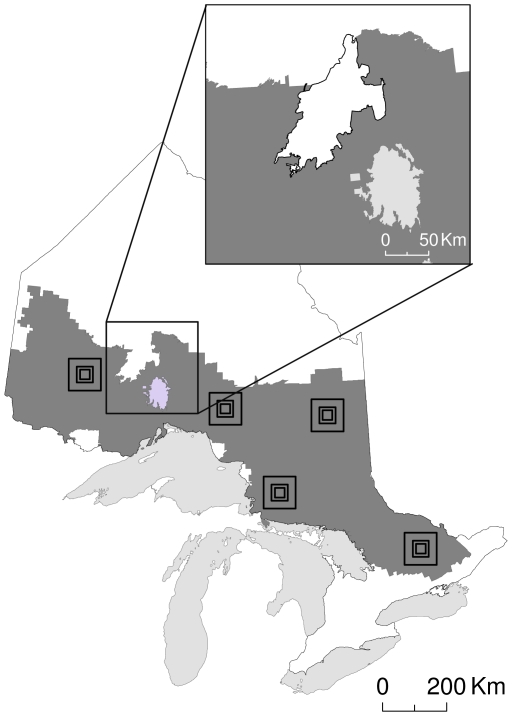
- The authors used circuit theory via CIRCUITSCAPE 3.5 on a forest resource inventory map of Ontario, Canada, reclassified for American marten (*Martes americana*) habitat quality from 1 (low) to 3 (high).
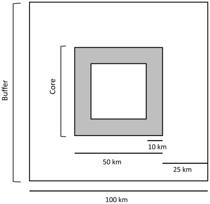
- They used 5 replicate 10,000-km² plots, each with a 2,500-km² core and a 25-km buffer; pixels were 0.0625 km² (160,000 pixels per plot). They estimated resistance between source and destination sites 10 km apart, with 10 random pairs in each inner and outer core per plot (n = 100 pairs), then pooled data over plots for comparisons (n = 50).
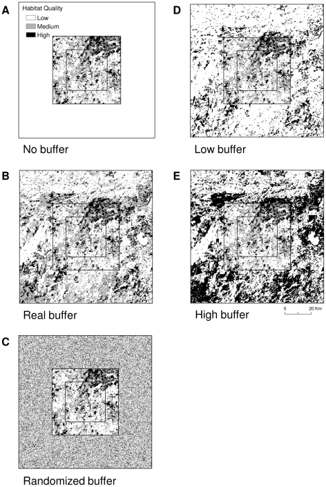
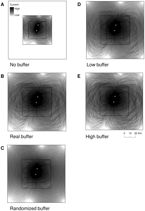
- They compared five scenarios—no buffer, real buffer, randomized buffer, low-biased buffer, and high-biased buffer—using Cohen’s d for paired comparisons, interpreting d = 0.2 as small, 0.5 as medium, and 0.8 as large.
Limitations
- Stated in the paper: the results are based on a relatively simple plot design with a direct path between sites and no barriers or narrow habitat passages; artificial boundaries may have a greater effect in more complex landscapes.
- Stated in the paper: buffer width and composition are project-specific and may be arbitrary when habitat quality beyond the map is unknown; Circuitscape memory limitations may restrict grids larger than six million cells.
- Stated in the paper: future work is needed on the sensitivity of circuit theory to varying levels of landscape connectivity; the study used simulated data and effect sizes rather than test statistics.
Model-written summary. Check it against the paper before relying on it.
Integrity signals
Registry
Cites
Statistics
Figures
Verification
Claims the paper makes
8 Own interpretation · 6 Own result · 2 No full text of the sources · 1 No basis given
A result the paper reports from its own data — it cites no other source for it, so there is none to check. The quote shows it is in the paper.
In the paper
“When we used the randomized buffer however, resistance estimates were not different than estimates using a buffer of real data for sites in either the inner (d = 0.13) or outer (d = 0.002) cores, as indicated by small effect sizes (Table 2).”
§ The Effect of Map Boundary on Estimates of Landscape Resistance to Animal Movement > Results
plain- Asserted: passes — The authors put it forward as true.
- Checkable: passes — It can be checked against evidence.
- Load-bearing: passes — The paper’s conclusions depend on it.
- Based: passes — The paper gives a reason why it holds.
A result the paper reports from its own data — it cites no other source for it, so there is none to check. The quote shows it is in the paper.
In the paper
“We found no difference in resistance however, between scenarios with a buffer of randomized data and a buffer biased towards high quality, for sites in both the inner (d = 0.15) and outer (d = 0.23) cores, as indicated by small effect sizes (Table 2).”
§ The Effect of Map Boundary on Estimates of Landscape Resistance to Animal Movement > Results
plain- Asserted: passes — The authors put it forward as true.
- Checkable: passes — It can be checked against evidence.
- Load-bearing: passes — The paper’s conclusions depend on it.
- Based: passes — The paper gives a reason why it holds.
A result the paper reports from its own data — it cites no other source for it, so there is none to check. The quote shows it is in the paper.
In the paper
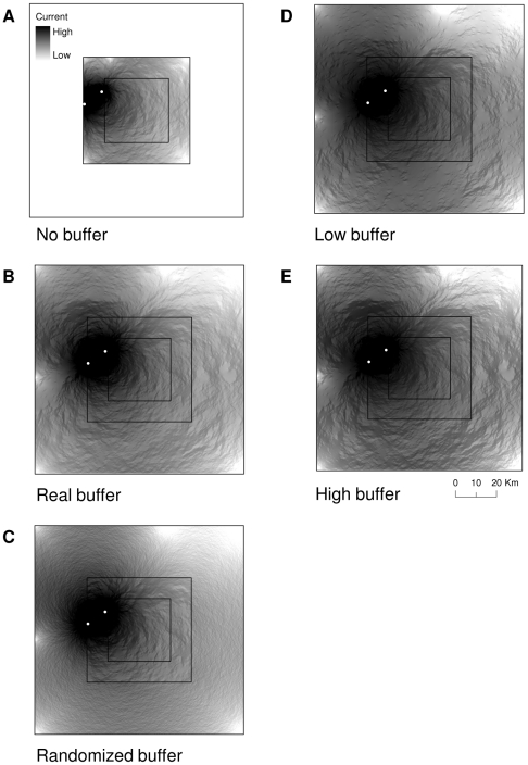
“Resistance was overestimated in the scenario with no buffer relative to the buffer of real data (Figures 4–5) for sites in both the inner (d = 1.50) and outer (d = 0.90) cores, as indicated by large effect sizes (Table 2).”
§ The Effect of Map Boundary on Estimates of Landscape Resistance to Animal Movement > Results
plaindirect- Asserted: passes — The authors put it forward as true.
- Checkable: passes — It can be checked against evidence.
- Load-bearing: passes — The paper’s conclusions depend on it.
- Based: passes — The paper gives a reason why it holds.
A result the paper reports from its own data — it cites no other source for it, so there is none to check. The quote shows it is in the paper.
In the paper
“We found that the scenario with no buffer overestimated resistance relative to when we biased the real buffer toward high habitat quality, for both the inner (d = 0.90) and outer (d = 0.90) cores (Table 2).”
§ The Effect of Map Boundary on Estimates of Landscape Resistance to Animal Movement > Results
plaindirect- Asserted: passes — The authors put it forward as true.
- Checkable: passes — It can be checked against evidence.
- Load-bearing: passes — The paper’s conclusions depend on it.
- Based: passes — The paper gives a reason why it holds.
A result the paper reports from its own data — it cites no other source for it, so there is none to check. The quote shows it is in the paper.
In the paper
“Resistance was again overestimated for the scenario with no buffer relative to the buffer biased towards low quality for sites in both the inner (d = 0.75) and outer (d = 0.84) cores (Table 2).”
§ The Effect of Map Boundary on Estimates of Landscape Resistance to Animal Movement > Results
plaindirectn = 50- Asserted: passes — The authors put it forward as true.
- Checkable: passes — It can be checked against evidence.
- Load-bearing: passes — The paper’s conclusions depend on it.
- Based: passes — The paper gives a reason why it holds.
A result the paper reports from its own data — it cites no other source for it, so there is none to check. The quote shows it is in the paper.
In the paper
“Conversely, when we used the randomized buffer, effect sizes were small; resistance did not differ from the buffer with low-biased data for sites in the inner (d = 0.28) or outer (d = 0.37) cores (Table 2).”
§ The Effect of Map Boundary on Estimates of Landscape Resistance to Animal Movement > Results
plainn = 50- Asserted: passes — The authors put it forward as true.
- Checkable: passes — It can be checked against evidence.
- Load-bearing: passes — The paper’s conclusions depend on it.
- Based: passes — The paper gives a reason why it holds.
A conclusion the paper draws from its own results — it cites no other source for it, so there is none to check. The quote shows it is in the paper.
In the paper
“This feature, however, leads to a potential problem; artificial boundaries may act as barriers to dispersal for the model organisms (random walkers) when, in reality, habitat beyond the boundary is available for use by real organisms.”
§ The Effect of Map Boundary on Estimates of Landscape Resistance to Animal Movement > Introduction
hedgedconditional- Asserted: passes — The authors put it forward as true.
- Checkable: passes — It can be checked against evidence.
- Load-bearing: passes — The paper’s conclusions depend on it.
- Based: passes — The paper gives a reason why it holds.
A conclusion the paper draws from its own results — it cites no other source for it, so there is none to check. The quote shows it is in the paper.
In the paper
“As predicted, resistance was overestimated on maps with artificial boundaries, and the addition of a buffer removed the bias.”
- Also stated in: § Discussion · plain
“A buffer around the artificial boundary removed the barrier to movement and produced a more accurate estimate of resistance.”
§ The Effect of Map Boundary on Estimates of Landscape Resistance to Animal Movement > Discussion
plaindirect- Asserted: passes — The authors put it forward as true.
- Checkable: passes — It can be checked against evidence.
- Load-bearing: passes — The paper’s conclusions depend on it.
- Based: passes — The paper gives a reason why it holds.
- Also stated in: § Discussion · plain
A conclusion the paper draws from its own results — it cites no other source for it, so there is none to check. The quote shows it is in the paper.
In the paper
“Artificial boundaries on maps biased landscape resistance estimated with circuit theory.”
- Also stated in: § Conclusions/Significance · plain
“Artificial map boundaries overestimate resistance values.”
§ The Effect of Map Boundary on Estimates of Landscape Resistance to Animal Movement > Discussion
plaindirect- Asserted: passes — The authors put it forward as true.
- Checkable: passes — It can be checked against evidence.
- Load-bearing: passes — The paper’s conclusions depend on it.
- Based: passes — The paper gives a reason why it holds.
- Rests on an assumption: The outcome of the simulation is not species or landscape specific.
- Also stated in: § Conclusions/Significance · plain
A conclusion the paper draws from its own results — it cites no other source for it, so there is none to check. The quote shows it is in the paper.
In the paper
“As such, the randomized buffer that we used was more appropriate than a buffer based on satellite imagery because we could not infer habitat suitability for martens otherwise.”
§ The Effect of Map Boundary on Estimates of Landscape Resistance to Animal Movement > Discussion
plaindirect- Asserted: passes — The authors put it forward as true.
- Checkable: passes — It can be checked against evidence.
- Load-bearing: passes — The paper’s conclusions depend on it.
- Based: passes — The paper gives a reason why it holds.
- It may state two separate claims as one. 3
- Probably not a substantial claim. 2
A conclusion the paper draws from its own results — it cites no other source for it, so there is none to check. The quote shows it is in the paper.
In the paper
“A buffer around the artificial boundary removed the barrier to movement and produced a more accurate estimate of resistance.”
§ The Effect of Map Boundary on Estimates of Landscape Resistance to Animal Movement > Discussion
plaindirect- Asserted: passes — The authors put it forward as true.
- Checkable: passes — It can be checked against evidence.
- Load-bearing: passes — The paper’s conclusions depend on it.
- Based: passes — The paper gives a reason why it holds.
It may state two separate claims as one.
The paper states this without a source or data behind it here, so there is nothing to check it against. The quote shows it is in the paper.
In the paper
“Artificial boundaries of a map, boundaries that exist on the land-cover map but not on the ground, will arise in studies that span large areas where compatible remotely-sensed land-cover data might not exist for the entire region of interest.”
§ The Effect of Map Boundary on Estimates of Landscape Resistance to Animal Movement > Introduction
hedgeddirect- Asserted: passes — The authors put it forward as true.
- Checkable: passes — It can be checked against evidence.
- Load-bearing: passes — The paper’s conclusions depend on it.
- Based: passes — The paper gives a reason why it holds.
Probably not a substantial claim.
A claim is checked only against the cited paper’s full text, never its abstract, and none is available for its sources.
In the paper
“One of the reasons circuit theory is appealing as a model of gene flow and individual movement is that the incorporation of random walkers on networks to estimate landscape resistance allows resistance to decrease with increasing connectivity, path width, and path redundancy [11], [14].”
§ The Effect of Map Boundary on Estimates of Landscape Resistance to Animal Movement > Introduction
What the sources say
plain- Asserted: passes — The authors put it forward as true.
- Checkable: passes — It can be checked against evidence.
- Load-bearing: fails — The paper’s conclusions may not depend on it.
- Based: passes — The paper gives a reason why it holds.
Probably not a substantial claim. The paper’s conclusions may not depend on it.
A conclusion the paper draws from its own results — it cites no other source for it, so there is none to check. The quote shows it is in the paper.
In the paper
“This is because artificial boundaries limit the space available to random walkers, which artificially reduces the number of paths to each node, thus increasing perceived resistance.”
§ The Effect of Map Boundary on Estimates of Landscape Resistance to Animal Movement > Discussion
plaindirect- Asserted: passes — The authors put it forward as true.
- Checkable: passes — It can be checked against evidence.
- Load-bearing: passes — The paper’s conclusions depend on it.
- Based: passes — The paper gives a reason why it holds.
It may state two separate claims as one.
A claim is checked only against the cited paper’s full text, never its abstract, and none is available for its sources.
In the paper
“Several authors have alluded to the idea that artificial boundaries might influence the results of least cost path and landscape resistance models [2], [11], [15]–[18], but to our knowledge, no one has directly addressed the issue.”
§ The Effect of Map Boundary on Estimates of Landscape Resistance to Animal Movement > Introduction
What the sources say
- Not checked — no full text of the sourcecites [2] P Beier, 2008, Forks in the road: Choices in procedures for designing wildland linkages., Conserv Biol source
- Not checked — no full text of the sourcecites [11] BH McRae, 2008, Using circtuit theory to model connectivity in ecology, evolution, and conservation., Ecology source
- Not checked — no full text of the sourcecites [15] F Adriaensen, 2003, The application of ‘least-cost’ modelling as a functional landscape model., Landscape Urban Plan source
- Not checked — no full text of the sourcecites [16] G Verbeylen, 2003, Does matrix resistance influence red squirrel (Sciurus vulgaris L. 1758) distribution in an urban landscape?, Landscape Ecol source
- Not checked — no full text of the sourcecites [17] L Pascual-Hortal, 2007, Impact of spatial scale on the identification of critical habitat patches for the maintenance of landscape connectivity., Landscape Urban Plan source
- Not checked — no full text of the sourcecites [18] JA Lee-Yaw, 2009, Do landscape processes predict phylogeographic patterns in the wood frog?, Mol Ecol source
hedged- Asserted: passes — The authors put it forward as true.
- Checkable: passes — It can be checked against evidence.
- Load-bearing: passes — The paper’s conclusions depend on it.
- Based: passes — The paper gives a reason why it holds.
It may state two separate claims as one.
The paper relies on this without support.
The outcome of the simulation is not species or landscape specific.
“The species of interest and area of study that we used for our simulation is irrelevant however, as we did not expect the outcome to be either species or landscape specific.”
The authors state this as an assumption.
The true habitat composition beyond the map boundaries is unknown.
“This buffer was a substitute for the true data in scenario 2 (assuming the true data were unknown).”
Claims other papers make about this one
Each is checked against this paper’s own text: does it say what the citing paper says it does?
The cited source says what the claim attributes to it.
In the citing paper
“To minimize border effects that could be formed by the tiling process [51], we created a buffer around each tile with the surrounding land cover data to form larger and overlapping calculation areas for processing in Circuitscape (Figure 2).”
From Applying circuit theory for corridor expansion and management at regional scales: tiling, pinch points, and omnidirectional connectivity (2014) · cites this paper as [51]
Citations
Cites
USING CIRCUIT THEORY TO MODEL CONNECTIVITY IN ECOLOGY, EVOLUTION, AND CONSERVATION
McRae, B. H., Dickson, B. G., Keitt, T. H., & Shah, V. B. (2008) · Ecology · doi:10.1890/07-1861.1 · Cited by 2,244
The application of ‘least-cost’ modelling as a functional landscape model
Adriaensen, F., Chardon, J. P., De Blust, G., Swinnen, E., Villalba, S., Gulinck, H., & Matthysen, E. (2003) · Landscape and Urban Planning · doi:10.1016/s0169-2046(02)00242-6 · Cited by 1,342
McRae, B. H. (2006) · Evolution · doi:10.1111/j.0014-3820.2006.tb00500.x · Cited by 1,081
Circuit theory predicts gene flow in plant and animal populations
McRae, B. H., & Beier, P. (2007) · Proceedings of the National Academy of Sciences · doi:10.1073/pnas.0706568104 · Cited by 945
McRae, B. H. (2006) · Evolution · doi:10.1554/05-321.1 · Cited by 900
Graph models of habitat mosaics
Urban, D. L., Minor, E. S., Treml, E. A., & Schick, R. S. (2009) · Ecology Letters · doi:10.1111/j.1461-0248.2008.01271.x · Cited by 539
Forks in the Road: Choices in Procedures for Designing Wildland Linkages
BEIER, P., MAJKA, D. R., & SPENCER, W. D. (2008) · Conservation Biology · doi:10.1111/j.1523-1739.2008.00942.x · Cited by 489
Haddad, N. M., Bowne, D. R., Cunningham, A., Danielson, B. J., Levey, D. J., Sargent, S., & Spira, T. (2003) · Ecology · doi:10.1890/0012-9658(2003)084[0609:cubdt]2.0.co;2 · Cited by 475
Designing Large‐Scale Conservation Corridors for Pattern and Process
Rouget, M., Cowling, R. M., Lombard, A. T., Knight, A. T., & Kerley, G. I. H. (2006) · Conservation Biology · doi:10.1111/j.1523-1739.2006.00297.x · Cited by 305
Use of Empirically Derived Source‐Destination Models to Map Regional Conservation Corridors
Cushman, S. A., McKelvey, K. S., & Schwartz, M. K. (2008) · Conservation Biology · doi:10.1111/j.1523-1739.2008.01111.x · Cited by 269
Research works printed but not linked: 1
- J Cohen, 1988, Statistical power analysis for the behavioral sciences, 2nd edition.
Cited by
Sorted by citations
Estimating landscape resistance to movement: a review
Zeller, K. A., McGarigal, K., & Whiteley, A. R. (2012) · Landscape Ecology · doi:10.1007/s10980-012-9737-0 · Cited by 1,007
Landscape connectivity for wildlife: development and validation of multispecies linkage maps
Koen, E. L., Bowman, J., Sadowski, C., & Walpole, A. A. (2014) · Methods in Ecology and Evolution · doi:10.1111/2041-210x.12197 · Cited by 293
Self-citationGene Flow of a Forest-Dependent Bird across a Fragmented Landscape
Adams, R. V., & Burg, T. M. (2015) · PLoS ONE · doi:10.1371/journal.pone.0140938 · Cited by 247
Howey, M. C. L. (2011) · Journal of Archaeological Science · doi:10.1016/j.jas.2011.03.024 · Cited by 168
Pelletier, D., Clark, M., Anderson, M. G., Rayfield, B., Wulder, M. A., & Cardille, J. A. (2014) · PLOS One · doi:10.1371/journal.pone.0084135 · Cited by 158
Metadata
- Authors
- Koen, E. L., Garroway, C. J., Wilson, P. J., & Bowman, J.
- Affiliations
- Trent University (CA)
- Ministry of Natural Resources and Forestry (CA)
- Corresponding author
- Koen, Erin L.
- Venue
- PLoS ONE
- Publisher
- Public Library of Science (PLoS)
- Published
- 2010-07-26
- Volume
- 5
- Issue
- 7
- Pages
- e11785
- ISSN
- 1932-6203 (ISSN-L)
- PMC
- PMC2909918
- OpenAlex
- W2167189097
- Cited by
- 148
- References
- 23
- Citations by year
- 2026: 7 · 2025: 13 · 2024: 8 · 2023: 18 · 2022: 9 · 2021: 9 · 2020: 13 · 2019: 7 · 2018: 6 · 2017: 17 · 2016: 10 · 2015: 11 · 2014: 6 · 2013: 5 · 2012: 5
- FWCI
- 3.72
- Type
- journal article
- Language
- en
- Open access
- gold
- doi.org
- Locations
- PLoS ONE (publishedVersion, cc-by)
- PubMed Central (publishedVersion, cc-by)
- PubMed (publishedVersion)
- RePEc: Research Papers in Economics (submittedVersion)
- DOAJ (DOAJ: Directory of Open Access Journals) (submittedVersion, cc-by-sa)
- Funders
- Natural Sciences and Engineering Research Council of Canada
- Topics
- Physical Sciences › Environmental Science › Ecology › Wildlife-Road Interactions and Conservation
- Physical Sciences › Environmental Science › Ecology › Wildlife Ecology and Conservation
- Physical Sciences › Environmental Science › Ecological Modeling › Species Distribution and Climate Change
- Keywords
- circuit theory, Circuitscape, gene flow, animal dispersal, buffer zones, habitat quality, landscape connectivity, landscape genetics
- MeSH terms
- Animals, Canada, Geography, Models, Theoretical, Ontario, Ecosystem
About these checks
Registry, retraction, Cites and statistics results are computed, not judged, with one exception: a printed reference that no index lists is read once by a model before it counts as a citation error. Claims are extracted by a model and kept only when their quote appears verbatim in the text; each cited source is then checked, with a model’s help, for whether it says what the claim relies on. Those verdicts can be wrong — read the claim’s quote and the cited source before relying on one.
A language model drew the claims from the paper on 2026-11-09, under version 3 of the claim definition (model deepseek-v4.1-flash, prompt extract-v3).
A second model labelled each claim on 2026-11-09 (model jev-1.13-20260917, definition revision gold-guideline-v0.2).
Statistics and arithmetic are recomputed, not judged.
Confidence bands are shown only for fields calibrated on our annotated test set. None is calibrated yet, so no band is shown.
What counts as a claim ›How we measure confidence ›How we check this ›
Are you an author, or do you see a problem with this page? Request a review
