Student or educator? Sign up with your school email and get 6 months of Pro free.
CoChat

The DOI matches its Crossref record; 30 of the 30 references it cites were found in a registry or an index.

Efficient magic state factories with a catalyzed | C C Z ⟩ to 2 | T ⟩ transformation

Open access
Gidney, Craig, Fowler, Austin G. · 2019 · Quantum

Abstract

We present magic state factory constructions for producing | C C Z ⟩ states and | T ⟩ states. For the | C C Z ⟩ factory we apply the surface code lattice surgery construction techniques described in \cite{fowler2018} to the fault-tolerant Toffoli \cite{jones2013, eastin2013distilling}. The resulting factory has a footprint of 12 d × 6 d (where d is the code distance) and produces one | C C Z ⟩ every 5.5 d surface code cycles. Our | T ⟩ state factory uses the | C C Z ⟩ factory's output and a catalyst | T ⟩ state to exactly transform one | C C Z ⟩ state into two | T ⟩ states. It has a footprint 25 % smaller than the factory in \cite{fowler2018} but outputs | T ⟩ states twice as quickly. We show how to generalize the catalyzed transformation to arbitrary phase angles, and note that the case θ = 22.5 ∘ produces a particularly efficient circuit for producing | T ⟩ states. Compared to using the 12 d × 8 d × 6.5 d | T ⟩ factory of \cite{fowler2018}, our | C C Z ⟩ factory can quintuple the speed of algorithms that are dominated by the cost of applying Toffoli gates, including Shor's algorithm \cite{shor1994} and the chemistry algorithm of Babbush et al. \cite{babbush2018}. Assuming a physical gate error rate of 10 − 3 , our CCZ factory can produce ∼ 10 10 states on average before an error occurs. This is sufficient for classically intractable instantiations of the chemistry algorithm, but for more demanding algorithms such as Shor's algorithm the mean number of states until failure can be increased to ∼ 10 12 by increasing the factory footprint ∼ 20 % .

Overview

The claims and statistics of this paper haven’t been checked yet.

Free: it reads the open-access text and checks the first 5 claims that cite a source we can check. Create a free account to check every claim.

A few free checks a day · papers already verified open instantly · results are public

Integrity signals

Registry

Crossref · 10.22331/q-2019-04-30-135

Cites

30 of 30 references verified0 citation errors · 0 not checkable

Statistics

Figures

Image 1
CC-BY · From the PDF
Image 2
CC-BY · From the PDF
Figure 4 Comparison of the to-scale diagram style from [15] with the exaggerated-spacing diagram style used by this paper. The to-scale diagram style emphasizes how things fit together and is ideal when reasoning geometrically. The exaggerated-spacing diagram style emphasize how things connect together and is ideal when reasoning topologically. An even more abstract diagram style for lattice surgery is the ZX calculus [10]. In Figure 9 we show how translate a topological diagram into a ZX calculus graph.
Figure 4 Comparison of the to-scale diagram style from [15] with the exaggerated-spacing diagram style used by this paper. The to-scale diagram style emphasizes how things fit together and is ideal when reasoning geometrically. The exaggerated-spacing diagram style emphasize how things connect together and is ideal when reasoning topologically. An even more abstract diagram style for lattice surgery is the ZX calculus [10]. In Figure 9 we show how translate a topological diagram into a ZX calculus graph.CC-BY · From the PDF
Figure 5 Quantum circuit for the 8 | T 〉 28 ϵ 2 → | CCZ 〉 factory. A rewrite of figure 3 from [21]. The box with blue circles in the top right is a state display from the online simulator Quirk, with each circle representing an amplitude (the radius of the colored circle indicates the amplitude's magnitude, and the angle of the line rooted at the center of the circle indicates the phase). The state display is showing that the output state is a | CCZ 〉 state. The small circled pluses in the circuit are X-axis controls (equivalent to a normal control surrounded by Hadamard gates); whenever one of these controls directly precedes a measurement the measurement corresponds to a Pauli product measurement. The post-selection operation represents the classical control software determining if the an error was detected; if it fails the output must be discarded. Pauli operations and classically-controlled Pauli operations appear here, but not in Figure 8, because they are performed entirely within classical control software. The circuit can be opened in Quirk by following this link. Discerning readers can follow the link and edit the circuit in order to confirm that adding a single Z error by any T gate is caught by the post-selection, and also that all possible pairs of Z errors escape detection.
Figure 5 Quantum circuit for the 8 | T 〉 28 ϵ 2 → | CCZ 〉 factory. A rewrite of figure 3 from [21]. The box with blue circles in the top right is a state display from the online simulator Quirk, with each circle representing an amplitude (the radius of the colored circle indicates the amplitude's magnitude, and the angle of the line rooted at the center of the circle indicates the phase). The state display is showing that the output state is a | CCZ 〉 state. The small circled pluses in the circuit are X-axis controls (equivalent to a normal control surrounded by Hadamard gates); whenever one of these controls directly precedes a measurement the measurement corresponds to a Pauli product measurement. The post-selection operation represents the classical control software determining if the an error was detected; if it fails the output must be discarded. Pauli operations and classically-controlled Pauli operations appear here, but not in Figure 8, because they are performed entirely within classical control software. The circuit can be opened in Quirk by following this link. Discerning readers can follow the link and edit the circuit in order to confirm that adding a single Z error by any T gate is caught by the post-selection, and also that all possible pairs of Z errors escape detection.CC-BY · From the PDF
Figure 6 Time slices of lattice surgery activity during production of a single | CCZ 〉 state. Each red square corresponds to a qubit, and the label inside the red square identifies the qubit from Figure 5 that the square corresponds to. Gray rectangles correspond to X stabilizer measurements between sets of qubits. The red arrows labelled 'T' correspond to a noisy T state entering the system. It is possible to double the throughput shown here by interleaving the production of two states (shown in Figure 7).
Figure 6 Time slices of lattice surgery activity during production of a single | CCZ 〉 state. Each red square corresponds to a qubit, and the label inside the red square identifies the qubit from Figure 5 that the square corresponds to. Gray rectangles correspond to X stabilizer measurements between sets of qubits. The red arrows labelled 'T' correspond to a noisy T state entering the system. It is possible to double the throughput shown here by interleaving the production of two states (shown in Figure 7).CC-BY · From the PDF
Figure 7 Time slices of lattice surgery activity during production of | CCZ 〉 states by the 8 | T 〉 28 ϵ 2 → | CCZ 〉 factory. To maximize utilization, two states are produced concurrently. Each red or blue square corresponds to a qubit, and the label inside the square identifies the qubit from Figure 5 that the square corresponds to. Gray rectangles correspond to X stabilizer measurements between sets of qubits. The red arrows labelled 'T' correspond to a noisy T state entering the system. Blue squares correspond to qubits involved in producing one of the states, and red squares correspond to qubits involved in producing the other state. The red squares in each step are exactly identical to the red squares shown in the matching step of Figure 6. See Figure 8 for a 3D topological diagram corresponding to the time slices.
Figure 7 Time slices of lattice surgery activity during production of | CCZ 〉 states by the 8 | T 〉 28 ϵ 2 → | CCZ 〉 factory. To maximize utilization, two states are produced concurrently. Each red or blue square corresponds to a qubit, and the label inside the square identifies the qubit from Figure 5 that the square corresponds to. Gray rectangles correspond to X stabilizer measurements between sets of qubits. The red arrows labelled 'T' correspond to a noisy T state entering the system. Blue squares correspond to qubits involved in producing one of the states, and red squares correspond to qubits involved in producing the other state. The red squares in each step are exactly identical to the red squares shown in the matching step of Figure 6. See Figure 8 for a 3D topological diagram corresponding to the time slices.CC-BY · From the PDF
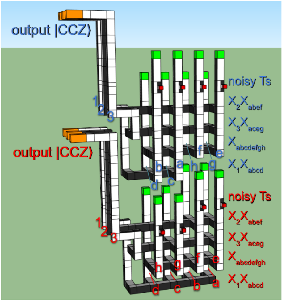
Figure 8 3D topological diagram for our construction of the 8 | T 〉 28 ϵ 2 → | CCZ 〉 factory. The spacing between qubits has been increased to make it possible to see the internal structure. White (black) surfaces correspond to boundaries where chains of Z (X) errors can terminate. Corresponds to the time slices from Figure 7. Time increases from bottom to top. The vertical poles correspond to qubits from Figure 5. Red boxes indicate connection points for noisy | T 1 〉 states produced by a level 1 T factory. The green boxes atop the columns are performing either an X or Y basis measurement at half code distance, as described in [15], by including or omitting an S gate performed using twists [6]. Using half code distance is acceptable because, at the location in the factory where these operations are performed (i.e. after the T injections), individual errors are detected as distillation failures. The labels along the right hand side indicate the stabilizer measurements occurring at each time. The red/blue coloring of labels matches the red/blue coloring of Figure 7. Note that inserting the | T 1 〉 state has a depth of 1.5, unlike the other steps which have depth 1. Each horizontal bar linking several vertical poles is a stabilizer measurement of a product of logical X observables. The groups of three qubits highlighted orange and exiting left are the | CCZ 〉 states being output (note that the middle pole of each | CCZ 〉 state is rotated with respect to the others, with white on top instead of black on top). The two instances of the factory that are shown differ slightly. Their qubits have been permuted so that each factory's top layer fits into a void at the bottom of the following factory, saving a layer of depth.
Figure 8 3D topological diagram for our construction of the 8 | T 〉 28 ϵ 2 → | CCZ 〉 factory. The spacing between qubits has been increased to make it possible to see the internal structure. White (black) surfaces correspond to boundaries where chains of Z (X) errors can terminate. Corresponds to the time slices from Figure 7. Time increases from bottom to top. The vertical poles correspond to qubits from Figure 5. Red boxes indicate connection points for noisy | T 1 〉 states produced by a level 1 T factory. The green boxes atop the columns are performing either an X or Y basis measurement at half code distance, as described in [15], by including or omitting an S gate performed using twists [6]. Using half code distance is acceptable because, at the location in the factory where these operations are performed (i.e. after the T injections), individual errors are detected as distillation failures. The labels along the right hand side indicate the stabilizer measurements occurring at each time. The red/blue coloring of labels matches the red/blue coloring of Figure 7. Note that inserting the | T 1 〉 state has a depth of 1.5, unlike the other steps which have depth 1. Each horizontal bar linking several vertical poles is a stabilizer measurement of a product of logical X observables. The groups of three qubits highlighted orange and exiting left are the | CCZ 〉 states being output (note that the middle pole of each | CCZ 〉 state is rotated with respect to the others, with white on top instead of black on top). The two instances of the factory that are shown differ slightly. Their qubits have been permuted so that each factory's top layer fits into a void at the bottom of the following factory, saving a layer of depth.CC-BY · From the PDF
Figure 9 A substitution procedure (left) for translating our 3D topological diagrams into (nearly) the ZX calculus [10], as well as an example translation of one of the CCZ factories from Figure 8 (right). We use black (white) nodes instead of green (red) nodes (the usual notation for the ZX calculus) so that the node colors match the boundary colors in the 3D topological diagrams. Pieces with two ports are translated into edges or degree-2 nodes of either color. Pieces with three or more ports are translated into a node of matching color. The Z ⊗ Z measurement of a qubit vs a | T 〉 state followed by measuring the qubit in the X or Y basis depending on the outcome of the parity measurement is translated into a (non-standard) red node. The red node can be expanded into a proper ZX calculus construction, but we do not attempt to do so. The ZX calculus graph is more amenable to verification than the 3D diagram. The reverse translation, from ZX calculus graph to 3D topological diagram, is often more difficult.
Figure 9 A substitution procedure (left) for translating our 3D topological diagrams into (nearly) the ZX calculus [10], as well as an example translation of one of the CCZ factories from Figure 8 (right). We use black (white) nodes instead of green (red) nodes (the usual notation for the ZX calculus) so that the node colors match the boundary colors in the 3D topological diagrams. Pieces with two ports are translated into edges or degree-2 nodes of either color. Pieces with three or more ports are translated into a node of matching color. The Z ⊗ Z measurement of a qubit vs a | T 〉 state followed by measuring the qubit in the X or Y basis depending on the outcome of the parity measurement is translated into a (non-standard) red node. The red node can be expanded into a proper ZX calculus construction, but we do not attempt to do so. The ZX calculus graph is more amenable to verification than the 3D diagram. The reverse translation, from ZX calculus graph to 3D topological diagram, is often more difficult.CC-BY · From the PDF
Figure 10 A circuit that transforms a | CCZ 〉 state into three | T 〉 states by applying Clifford operations and a single T gate. By using one of the outputs to fuel the next iteration, the circuit can be re-interpreted as a circuit that turns one | CCZ 〉 into two | T 〉 states when catalyzed by one | T 〉 state. The boxes with blue circles are state displays from the online simulator Quirk, with each circle representing an amplitude (the radius of the colored circle indicates the amplitude's magnitude, and the angle of the line rooted at the center of the circle indicates the phase). The state displays are showing that the input state is a | CCZ 〉 and the output states are | T 〉 states. The small circled pluses are X-axis controls (equivalent to a normal control surrounded by Hadamard gates). The circuit can be opened in Quirk by following this link.
Figure 10 A circuit that transforms a | CCZ 〉 state into three | T 〉 states by applying Clifford operations and a single T gate. By using one of the outputs to fuel the next iteration, the circuit can be re-interpreted as a circuit that turns one | CCZ 〉 into two | T 〉 states when catalyzed by one | T 〉 state. The boxes with blue circles are state displays from the online simulator Quirk, with each circle representing an amplitude (the radius of the colored circle indicates the amplitude's magnitude, and the angle of the line rooted at the center of the circle indicates the phase). The state displays are showing that the input state is a | CCZ 〉 and the output states are | T 〉 states. The small circled pluses are X-axis controls (equivalent to a normal control surrounded by Hadamard gates). The circuit can be opened in Quirk by following this link.CC-BY · From the PDF
Figure 11 A circuit for catalyzed | T 〉 state production, specialized for lattice surgery. Given a | CCZ 〉 state (first three qubits) and a | T 〉 state (fourth qubit), produces three | T 〉 states. Red areas correspond to a product-of-Paulis measurement. The blue area happens entirely within classical control software. The S ancilla is preparing an | S 〉 state that can be used to correct the T gate teleportation used to perform the Z -1 / 4 gate from Figure 10. The B ancilla is being used to perform the X -1 / 2 gate from Figure 10. The A ancilla is being used to perform the multi-target CNOT from Figure 10. The boxes with blue circles, at the beginning and end of the circuit, are state displays from the online simulator Quirk. Each circle represents an amplitude (the radius of the colored circle indicates the amplitude's magnitude, and the angle of the line rooted at the center of the circle indicates the phase). The state displays are showing that the input and output states are | CCZ 〉 and | T 〉 states as described. The small circled pluses in the circuit are X-axis controls (equivalent to a normal control surrounded by Hadamard gates); whenever one of these controls directly precedes a measurement the measurement corresponds to a Pauli product measurement. The circuit can be opened in Quirk by following this link.
Figure 11 A circuit for catalyzed | T 〉 state production, specialized for lattice surgery. Given a | CCZ 〉 state (first three qubits) and a | T 〉 state (fourth qubit), produces three | T 〉 states. Red areas correspond to a product-of-Paulis measurement. The blue area happens entirely within classical control software. The S ancilla is preparing an | S 〉 state that can be used to correct the T gate teleportation used to perform the Z -1 / 4 gate from Figure 10. The B ancilla is being used to perform the X -1 / 2 gate from Figure 10. The A ancilla is being used to perform the multi-target CNOT from Figure 10. The boxes with blue circles, at the beginning and end of the circuit, are state displays from the online simulator Quirk. Each circle represents an amplitude (the radius of the colored circle indicates the amplitude's magnitude, and the angle of the line rooted at the center of the circle indicates the phase). The state displays are showing that the input and output states are | CCZ 〉 and | T 〉 states as described. The small circled pluses in the circuit are X-axis controls (equivalent to a normal control surrounded by Hadamard gates); whenever one of these controls directly precedes a measurement the measurement corresponds to a Pauli product measurement. The circuit can be opened in Quirk by following this link.CC-BY · From the PDF
Figure 12 Time slices of lattice surgery activity during transformation of a | CCZ 〉 state (orange qubits labelled 1, 2, 3) into three | T 〉 states (shown in red in last slice), catalyzed by a | T 〉 state (bottom right qubit in red). Black and dark gray bars correspond to stabilizer measurements. Ancillae qubits are shown in blue. The code distance of the ancillae qubits is doubled when single-qubit Clifford operations are being applied, to ensure there is sufficient suppression of errors. The light gray '(CCZ)' box to the left will be used by the CCZ factory producing | CCZ 〉 states to be transformed. See Figure 13 for a 3D topological diagram corresponding to the time slices. Every step being performed can be matched up with a step from Figure 11, and the qubit labels shown here correspond to the qubit labels there.
Figure 12 Time slices of lattice surgery activity during transformation of a | CCZ 〉 state (orange qubits labelled 1, 2, 3) into three | T 〉 states (shown in red in last slice), catalyzed by a | T 〉 state (bottom right qubit in red). Black and dark gray bars correspond to stabilizer measurements. Ancillae qubits are shown in blue. The code distance of the ancillae qubits is doubled when single-qubit Clifford operations are being applied, to ensure there is sufficient suppression of errors. The light gray '(CCZ)' box to the left will be used by the CCZ factory producing | CCZ 〉 states to be transformed. See Figure 13 for a 3D topological diagram corresponding to the time slices. Every step being performed can be matched up with a step from Figure 11, and the qubit labels shown here correspond to the qubit labels there.CC-BY · From the PDF
Figure 13 3D topological diagram of a lattice surgery circuit transforming a | CCZ 〉 state (orange-tipped inputs at bottom) and a | T 〉 state (bottom right red-tipped input) into three | T 〉 states (red-tipped outputs at top). We conservatively assume that the green boxes are large enough to perform any single-qubit Clifford with negligible error. See Figure 8 for details about how to interpret the diagram.
Figure 13 3D topological diagram of a lattice surgery circuit transforming a | CCZ 〉 state (orange-tipped inputs at bottom) and a | T 〉 state (bottom right red-tipped input) into three | T 〉 states (red-tipped outputs at top). We conservatively assume that the green boxes are large enough to perform any single-qubit Clifford with negligible error. See Figure 8 for details about how to interpret the diagram.CC-BY · From the PDF
Figure 14 Generalized phase catalysis circuit. Given a Z θ | + 〉 catalyst, two Z θ operations can be applied via stabilizer gates, one AND computation gate (notation from [17]), and one Z 2 θ gate.
Figure 14 Generalized phase catalysis circuit. Given a Z θ | + 〉 catalyst, two Z θ operations can be applied via stabilizer gates, one AND computation gate (notation from [17]), and one Z 2 θ gate.CC-BY · From the PDF
Figure 15 Using a catalyst | √ T 〉 state to create 2 additional | √ T 〉 states using cheap stabilizer operations, one T gate, and one AND computation. Has a T-cost of 5 [21, 17], implying the T-cost of a √ T state is at most 2 . 5 .
Figure 15 Using a catalyst | √ T 〉 state to create 2 additional | √ T 〉 states using cheap stabilizer operations, one T gate, and one AND computation. Has a T-cost of 5 [21, 17], implying the T-cost of a √ T state is at most 2 . 5 .CC-BY · From the PDF
Figure 16 3D topological diagram of a re-arrangement of the level 1 T factory from [15]. Quantities are quoted in units of d/ 2 instead of d because the factory is performed at half code distance. Improves the depth from 13 d/ 2 to 12 . 5 d/ 2 , increasing the output rate by roughly 4%, which ensures four level 1 T factories is sufficient to feed our T-catalyzed factory. There are two variants of the factory: the one shown with an output on the left (A) and the one shown with an output on the right (B). The qubits of A and B have been permuted so that their first stabilizer measurement involves qubits that are all on the same side, allowing the stabilizer measurement to be performed without using a central bar. The second measurement of B (the first measurement using the central bar) is over the back 8 qubits and the last measurement of A is over the front 8 qubits. This allows B to be lowered by half of d/ 2 , so that B rests on the level 0 | T 〉 injections to the right of A. The transition back from B to A cannot be lowered quite as far, because the top of B would intersect the first central bar used in A. Overall this optimization saves 0 . 5 d/ 2 depth relative to the interleaving technique used in [15].
Figure 16 3D topological diagram of a re-arrangement of the level 1 T factory from [15]. Quantities are quoted in units of d/ 2 instead of d because the factory is performed at half code distance. Improves the depth from 13 d/ 2 to 12 . 5 d/ 2 , increasing the output rate by roughly 4%, which ensures four level 1 T factories is sufficient to feed our T-catalyzed factory. There are two variants of the factory: the one shown with an output on the left (A) and the one shown with an output on the right (B). The qubits of A and B have been permuted so that their first stabilizer measurement involves qubits that are all on the same side, allowing the stabilizer measurement to be performed without using a central bar. The second measurement of B (the first measurement using the central bar) is over the back 8 qubits and the last measurement of A is over the front 8 qubits. This allows B to be lowered by half of d/ 2 , so that B rests on the level 0 | T 〉 injections to the right of A. The transition back from B to A cannot be lowered quite as far, because the top of B would intersect the first central bar used in A. Overall this optimization saves 0 . 5 d/ 2 depth relative to the interleaving technique used in [15].CC-BY · From the PDF
Figure 17 Time slices of activity during catalyzed | T 〉 state distillation. Every step being performed can be matched up with Figure 5 and Figure 12. See Figure 18 for the 3D topological diagram these time slices come from.
Figure 17 Time slices of activity during catalyzed | T 〉 state distillation. Every step being performed can be matched up with Figure 5 and Figure 12. See Figure 18 for the 3D topological diagram these time slices come from.CC-BY · From the PDF
Figure 18 3D topological diagram of the full | T 〉 -catalyzed 8 | T 〉 28 ϵ 2 → 2 | T 〉 factory. Contrast with the time slices from Figure 17, and the circuit in Figure 5 combined with the circuit in Figure 10. Single-qubit Clifford gates that would affect the catalyst | T 〉 if they failed are performed with extremely conservative code distance (large green boxes).
Figure 18 3D topological diagram of the full | T 〉 -catalyzed 8 | T 〉 28 ϵ 2 → 2 | T 〉 factory. Contrast with the time slices from Figure 17, and the circuit in Figure 5 combined with the circuit in Figure 10. Single-qubit Clifford gates that would affect the catalyst | T 〉 if they failed are performed with extremely conservative code distance (large green boxes).CC-BY · From the PDF
Figure 19 3D topological diagram showing tiled operation of our CCZ factory (left) and our catalyzed T factory (right). Includes the half-distance level 1 T factories feeding noisy states into the larger factories.
Figure 19 3D topological diagram showing tiled operation of our CCZ factory (left) and our catalyzed T factory (right). Includes the half-distance level 1 T factories feeding noisy states into the larger factories.CC-BY · From the PDF

Verification

Claims the paper makes

The claims and statistics of this paper haven’t been checked yet.

Free: it reads the open-access text and checks the first 5 claims that cite a source we can check. Create a free account to check every claim.

A few free checks a day · papers already verified open instantly · results are public

Self-check

Percentages, sums and reported differences re-computed from the paper’s own numbers.

The self-check needs the paper’s full text.

Citations

Cites

Show all 24 references

Research works printed but not linked: 2

  1. Niel de Beaudrap and Dominic Horsman. The zx calculus is a language for surface code lattice surgery. arXiv preprint arXiv:1704.08670, 2017. URL https://arxiv.org/abs/1704.08670. · arXiv
  2. Yunseong Nam, Yuan Su, and Dmitri Maslov. Approximate quantum fourier transform with o(n log(n)) t gates. arXiv preprint arXiv:1803.04933, 2018. URL https://arxiv.org/abs/1803.04933. · arXiv

Cited by

See all 216

Metadata

Authors
Gidney, C., & Fowler, A. G.
Affiliations
Google (United States) (US)
Venue
Quantum
Published
2019-04-30
Volume
3
Pages
135
ISSN
2521-327X (ISSN-L)
OpenAlex
W2952708034
Cited by
152
References
24
Citations by year
2026: 23 · 2025: 33 · 2024: 22 · 2023: 13 · 2022: 15 · 2021: 16 · 2020: 18 · 2019: 11
FWCI
6.96
Type
journal article
Language
en
Open access
Locations
  • Quantum (publishedVersion, cc-by)
  • arXiv (Cornell University) (submittedVersion)
  • DOAJ (DOAJ: Directory of Open Access Journals) (submittedVersion, cc-by-sa)
  • arXiv (Cornell University) (cc-by)
Topics
  • Physical Sciences › Computer Science › Artificial Intelligence › Quantum Computing Algorithms and Architecture
  • Physical Sciences › Physics and Astronomy › Atomic and Molecular Physics, and Optics › Quantum Information and Cryptography
  • Physical Sciences › Physics and Astronomy › Atomic and Molecular Physics, and Optics › Quantum many-body systems
Keywords
Toffoli gate, surface code, lattice surgery, fault-tolerant quantum computing, quantum chemistry algorithms, Shor's algorithm

About these checks

Registry, retraction, Cites and statistics results are computed, not judged, with one exception: a printed reference that no index lists is read once by a model before it counts as a citation error. Claims are extracted by a model and kept only when their quote appears verbatim in the text; each cited source is then checked, with a model’s help, for whether it says what the claim relies on. Those verdicts can be wrong — read the claim’s quote and the cited source before relying on one.

Statistics and arithmetic are recomputed, not judged.

Confidence bands are shown only for fields calibrated on our annotated test set. None is calibrated yet, so no band is shown.

What counts as a claim ›How we measure confidence ›How we check this ›

Are you an author, or do you see a problem with this page? Request a review

How to cite

Cite CoChat for the checks on this page, and the paper for its own findings.

This page
CoChat. (2026). Citation check: Efficient magic state factories with a catalyzed | C C Z ⟩ to 2 | T ⟩ transformation. https://app.cochat.ai/papers/10.22331/q-2019-04-30-135
The paper
Gidney, C., & Fowler, A. G. (2019). Efficient magic state factories with a catalyzed | C C Z ⟩ to 2 | T ⟩ transformation. Quantum. https://doi.org/10.22331/q-2019-04-30-135

Data sources

Bibliographic data: Semantic Scholar, OpenAlex, Crossref.

Contains information from the Semantic Scholar Academic Graph Datasets, made available under the ODC Attribution License (ODC-BY 1.0).

Semantic Scholar’s data is described in: Kinney, R., et al. (2023). The Semantic Scholar Open Data Platform. arXiv:2301.10140.