

The DOI matches its Crossref record; 3 of the 3 references it cites were found in a registry or an index.
The BRIDGE HadCM3 family of climate models: HadCM3@Bristol v1.0
Published version of a preprint
Abstract
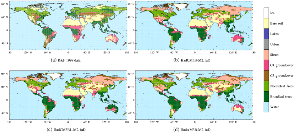
Abstract. Understanding natural and anthropogenic climate change processes involves using computational models that represent the main components of the Earth system: the atmosphere, ocean, sea ice, and land surface. These models have become increasingly computationally expensive as resolution is increased and more complex process representations are included. However, to gain robust insight into how climate may respond to a given forcing, and to meaningfully quantify the associated uncertainty, it is often required to use either or both ensemble approaches and very long integrations. For this reason, more computationally efficient models can be very valuable tools. Here we provide a comprehensive overview of the suite of climate models based around the HadCM3 coupled general circulation model. This model was developed at the UK Met Office and has been heavily used during the last 15 years for a range of future (and past) climate change studies, but has now been largely superseded for many scientific studies by more recently developed models. However, it continues to be extensively used by various institutions, including the BRIDGE (Bristol Research Initiative for the Dynamic Global Environment) research group at the University of Bristol, who have made modest adaptations to the base HadCM3 model over time. These adaptations mean that the original documentation is not entirely representative, and several other relatively undocumented configurations are in use. We therefore describe the key features of a number of configurations of the HadCM3 climate model family, which together make up HadCM3@Bristol version 1.0. In order to differentiate variants that have undergone development at BRIDGE, we have introduced the letter B into the model nomenclature. We include descriptions of the atmosphere-only model (HadAM3B), the coupled model with a low-resolution ocean (HadCM3BL), the high-resolution atmosphere-only model (HadAM3BH), and the regional model (HadRM3B). These also include three versions of the land surface scheme. By comparing with observational datasets, we show that these models produce a good representation of many aspects of the climate system, including the land and sea surface temperatures, precipitation, ocean circulation, and vegetation. This evaluation, combined with the relatively fast computational speed (up to 1000 times faster than some CMIP6 models), motivates continued development and scientific use of the HadCM3B family of coupled climate models, predominantly for quantifying uncertainty and for long multi-millennial-scale simulations.
Overview
The claims and statistics of this paper haven’t been checked yet.
Run the check — free, no account needed. It reads the open-access text and checks the sources it cites.
Integrity signals
Registry
Cites
Statistics
Figures
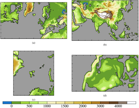
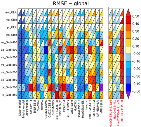
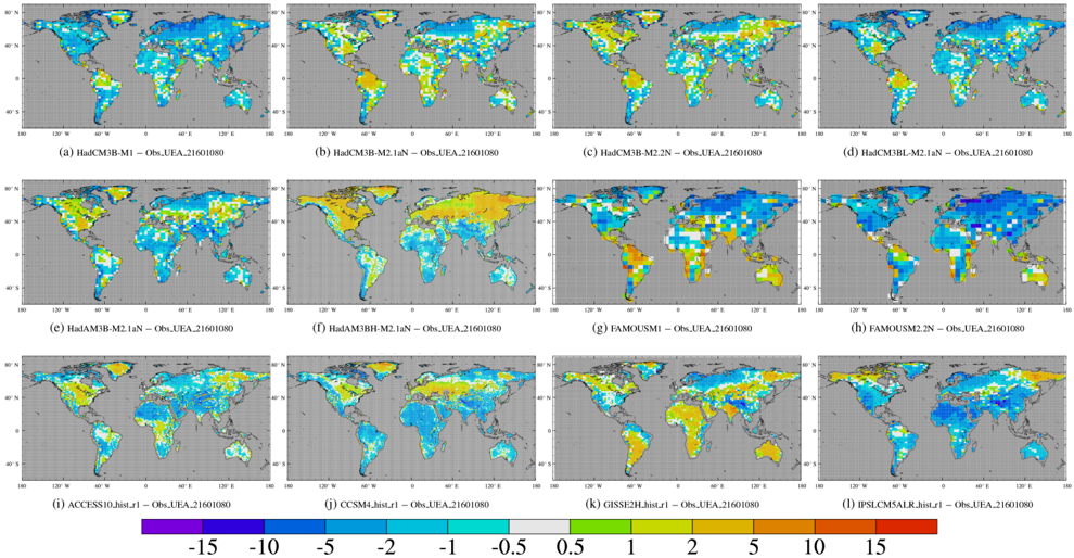
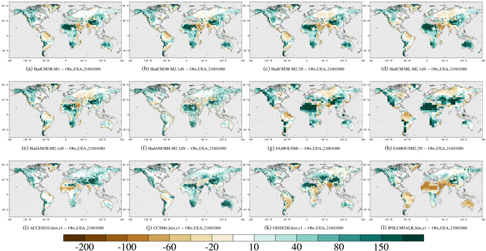
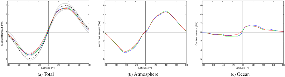
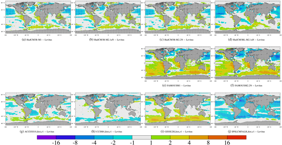
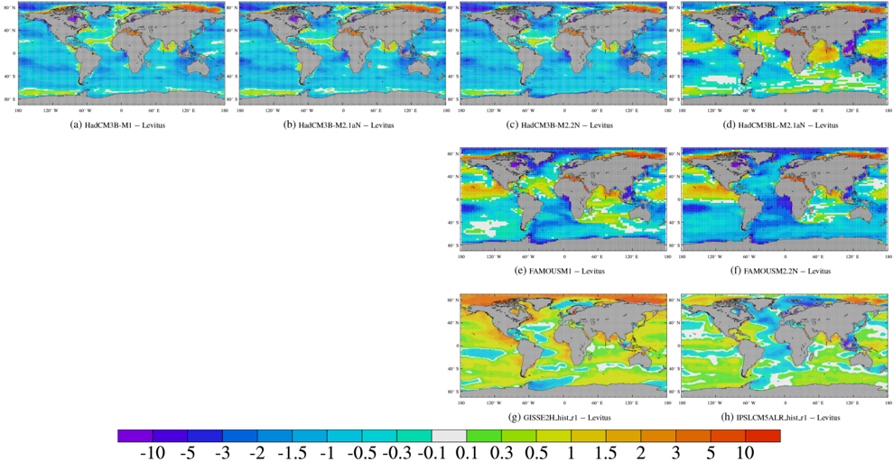
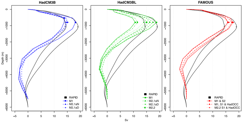
Verification
Claims the paper makes
The claims and statistics of this paper haven’t been checked yet.
Run the check — free, no account needed. It reads the open-access text and checks the sources it cites.
Claims other papers make about this one
Each is checked against this paper’s own text: does it say what the citing paper says it does?
In the citing paper
“HadCM3L has contributed to the Coupled Mode Intercomparison Project experiments demonstrating skill at reproducing the modern-day climate (71, 72) and has been used for an array of different paleoclimate experiments (73–75).”
From Asteroid impact, not volcanism, caused the end-Cretaceous dinosaur extinction (2020) · cites this paper as [71]
Self-check
Percentages, sums and reported differences re-computed from the paper’s own numbers.
The self-check needs the paper’s full text.
Citations
Cites
Eyring, V., Bony, S., Meehl, G. A., Senior, C. A., Stevens, B., Stouffer, R. J., & Taylor, K. E. (2016) · Geoscientific Model Development · doi:10.5194/gmd-9-1937-2016 · Cited by 11,981
Oceanic vertical mixing: A review and a model with a nonlocal boundary layer parameterization
Large, W. G., McWilliams, J. C., & Doney, S. C. (1994) · Reviews of Geophysics · doi:10.1029/94rg01872 · Cited by 4,443
Estimating historical changes in global land cover: Croplands from 1700 to 1992
Ramankutty, N., & Foley, J. A. (1999) · Global Biogeochemical Cycles · doi:10.1029/1999gb900046 · Cited by 2,074
Research works printed but not linked: 113
- Adam, J. C., Clark, E. A., Lettenmaier, D. P., and Wood, E. F.: Correction of Global Precipitation Products for Orographic Effects, J. Climate, 19, 15–38, https://doi.org/10.1175/JCLI3604.1, 2006. · DOI
- Arakawa, A. and Lamb, V. R.: Computational Design of the Basic Dynamical Processes of the UCLA General Circulation Model, in: General Circulation Models of the Atmosphere, edited by: Chang, J., Vol. 17, Methods in Computational Physics: Advances in Research and Applications, 173–265, Elsevier, https://doi.org/10.1016/B978-0-12-460817-7.50009-4, 1977. · DOI
- Armstrong, E., Valdes, P., House, J., and Singarayer, J.: The Role of CO2 and Dynamic Vegetation on the Impact of Temperate Land-Use Change in the HadCM3 Coupled Climate Model, Earth Interact., 20, 1–20, https://doi.org/10.1175/EI-D-15-0036.1, 2016. · DOI
- Arnell, N. W., Hudson, D. A., and Jones, R. G.: Climate change scenarios from a regional climate model: Estimating change in runoff in southern Africa, J. Geophys. Res.-Atmos., 108, 4519, https://doi.org/10.1029/2002JD002782, 2003. · DOI
- Beerling, D. J., Fox, A., Stevenson, D. S., and Valdes, P. J.: Enhanced chemistry-climate feedbacks in past greenhouse worlds, P. Natl. Acad. Sci. USA, 108, 9770–9774, https://doi.org/10.1073/pnas.1102409108, 2011. · DOI · Paper page
- Best, M. J., Pryor, M., Clark, D. B., Rooney, G. G., Essery, R. L. H., Ménard, C. B., Edwards, J. M., Hendry, M. A., Porson, A., Gedney, N., Mercado, L. M., Sitch, S., Blyth, E., Boucher, O., Cox, P. M., Grimmond, C. S. B., and Harding, R. J.: The Joint UK Land Environment Simulator (JULES), model description – Part 1: Energy and water fluxes, Geosci. Model Dev., 4, 677–699, https://doi.org/10.5194/gmd-4-677-2011, 2011. · DOI
- Betts, R. A., Cox, P. M., Collins, M., Harris, P. P., Huntingford, C., and Jones, C. D.: The role of ecosystem-atmosphere interactions in simulated Amazonian precipitation decrease and forest dieback under global climate warming, Theor. Appl. Climatol., 78, 157–175, 2004. · DOI
- Bhaskaran, B., Jones, R. G., Murphy, J. M., and Noguer, M.: Simulations of the Indian summer monsoon using a nested regional climate model: domain size experiments, Clim. Dynam., 12, 573–587, https://doi.org/10.1007/BF00216267, 1996. · DOI
- Booth, B. B. B., Jones, C. D., Collins, M., Totterdell, I. J., Cox, P. M., Sitch, S., Huntingford, C., Betts, R. A., Harris, G. R., and Lloyd, J.: High sensitivity of future global warming to land carbon cycle processes, Environ. Res. Lett., 7, 024002, https://doi.org/10.1088/1748-9326/7/2/024002, 2012. · DOI
- Braconnot, P., Otto-Bliesner, B., Harrison, S., Joussaume, S., Peterchmitt, J.-Y., Abe-Ouchi, A., Crucifix, M., Driesschaert, E., Fichefet, Th., Hewitt, C. D., Kageyama, M., Kitoh, A., Laîné, A., Loutre, M.-F., Marti, O., Merkel, U., Ramstein, G., Valdes, P., Weber, S. L., Yu, Y., and Zhao, Y.: Results of PMIP2 coupled simulations of the Mid-Holocene and Last Glacial Maximum – Part 1: experiments and large-scale features, Clim. Past, 3, 261–277, https://doi.org/10.5194/cp-3-261-2007, 2007. · DOI
- Bradshaw, C. D., Lunt, D. J., Flecker, R., and Davies-Barnard, T.: Disentangling the roles of late Miocene palaeogeography and vegetation – Implications for climate sensitivity, Palaeogeogr. Palaeocl., 417, 17–34, 2015. · DOI
- Bragg, F. J., Lunt, D. J., and Haywood, A. M.: Mid-Pliocene climate modelled using the UK Hadley Centre Model: PlioMIP Experiments 1 and 2, Geosci. Model Dev., 5, 1109–1125, https://doi.org/10.5194/gmd-5-1109-2012, 2012. · DOI
- Bryan, K. and Cox, M. D.: An Approximate Equation of State for Numerical Models of Ocean Circulation, J. Phys. Oceanogr., 2, 510–514, https://doi.org/10.1175/1520-0485(1972)002<0510:AAEOSF>2.0.CO;2, 1972. · DOI
- Clark, D. B., Mercado, L. M., Sitch, S., Jones, C. D., Gedney, N., Best, M. J., Pryor, M., Rooney, G. G., Essery, R. L. H., Blyth, E., Boucher, O., Harding, R. J., Huntingford, C., and Cox, P. M.: The Joint UK Land Environment Simulator (JULES), model description – Part 2: Carbon fluxes and vegetation dynamics, Geosci. Model Dev., 4, 701–722, https://doi.org/10.5194/gmd-4-701-2011, 2011. · DOI
- Claussen, M., Mysak, L., Weaver, A., Crucifix, M., Fichefet, T., Loutre, M.-F., Weber, S., Alcamo, J., Alexeev, V., Berger, A., Calov, R., Ganopolski, A., Goosse, H., Lohmann, G., Lunkeit, F., Mokhov, I., Petoukhov, V., Stone, P., and Wang, Z.: Earth system models of intermediate complexity: closing the gap in the spectrum of climate system models, Clim. Dynam., 18, 579–586, https://doi.org/10.1007/s00382-001-0200-1, 2002. · DOI
- Collins, M., Tett, S. F. B., and Cooper, C.: The internal climate variability of HadCM3, a version of the Hadley Centre coupled model without flux adjustments, Clim. Dynam., 17, 61–81, https://doi.org/10.1007/s003820000094, 2001. · DOI · Paper page
- Collins, W. J., Bellouin, N., Doutriaux-Boucher, M., Gedney, N., Halloran, P., Hinton, T., Hughes, J., Jones, C. D., Joshi, M., Liddicoat, S., Martin, G., O'Connor, F., Rae, J., Senior, C., Sitch, S., Totterdell, I., Wiltshire, A., and Woodward, S.: Development and evaluation of an Earth-System model – HadGEM2, Geosci. Model Dev., 4, 1051–1075, https://doi.org/10.5194/gmd-4-1051-2011, 2011. · DOI
- Cox, P. M., Huntingford, C., and Harding, R. J.: A canopy conductance and photosynthesis model for use in a GCM land surface scheme, J. Hydrol., 212–213, 79–94, https://doi.org/10.1016/S0022-1694(98)00203-0, 1998. · DOI
- Cox, P. M., Betts, R. A., Bunton, C. B., Essery, R. L. H., Rowntree, P. R., and Smith, J.: The impact of new land surface physics on the GCM simulation of climate and climate sensitivity, Clim. Dynam., 15, 183–203, https://doi.org/10.1007/s003820050276, 1999. · DOI
- Cox, P. M., Betts, R. A., Jones, C. D., Spall, S. A., and Totterdell, I. J.: Acceleration of global warming due to carbon-cycle feedbacks in a coupled climate model, Nature, 408, 184–187, https://doi.org/10.1038/35041539, 2000. · DOI
- Cusack, S., Slingo, A., Edwards, J. M., and Wild, M.: The radiative impact of a simple aerosol climatology on the Hadley Centre atmospheric GCM, Q. J. Roy. Meteor. Soc., 124, 2517–2526, https://doi.org/10.1002/qj.49712455117, 1998. · DOI
- Davies-Barnard, T., Valdes, P. J., Jones, C. D., and Singarayer, J. S.: Sensitivity of a coupled climate model to canopy interception capacity, Clim. Dynam., 42, 1715–1732, https://doi.org/10.1007/s00382-014-2100-1, 2014. · DOI
- Day, J. J., Bamber, J. L., Valdes, P. J., and Kohler, J.: The impact of a seasonally ice free Arctic Ocean on the temperature, precipitation and surface mass balance of Svalbard, The Cryosphere, 6, 35–50, https://doi.org/10.5194/tc-6-35-2012, 2012. · DOI
- Day, J. J., Bamber, J. L., and Valdes, P. J.: The Greenland Ice Sheet's surface mass balance in a seasonally sea ice-free Arctic, J. Geophys. Res.-Earth, 118, 1533–1544, https://doi.org/10.1002/jgrf.20112, 2013. · DOI
- Demory, M.-E., Vidale, P. L., Roberts, M. J., Berrisford, P., Strachan, J., Schiemann, R., and Mizielinski, M. S.: The role of horizontal resolution in simulating drivers of the global hydrological cycle, Clim. Dynam., 42, 2201–2225, https://doi.org/10.1007/s00382-013-1924-4, 2014. · DOI
- Dolan, A. M., Haywood, A. M., Hunter, S. J., Tindall, J. C., Dowsett, H. J., Hill, D. J., and Pickering, S. J.: Modelling the enigmatic Late Pliocene Glacial Event – Marine Isotope Stage M2, Global Planet. Change, 128, 47–60, https://doi.org/10.1016/j.gloplacha.2015.02.001, 2015. · DOI
- Durman, C. F., Gregory, J. M., Hassell, D. C., Jones, R. G., and Murphy, J. M.: A comparison of extreme European daily precipitation simulated by a global and a regional climate model for present and future climates, Q. J. Roy. Meteor. Soc., 127, 1005–1015, https://doi.org/10.1002/qj.49712757316, 2001. · DOI
- Edwards, J. M. and Slingo, A.: Studies with a flexible new radiation code. I: Choosing a configuration for a large-scale model, Q. J. Roy. Meteor. Soc., 122, 689–719, https://doi.org/10.1002/qj.49712253107, 1996. · DOI
- Essery, R. L. H., Best, M. J., Betts, R. A., Cox, P. M., and Taylor, C. M.: Explicit Representation of Subgrid Heterogeneity in a GCM Land Surface Scheme, J. Hydrometeorol., 4, 530–543, https://doi.org/10.1175/1525-7541(2003)004<0530:EROSHI>2.0.CO;2, 2003. · DOI
- Eyring, V., Righi, M., Lauer, A., Evaldsson, M., Wenzel, S., Jones, C., Anav, A., Andrews, O., Cionni, I., Davin, E. L., Deser, C., Ehbrecht, C., Friedlingstein, P., Gleckler, P., Gottschaldt, K.-D., Hagemann, S., Juckes, M., Kindermann, S., Krasting, J., Kunert, D., Levine, R., Loew, A., Mäkelä, J., Martin, G., Mason, E., Phillips, A. S., Read, S., Rio, C., Roehrig, R., Senftleben, D., Sterl, A., van Ulft, L. H., Walton, J., Wang, S., and Williams, K. D.: ESMValTool (v1.0) – a community diagnostic and performance metrics tool for routine evaluation of Earth system models in CMIP, Geosci. Model Dev., 9, 1747–1802, https://doi.org/10.5194/gmd-9-1747-2016, 2016b. · DOI
- Ferraro, R., Waliser, D. E., Glecker, P., Taylor, K. E., and Eyring, V.: Evolving obs4MIPS to support the Sixth Coupled Model Intercomparison Project (CMIP6), Am. Metereol. Soc., 131–133, https://doi.org/10.1175/BAMS-D-14-00216.1, 2015. · DOI
- Flato, G., Marotzke, J., Abiodun, B., Braconnot, P., Chou, S., Collins, W., Cox, P. M., Driouech, F., Emori, S., Eyring, V., Forest, C., Gleckler, P., Guilyardi, E., Jakob, C., Kattsov, V., Reason, C., and Rummukainen, M.: Evaluation of Climate Models, in: Climate Change 2013: The Physical Science Basis. Contribution of Working Group I to the Fifth Assessment Report of the Intergovernmental Panel on Climate Change, edited by: Stocker, T., Qin, D., Plattner, G.-K., Tignor, M., Allen, S., Boschung, J., Nauels, A., Xia, Y., Bex, V., and Midgley, P., chap. 9, 741–866, Cambridge University Press, Cambridge, UK and New York, NY, USA, https://doi.org/10.1017/CBO9781107415324.020, 2013. · DOI
- Gent, P. R. and McWilliams, J. C.: Isopycnal Mixing in Ocean Circulation Models, J. Phys. Oceanogr., 20, 150–155, 1990. · DOI
- Gleckler, P. J., Taylor, K. E., and Doutriaux, C.: Performance metrics for climate models, J. Geophys. Res.-Atmos., 113, d06104, https://doi.org/10.1029/2007JD008972, 2008. · DOI · Paper page
- Goosse, H., Brovkin, V., Fichefet, T., Haarsma, R., Huybrechts, P., Jongma, J., Mouchet, A., Selten, F., Barriat, P.-Y., Campin, J.-M., Deleersnijder, E., Driesschaert, E., Goelzer, H., Janssens, I., Loutre, M.-F., Morales Maqueda, M. A., Opsteegh, T., Mathieu, P.-P., Munhoven, G., Pettersson, E. J., Renssen, H., Roche, D. M., Schaeffer, M., Tartinville, B., Timmermann, A., and Weber, S. L.: Description of the Earth system model of intermediate complexity LOVECLIM version 1.2, Geosci. Model Dev., 3, 603–633, https://doi.org/10.5194/gmd-3-603-2010, 2010. · DOI
- Gordon, C., Cooper, C., Senior, C. A., Banks, H., Gregory, J. M., Johns, T. C., Mitchell, J. F. B., and Wood, R. A.: The simulation of SST, sea ice extents and ocean heat transports in a version of the Hadley Centre coupled model without flux adjustments, Clim. Dynam., 16, 147–168, https://doi.org/10.1007/s003820050010, 2000. · DOI
- Gregory, D., Kershaw, R., and Inness, P. M.: Parametrization of momentum transport by convection. II: Tests in single-column and general circulation models, Q. J. Roy. Meteor. Soc., 123, 1153–1183, https://doi.org/10.1002/qj.49712354103, 1997. · DOI
- Gregory, D., Shutts, G. J., and Mitchell, J. R.: A new gravity-wave-drag scheme incorporating anisotropic orography and low-level wave breaking: Impact upon the climate of the UK Meteorological Office Unified Model, Q. J. Roy. Meteor. Soc., 124, 463–493, https://doi.org/10.1002/qj.49712454606, 1998. · DOI
- Gregory, J. M., Ingram, W. J., Palmer, M. A., Jones, G. S., Stott, P. A., Thorpe, R. B., Lowe, J. A., Johns, T. C., and Williams, K. D.: A new method for diagnosing radiative forcing and climate sensitivity, Geophys. Res. Lett., 31, L03205, https://doi.org/10.1029/2003gl018747, 2004. · DOI · Paper page
- Gregory, J. M., Browne, O. J. H., Payne, A. J., Ridley, J. K., and Rutt, I. C.: Modelling large-scale ice-sheet-climate interactions following glacial inception, Clim. Past, 8, 1565–1580, https://doi.org/10.5194/cp-8-1565-2012, 2012. · DOI
- Griffies, S., Gnanadesikan, A., Pacanowski, R., Larichev, V. D., Dukowicz, J. K., and Smith, R. D.: Oceanic isopycnal mixing by coordinate rotation, J. Phys. Oceanogr., 28, 805–830, 1998. · DOI
- The HadGEM2 Development Team: G. M. Martin, Bellouin, N., Collins, W. J., Culverwell, I. D., Halloran, P. R., Hardiman, S. C., Hinton, T. J., Jones, C. D., McDonald, R. E., McLaren, A. J., O'Connor, F. M., Roberts, M. J., Rodriguez, J. M., Woodward, S., Best, M. J., Brooks, M. E., Brown, A. R., Butchart, N., Dearden, C., Derbyshire, S. H., Dharssi, I., Doutriaux-Boucher, M., Edwards, J. M., Falloon, P. D., Gedney, N., Gray, L. J., Hewitt, H. T., Hobson, M., Huddleston, M. R., Hughes, J., Ineson, S., Ingram, W. J., James, P. M., Johns, T. C., Johnson, C. E., Jones, A., Jones, C. P., Joshi, M. M., Keen, A. B., Liddicoat, S., Lock, A. P., Maidens, A. V., Manners, J. C., Milton, S. F., Rae, J. G. L., Ridley, J. K., Sellar, A., Senior, C. A., Totterdell, I. J., Verhoef, A., Vidale, P. L., and Wiltshire, A.: The HadGEM2 family of Met Office Unified Model climate configurations, Geosci. Model Dev., 4, 723–757, https://doi.org/10.5194/gmd-4-723-2011, 2011. · DOI
- Hawkins, E., Smith, R. S., Allison, L. C., Gregory, J. M., Woollings, T. J., Pohlmann, H., and de Cuevas, B.: Bistability of the Atlantic overturning circulation in a global climate model and links to ocean freshwater transport, Geophys. Res. Lett., 38, L10605, https://doi.org/10.1029/2011gl047208, 2011. · DOI
- Haywood, A. M., Valdes, P. J., and Markwick, P. J.: Cretaceous (Wealden) climates: a modelling perspective, Cretaceous Res., 25, 303–311, https://doi.org/10.1016/j.cretres.2004.01.005, 2004. · DOI
- Hewitt, C. D., Broccoli, A. J., Mitchell, J. F. B., and Stouffer, R. J.: A coupled model study of the Last Glacial Maximum: Was part of the North Atlantic relatively warm?, Geophys. Res. Lett., 28, 1571–1574, https://doi.org/10.1029/2000GL012575, 2001. · DOI
- Hibler, W. D.: A Dynamic Thermodynamic Sea Ice Model, J. Phys. Oceanogr., 9, 815–846, https://doi.org/10.1175/1520-0485(1979)009<0815:ADTSIM>2.0.CO;2, 1979. · DOI
- Hopcroft, P. O., Valdes, P. J., Wania, R., and Beerling, D. J.: Limited response of peatland CH4 emissions to abrupt Atlantic Ocean circulation changes in glacial climates, Clim. Past, 10, 137–154, https://doi.org/10.5194/cp-10-137-2014, 2014. · DOI
- Hughes, J. K., Valdes, P. J., and Betts, R. A.: Dynamics of a global-scale vegetation model, Ecol. Model., 198, 452–462, https://doi.org/10.1016/j.ecolmodel.2006.05.020, 2006. · DOI
- IPCC: Climate Change 2007: The Physical Science Basis. Contribution of Working Group I to the Fourth Assessment Report of the Intergovernmental Panel on Climate Change, edited by: Solomon, S., Qin, D., Manning, M., Chen, Z., Marquis, M., Avery, K., Tignor, M., and Miller, H., Cambridge University Press, 2007.
- Irvine, P. J., Ridgwell, A., and Lunt, D. J.: Assessing the regional disparities in geoengineering impacts, Geophys. Res. Lett., 37, L18702, https://doi.org/10.1029/2010GL044447, 2010. · DOI
- Jackson, L. and Vellinga, M.: Multidecadal to Centennial Variability of the AMOC: HadCM3 and a Perturbed Physics Ensemble, J. Climate, 26, 2390–2407, https://doi.org/10.1175/JCLI-D-11-00601.1, 2013. · DOI
- Johns, T. C., Gregory, J. M., Ingram, W. J., Johnson, C. E., Lowe, J. A., Mitchell, J. F. B., Roberts, D. L., Sexton, D. M. H., Stevenson, D., Tett, S. F. B., and Woodage, M. J.: Anthropogenic climate change for 1860 to 2100 simulated with the HadCM3 model under updated emissions scenarios, Clim. Dynam., 20, 583–612, https://doi.org/10.1007/s00382-002-0296-y, 2003. · DOI
- Jones, C.: A Fast Ocean GCM without Flux Adjustments, J. Atmos. Ocean. Technol., 20, 1857–1868, https://doi.org/10.1175/1520-0426(2003)020<1857:AFOGWF>2.0.CO;2, 2003. · DOI
- Jones, C., Gregory, J., Thorpe, R., Cox, P., Murphy, J., Sexton, D., and Valdes, P. J.: Systematic optimisation and climate simulation of FAMOUS, a fast version of HadCM3, Clim. Dynam., 25, 189–204, https://doi.org/10.1007/s00382-005-0027-2, 2005. · DOI
- Jones, R. G., Murphy, J. M., and Noguer, M.: Simulation of climate change over europe using a nested regional-climate model. I: Assessment of control climate, including sensitivity to location of lateral boundaries, Q. J. Roy. Meteor. Soc., 121, 1413–1449, https://doi.org/10.1002/qj.49712152610, 1995. · DOI
- Kennedy, A. T., Farnsworth, A., Lunt, D. J., Lear, C. H., and Markwick, P. J.: Atmospheric and oceanic impacts of Antarctic glaciation across the Eocene–Oligocene transition, Philos. T. R. Soc., A, 373, 20140419, https://doi.org/10.1098/rsta.2014.0419, 2015. · DOI · Paper page
- Kraus, E. B. and Turner, J. S.: A one-dimensional model of the seasonal thermocline II. The general theory and its consequences, Tellus, 19, 98–106, https://doi.org/10.1111/j.2153-3490.1967.tb01462.x, 1967. · DOI
- Legg, S., Briegleb, B., Chang, Y., Chassignet, E. P., Danabasoglu, G., Ezer, T., Gordon, A. L., Griffies, S., Hallberg, R., Jackson, L., Large, W., Ozgokmen, T. M., Peters, H., Price, J., Riemenschneider, U., Wu, W. L., Xu, X. B., and Yang, J. Y.: Improving Oceanic Overflow Representation in Climate Models: The Gravity Current Entrainment Climate Process Team, B. Am. Meteorol. Soc., 90, 657–670, https://doi.org/10.1175/2008bams2667.1, 2009. · DOI
- Liu, W., Liu, Z. Y., and Brady, E. C.: Why is the AMOC Monostable in Coupled General Circulation Models?, J. Climate, 27, 2427–2443, https://doi.org/10.1175/Jcli-D-13-00264.1, 2014. · DOI
- Loeb, N., Wang, H., Cheng, A., Kato, S., Fasullo, J., Xu, K.-M., and Allan, R.: Observational constraints on atmospheric and oceanic cross-equatorial heat transports: revisiting the precipitation asymmetry problem in climate models, Clim. Dynam., 46, 3239–3257, https://doi.org/10.1007/s00382-015-2766-z, 2016. · DOI
- Loptson, C. A., Lunt, D. J., and Francis, J. E.: Investigating vegetation–climate feedbacks during the early Eocene, Clim. Past, 10, 419–436, https://doi.org/10.5194/cp-10-419-2014, 2014. · DOI
- Loveland, T. R. and Belward, A. S.: The IGBP-DIS global 1 km land cover data set, DISCover: First results, Int. J. Remote Sens., 18, 3289–3295, https://doi.org/10.1080/014311697217099, 1997. · DOI
- Lunt, D. J., Ridgwell, A., Valdes, P. J., and Seale, A.: “Sunshade World”: A fully coupled GCM evaluation of the climatic impacts of geoengineering, Geophys. Res. Lett., 35, L12710, https://doi.org/10.1029/2008GL033674, 2008. · DOI
- Lunt, D. J., Farnsworth, A., Loptson, C., Foster, G. L., Markwick, P., O'Brien, C. L., Pancost, R. D., Robinson, S. A., and Wrobel, N.: Palaeogeographic controls on climate and proxy interpretation, Clim. Past, 12, 1181–1198, https://doi.org/10.5194/cp-12-1181-2016, 2016. · DOI · Paper page
- Malhi, Y., Aragão, L. E. O. C., Galbraith, D., Huntingford, C., Fisher, R., Zelazowski, P., Sitch, S., McSweeney, C., and Meir, P.: Exploring the likelihood and mechanism of a climate-change-induced dieback of the Amazon rainforest, P. Natl. Acad. Sci., 106, 20610–20615, https://doi.org/10.1073/pnas.0804619106, 2009. · DOI · Paper page
- Marzocchi, A., Hirschi, J. J.-M., Holliday, N. P., Cunningham, S. A., Blaker, A. T., and Coward, A. C.: The North Atlantic subpolar circulation in an eddy-resolving global ocean model, J. Marine Syst., 142, 126–143, https://doi.org/10.1016/j.jmarsys.2014.10.007, 2015a. · DOI
- Marzocchi, A., Lunt, D. J., Flecker, R., Bradshaw, C. D., Farnsworth, A., and Hilgen, F. J.: Orbital control on late Miocene climate and the North African monsoon: insight from an ensemble of sub-precessional simulations, Clim. Past, 11, 1271–1295, https://doi.org/10.5194/cp-11-1271-2015, 2015b. · DOI · Paper page
- Matthews, D. (Ed.): Unified Model User Guide, The Meteorological Office, Bracknell, Berkshire, UK, available at: http://www.ukscience.org/_Media/UM_User_Guide.pdf (last access: 8 September 2017), 1998.
- McCarthy, G., Frajka-Williams, E., Johns, W. E., Baringer, M. O., Meinen, C. S., Bryden, H. L., Rayner, D., Duchez, A., Roberts, C., and Cunningham, S. A.: Observed interannual variability of the Atlantic meridional overturning circulation at 26.5° N, Geophys. Res. Lett., 39, https://doi.org/10.1029/2012gl052933, 2012. · DOI
- Msadek, R., Johns, W. E., Yeager, S. G., Danabasoglu, G., Delworth, T. L., and Rosati, A.: The Atlantic Meridional Heat Transport at 26.5° N and Its Relationship with the MOC in the RAPID Array and the GFDL and NCAR Coupled Models, J. Climate, 26, 4335–4356, https://doi.org/10.1175/Jcli-D-12-00081.1, 2013. · DOI
- Murphy, J. M., Booth, B. B. B., Collins, M., Harris, G. R., Sexton, D. M. H., and Webb, M. J.: A methodology for probabilistic predictions of regional climate change from perturbed physics ensembles, Philos. T. R. Soc. Lond. A, 365, 1993–2028, https://doi.org/10.1098/rsta.2007.2077, 2007. · DOI
- New, M., Lister, D., Hulme, M., and Makin, I.: A high-resolution data set of surface climate over global land areas, Clim. Res., 21, 1–25, https://doi.org/10.3354/cr021001, 2002. · DOI
- Pacanowski, R. and Philander, S.: Parametrisation of vertical mixing in numerical models of tropical oceans, J. Phys. Oceanogr., 11, 1443–1451, 1981. · DOI
- Pardaens, A. K., Banks, H. T., Gregory, J. M., and Rowntree, P. R.: Freshwater transports in HadCM3, Clim. Dynam., 21, 177–195, https://doi.org/10.1007/s00382-003-0324-6, 2003. · DOI
- Pope, V. D., Gallani, M. L., Rowntree, P. R., and Stratton, R. A.: The impact of new physical parametrizations in the Hadley Centre climate model: HadAM3, Clim. Dynam., 16, 123–146, https://doi.org/10.1007/s003820050009, 2000. · DOI
- Redi, M. H.: Oceanic Isopycnal Mixing by Coordinate Rotation, J. Phys. Oceanogr., 12, 1154–1158, https://doi.org/10.1175/1520-0485(1982)012<1154:OIMBCR>2.0.CO;2, 1998. · DOI
- Reichler, T. and Kim, J.: How well do coupled models simulate today's climate?, B. Am. Meteorol. Soc., 89, 303–311, https://doi.org/10.1175/BAMS-89-3-303, 2008. · DOI
- Ridgwell, A., Singarayer, J. S., Hetherington, A. M., and Valdes, P. J.: Tackling Regional Climate Change By Leaf Albedo Bio-geoengineering, Curr. Biol., 19, 146–150, https://doi.org/10.1016/j.cub.2008.12.025, 2009. · DOI
- Ridley, J. K., Huybrechts, P., Gregory, J. M., and Lowe, J. A.: Elimination of the Greenland ice sheet in a high CO2 climate, J. Climate, 18, 3409–3427, https://doi.org/10.1175/Jcli3482.1, 2005. · DOI
- Roberts, C. D., Garry, F. K., and Jackson, L. C.: A Multimodel Study of Sea Surface Temperature and Subsurface Density Fingerprints of the Atlantic Meridional Overturning Circulation, J. Climate, 26, 9155–9174, https://doi.org/10.1175/Jcli-D-12-00762.1, 2013. · DOI
- Roberts, W. H. G. and Valdes, P. J.: Green Mountains and White Plains: the effect of Northern Hemisphere ice sheets on the global energy budget, J. Climate., 30, 3887–3905, https://doi.org/10.1175/JCLI-D-15-0846.1, 2017. · DOI
- Roberts, W. H. G., Valdes, P. J., and Payne, A. J.: Topography's crucial role in Heinrich Events, P. Natl. Acad. Sci. USA, 111, 16688–16693, https://doi.org/10.1073/pnas.1414882111, 2014. · DOI
- Balan Sarojini, B., Gregory, J. M., Tailleux, R., Bigg, G. R., Blaker, A. T., Cameron, D. R., Edwards, N. R., Megann, A. P., Shaffrey, L. C., and Sinha, B.: High frequency variability of the Atlantic meridional overturning circulation, Ocean Sci., 7, 471–486, https://doi.org/10.5194/os-7-471-2011, 2011. · DOI
- Schaller, N., Kay, A. L., Lamb, R., Massey, N. R., van Oldenborgh, G. J., Otto, F. E. L., Sparrow, S. N., Vautard, R., Yiou, P., Ashpole, I., Bowery, A., Crooks, S. M., Haustein, K., Huntingford, C., Ingram, W. J., Jones, R. G., Legg, T., Miller, J., Skeggs, J., Wallom, D., Weisheimer, A., Wilson, S., Stott, P. A., and Allen, M. R.: Human influence on climate in the 2014 southern England winter floods and their impacts, Nature Clim. Change, 6, 627–634, https://doi.org/10.1038/nclimate2927, 2016. · DOI
- Sijp, W. P.: Characterising meridional overturning bistability using a minimal set of state variables, Clim. Dynam., 39, 2127–2142, https://doi.org/10.1007/s00382-011-1249-0, 2012. · DOI
- Simmons, A. J. and Strüfing, R.: Numerical forecasts of stratospheric warming events using a model with a hybrid vertical coordinate, Q. J. Roy. Meteor. Soc., 109, 81–111, https://doi.org/10.1002/qj.49710945905, 1983. · DOI
- Singarayer, J. S. and Valdes, P. J.: High-latitude climate sensitivity to ice-sheet forcing over the last 120 kyr, Quaternary Sci. Rev., 29, 43–55, https://doi.org/10.1016/j.quascirev.2009.10.011, 2010. · DOI
- Singarayer, J. S., Ridgwell, A., and Irvine, P.: Assessing the benefits of crop albedo bio-geoengineering, Environ. Res. Lett., 4, 045110, https://doi.org/10.1088/1748-9326/4/4/045110, 2009. · DOI
- Sitch, S., Huntingford, C., Gedney, N., Levy, P. E., Lomas, M., Piao, S. L., Betts, R., Ciais, P., Cox, P. M., Friedlingstein, P., Jones, C. D., Prentice, I. C., and Woodward, F. I.: Evaluation of the terrestrial carbon cycle, future plant geography and climate-carbon cycle feedbacks using five Dynamic Global Vegetation Models (DGVMs), Glob. Change Biol., 14, 2015–2039, https://doi.org/10.1111/j.1365-2486.2008.01626.x, 2008. · DOI
- Smeed, D., McCarthy, G., Rayner, D., Moat, B. I., Johns, W. E., Baringer, M., and Meinen, C. S.: Atlantic meridional overturning circulation observed by the RAPID-MOCHA-WBTS (RAPID-Meridional Overturning Circulation and Heatflux Array-Western Boundary Time Series) array at 26N from 2004 to 2014, British Oceanographic Data Centre – Natural Environment Research Council, UK, https://doi.org/10/6qb, 2015.
- Smith, D. M., Cusack, S., Colman, A. W., Folland, C. K., Harris, G. R., and Murphy, J. M.: Improved Surface Temperature Prediction for the Coming Decade from a Global Climate Model, Science, 317, 796–799, https://doi.org/10.1126/science.1139540, 2007. · DOI
- Smith, D. M., Eade, R., Dunstone, N. J., Fereday, D., Murphy, J. M., Pohlmann, H., and Scaife, A. A.: Skilful multi-year predictions of Atlantic hurricane frequency, Nat. Geosci., 3, 846–849, https://doi.org/10.1038/ngeo1004, 2010. · DOI
- Smith, R. S.: The FAMOUS climate model (versions XFXWB and XFHCC): description update to version XDBUA, Geosci. Model Dev., 5, 269–276, https://doi.org/10.5194/gmd-5-269-2012, 2012. · DOI
- Smith, R. S., Gregory, J. M., and Osprey, A.: A description of the FAMOUS (version XDBUA) climate model and control run, Geosci. Model Dev., 1, 53–68, https://doi.org/10.5194/gmd-1-53-2008, 2008. · DOI
- Spencer, H., Sutton, R., and Slingo, J. M.: El Niño in a Coupled Climate Model: Sensitivity to Changes in Mean State Induced by Heat Flux and Wind Stress Corrections, J. Climate, 20, 2273–2298, https://doi.org/10.1175/JCLI4111.1, 2007. · DOI
- Stainforth, D. A., Aina, T., Christensen, C., Collins, M., Faull, N., Frame, D. J., Kettleborough, J. A., Knight, S., Martin, A., Murphy, J. M., Piani, C., Sexton, D., Smith, L. A., Spicer, R. A., Thorpe, A. J., and Allen, M. R.: Uncertainty in predictions of the climate response to rising levels of greenhouse gases, Nature, 433, 403–406, https://doi.org/10.1038/nature03301, 2005. · DOI
- Stott, P. A. and Kettleborough, J. A.: Origins and estimates of uncertainty in predictions of twenty-first century temperature rise, Nature, 416, 723–726, 2002. · DOI
- Stott, P. A., Tett, S. F. B., Jones, G. S., Allen, M. R., Mitchell, J. F. B., and Jenkins, G. J.: External control of 20th century temperature by natural and anthropogenic forcings, Science, 290, 2133–2137, 2000. · DOI · Paper page
- Svirezhev, Y. M.: Thermodynamics and ecology, Ecol. Model., 132, 11–22, https://doi.org/10.1016/S0304-3800(00)00301-X, 2000. · DOI
- Tett, S. F. B., Betts, R., Crowley, T. J., Gregory, J., Johns, T. C., Jones, A., Osborn, T. J., Öström, E., Roberts, D. L., and Woodage, M. J.: The impact of natural and anthropogenic forcings on climate and hydrology since 1550, Clim. Dynam., 28, 3–34, https://doi.org/10.1007/s00382-006-0165-1, 2006. · DOI
- Toniazzo, T., Collins, M., and Brown, J.: The variation of ENSO characteristics associated with atmospheric parameter perturbations in a coupled model, Clim. Dynam., 30, 643–656, https://doi.org/10.1007/s00382-007-0313-2, 2007. · DOI
- Trenberth, K. E. and Fasullo, J. T.: An apparent hiatus in global warming?, Earth's Future, 1, 19–32, https://doi.org/10.1002/2013EF000165, 2013. · DOI · Paper page
- Valdes, P. J., Beerling, D. J., and Johnson, C. E.: The ice age methane budget, Geophys. Res. Lett., 32, L02704, https://doi.org/10.1029/2004GL021004, 2005. · DOI
- Visbeck, M., Marshall, J., Haine, T., and Spall, M.: On the specification of eddy transfer coefficients in coarse resolution ocean circulation models, J. Phys. Oceanogr., 27, 381–402, 1997. · DOI
- Walters, D. N., Williams, K. D., Boutle, I. A., Bushell, A. C., Edwards, J. M., Field, P. R., Lock, A. P., Morcrette, C. J., Stratton, R. A., Wilkinson, J. M., Willett, M. R., Bellouin, N., Bodas-Salcedo, A., Brooks, M. E., Copsey, D., Earnshaw, P. D., Hardiman, S. C., Harris, C. M., Levine, R. C., MacLachlan, C., Manners, J. C., Martin, G. M., Milton, S. F., Palmer, M. D., Roberts, M. J., Rodríguez, J. M., Tennant, W. J., and Vidale, P. L.: The Met Office Unified Model Global Atmosphere 4.0 and JULES Global Land 4.0 configurations, Geosci. Model Dev., 7, 361–386, https://doi.org/10.5194/gmd-7-361-2014, 2014. · DOI
- Weaver, A. J., Sedlacek, J., Eby, M., Alexander, K., Crespin, E., Fichefet, T., Philippon-Berthier, G., Joos, F., Kawamiya, M., Matsumoto, K., Steinacher, M., Tachiiri, K., Tokos, K., Yoshimori, M., and Zickfeld, K.: Stability of the Atlantic meridional overturning circulation: A model intercomparison, Geophys. Res. Lett., 39, L20709, https://doi.org/10.1029/2012gl053763, 2012. · DOI
- White, A. A. and Bromley, R. A.: Dynamically consistent, quasi-hydrostatic equations for global models with a complete representation of the Coriolis force, Q. J. Roy. Meteor. Soc., 121, 399–418, https://doi.org/10.1002/qj.49712152208, 1995. · DOI
- Williams, J. H. T., Smith, R. S., Valdes, P. J., Booth, B. B. B., and Osprey, A.: Optimising the FAMOUS climate model: inclusion of global carbon cycling, Geosci. Model Dev., 6, 141–160, https://doi.org/10.5194/gmd-6-141-2013, 2013. · DOI
- Williams, J. H. T., Totterdell, I. J., Halloran, P. R., and Valdes, P. J.: Numerical simulations of oceanic oxygen cycling in the FAMOUS Earth-System model: FAMOUS-ES, version 1.0, Geosci. Model Dev., 7, 1419–1431, https://doi.org/10.5194/gmd-7-1419-2014, 2014. · DOI
- Williams, K. D., Harris, C. M., Bodas-Salcedo, A., Camp, J., Comer, R. E., Copsey, D., Fereday, D., Graham, T., Hill, R., Hinton, T., Hyder, P., Ineson, S., Masato, G., Milton, S. F., Roberts, M. J., Rowell, D. P., Sanchez, C., Shelly, A., Sinha, B., Walters, D. N., West, A., Woollings, T., and Xavier, P. K.: The Met Office Global Coupled model 2.0 (GC2) configuration, Geosci. Model Dev., 8, 1509–1524, https://doi.org/10.5194/gmd-8-1509-2015, 2015. · DOI
- Willmott, C. J., Rowe, C. M., and Mintz, Y.: Climatology of the terrestrial seasonal water cycle, J. Climatol., 5, 589–606, https://doi.org/10.1002/joc.3370050602, 1985. · DOI
- Wilson, M. F. and Henderson-Sellers, A.: A global archive of land cover and soils data for use in general circulation climate models, J. Climatol., 5, 119–143, https://doi.org/10.1002/joc.3370050202, 1985. · DOI
- Zhang, L. P. and Wang, C. Z.: Multidecadal North Atlantic sea surface temperature and Atlantic meridional overturning circulation variability in CMIP5 historical simulations, J. Geophys. Res.-Oceans, 118, 5772–5791, https://doi.org/10.1002/jgrc.20390, 2013. · DOI
Cited by
Asteroid impact, not volcanism, caused the end-Cretaceous dinosaur extinction
Chiarenza, A. A., Farnsworth, A., Mannion, P. D., Lunt, D. J., Valdes, P. J., Morgan, J. V., & Allison, P. A. (2020) · Proceedings of the National Academy of Sciences · doi:10.1073/pnas.2006087117 · Cited by 228
Self-citationHigh-resolution terrestrial climate, bioclimate and vegetation for the last 120,000 years
Beyer, R. M., Krapp, M., & Manica, A. (2020) · Scientific Data · doi:10.1038/s41597-020-0552-1 · Cited by 110
de Winter, N. J., Müller, I. A., Kocken, I. J., Thibault, N., Ullmann, C. V., Farnsworth, A., Lunt, D. J., Claeys, P., & Ziegler, M. (2021) · Communications Earth & Environment · doi:10.1038/s43247-021-00193-9 · Cited by 52
Self-citation
Metadata
- Authors
- Valdes, P. J., Armstrong, E., Badger, M. P. S., Bradshaw, C. D., Bragg, F., Crucifix, M., Davies-Barnard, T., Day, J. J., Farnsworth, A., Gordon, C., Hopcroft, P. O., Kennedy, A. T., Lord, N. S., Lunt, D. J., Marzocchi, A., Parry, L. M., Pope, V., Roberts, W. H. G., Stone, E. J., Tourte, G. J. L., & Williams, J. H. T.
- ORCID
- Venue
- Geoscientific Model Development
- Publisher
- Copernicus GmbH
- Published
- 2017-10-12
- Volume
- 10
- Issue
- 10
- Pages
- 3715-3743
- ISSN
- 1991-9603
- Cited by
- 286
- References
- 3
- Language
- en
About these checks
Registry, retraction, Cites and statistics results are computed, not judged, with one exception: a printed reference that no index lists is read once by a model before it counts as a citation error. Claims are extracted by a model and kept only when their quote appears verbatim in the text; each cited source is then checked, with a model’s help, for whether it says what the claim relies on. Those verdicts can be wrong — read the claim’s quote and the cited source before relying on one.
Statistics and arithmetic are recomputed, not judged.
Confidence bands are shown only for fields calibrated on our annotated test set. None is calibrated yet, so no band is shown.
What counts as a claim ›How we measure confidence ›How we check this ›
Are you an author, or do you see a problem with this page? Request a review
