

The DOI matches its Crossref record; 91 of the 91 references it cites were found in a registry or an index.
Female mice ultrasonically interact with males during courtship displays
Open accessAbstract
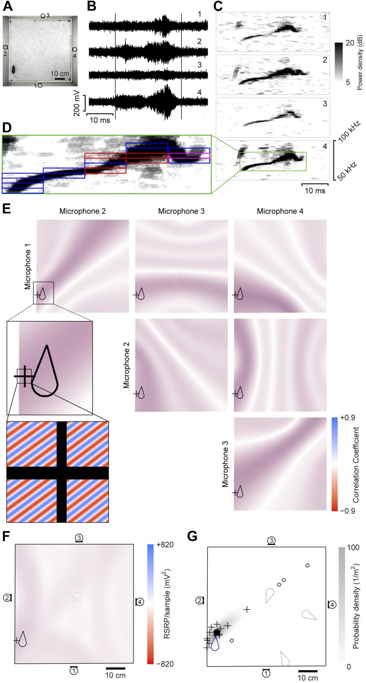
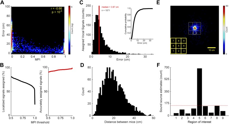
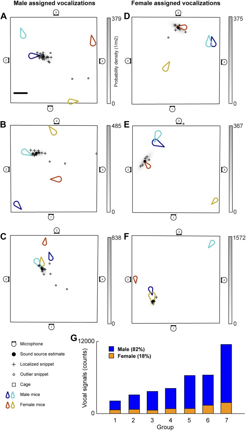
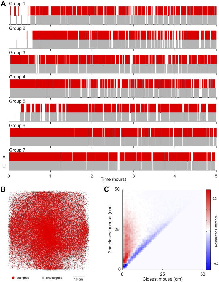
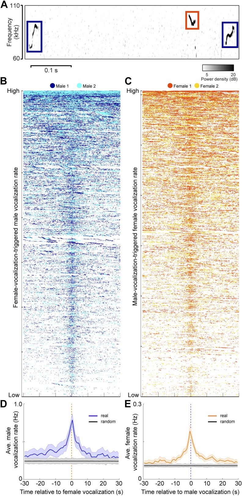
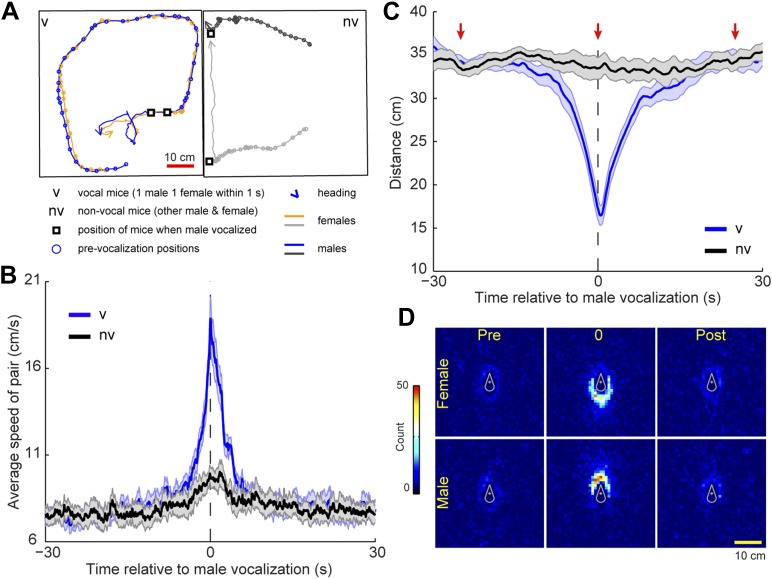
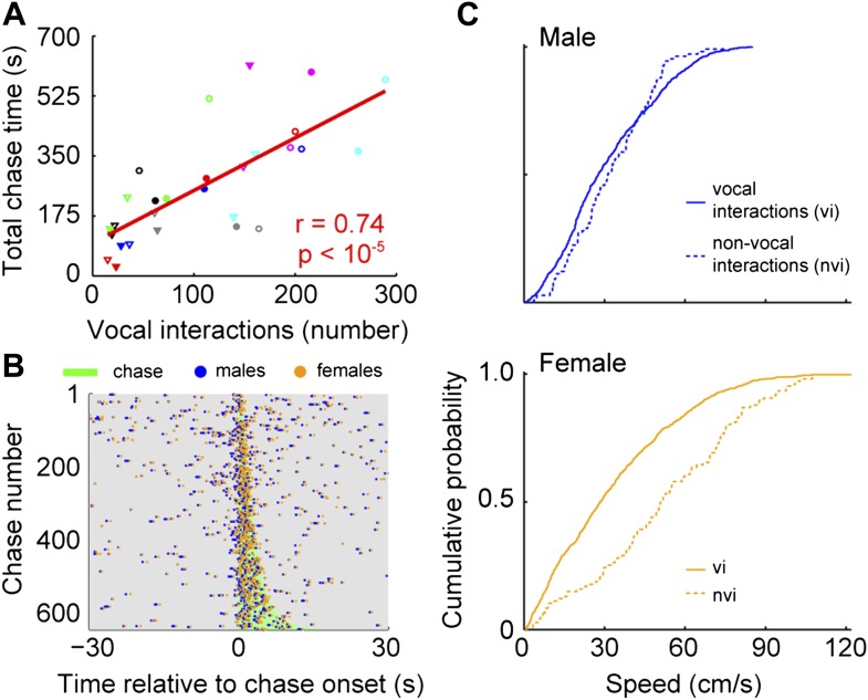
During courtship males attract females with elaborate behaviors. In mice, these displays include ultrasonic vocalizations. Ultrasonic courtship vocalizations were previously attributed to the courting male, despite evidence that both sexes produce virtually indistinguishable vocalizations. Because of this similarity, and the difficulty of assigning vocalizations to individuals, the vocal contribution of each individual during courtship is unknown. To address this question, we developed a microphone array system to localize vocalizations from socially interacting, individual adult mice. With this system, we show that female mice vocally interact with males during courtship. Males and females jointly increased their vocalization rates during chases. Furthermore, a female's participation in these vocal interactions may function as a signal that indicates a state of increased receptivity. Our results reveal a novel form of vocal communication during mouse courtship, and lay the groundwork for a mechanistic dissection of communication during social behavior.
Overview
The claims and statistics of this paper haven’t been checked yet.
Run the check — free, no account needed. It reads the open-access text and checks the sources it cites.
Integrity signals
Registry
Cites
Statistics
Figures
Verification
Claims the paper makes
The claims and statistics of this paper haven’t been checked yet.
Run the check — free, no account needed. It reads the open-access text and checks the sources it cites.
Claims other papers make about this one
Each is checked against this paper’s own text: does it say what the citing paper says it does?
The source backs part of the claim, not all of it — or backs it for a different population, condition or comparison.
In the citing paper
“Similarly, male mice alter behavior in response to female USVs, and these calls contain information about the female’s reproductive receptivity [92,93].”
From The Neurobiology of Love and Pair Bonding from Human and Animal Perspectives (2023) · cites this paper as [92]
Experimental — accuracy not yet measured
Self-check
Percentages, sums and reported differences re-computed from the paper’s own numbers.
The self-check needs the paper’s full text.
Citations
Cites
Principles of animal communication
(2012) · Choice Reviews Online · doi:10.5860/choice.49-5059 · Cited by 2,544
Sexual attractivity, proceptivity, and receptivity in female mammals
Beach, F. A. (1976) · Hormones and Behavior · doi:10.1016/0018-506x(76)90008-8 · Cited by 1,148 · cited 1×
“This is akin to other species; receptive females slow down permitting the courting male to approach and mate (McGill, 1962; Beach, 1976; Hall, 1994; Kowalski et al., 2004; Szykman et al., 2007).”
BackgroundSpectral Analysis for Physical Applications: Multitaper and Conventional Univariate Techniques.
DSS, Percival, D. B., & Walden, A. T. (1997) · Journal of the American Statistical Association · doi:10.2307/2965609 · Cited by 975
The adaptive value of sociality in mammalian groups
Silk, J. B. (2007) · Philosophical Transactions of the Royal Society B Biological Sciences · doi:10.1098/rstb.2006.1994 · Cited by 842 · cited 1×
“DOI: 10.7554/eLife.06203 1 of 24 between males (Silk, 2007).”
InfluentialPrinciples of Animal Communication
Howard, R. W. (1999) · American Entomologist · doi:10.1093/ae/45.2.126 · Cited by 736
Holy, T. E., & Guo, Z. (2005) · PLoS Biology · doi:10.1371/journal.pbio.0030386 · Cited by 673 · cited 2×
“Second, although mice appear to produce characteristic vocal patterns or songs (Holy and Guo, 2005; Sugimoto et al., 2011; Hoffmann et al., 2012), individual ultrasonic vocalizations are similar across animals, both within and between sexes (Hammerschmidt et al., 2012a).”
BackgroundHall, J. C. (1994) · Science · doi:10.1126/science.8209251 · Cited by 668 · cited 1×
“This is akin to other species; receptive females slow down permitting the courting male to approach and mate (McGill, 1962; Beach, 1976; Hall, 1994; Kowalski et al., 2004; Szykman et al., 2007).”
BackgroundBlumstein, D. T., Mennill, D. J., Clemins, P. J., Girod, L., Yao, K., Patricelli, G. L., Deppe, J. L., Krakauer, A. H., Clark, C. W., Cortopassi, K. A., et al. (2011) · Journal of Applied Ecology · doi:10.1111/j.1365-2664.2011.01993.x · Cited by 657 · cited 2×
“Other systems capitalized on the power of an array to determine the number of animals hidden in dense terrain (Celis-Murillo et al., 2009; Blumstein et al., 2011) or map the boundaries of an animal’s territory (Kirschel et al.”
BackgroundJAABA: Interactive machine learning for automatic annotation of animal behavior
Kabra, M., Robie, A. A., Rivera-Alba, M., Branson, S., & Branson, K. (2013) · Nature Methods · doi:10.1038/nmeth.2281 · Cited by 644 · cited 2×
“An automated classifier (Janelia Automatic Animal Behavior Annotator; JAABA; Kabra et al. (2013), http://jaaba.sourceforge.net) was used for identifying events when a female mouse was being followed.”
Method(2007) · PubMed · Cited by 597
Fish can infer social rank by observation alone
Grosenick, L., Clement, T. S., & Fernald, R. D. (2007) · Nature · doi:10.1038/nature05511 · Cited by 556 · cited 2×
“Transfer of social information occurs over a wide range of timescales, from short-term information about an individual’s current motivational state (Moles and D’Amato F, 2000) to longer-term information about dominance status (Ficken et al., 1987; Grosenick et al., 2007) or fertility (Leong et al.”
BackgroundUltrasonic Communication by Animals
Sales, G., & Pye, D. (1974) · Springer eBooks · doi:10.1007/978-94-011-6901-1 · Cited by 539 · cited 1×
“Mice produce ultrasonic vocalizations in many social contexts including establishment of territory, resident–intruder interactions, pup care, juvenile play, social reunion, and mating (Sales and Pye, 1974).”
BackgroundA functional circuit underlying male sexual behaviour in the female mouse brain
Kimchi, T., Xu, J., & Dulac, C. (2007) · Nature · doi:10.1038/nature06089 · Cited by 445 · cited 1×
“Moreover, it is known that female mice possess the neural circuitry necessary to emit USVs during interactions with males because surgical or genetic lesions to the vomeronasal organ unmask this behavior (Kimchi et al., 2007).”
BackgroundA review of hypotheses for the functions of avian duetting
Hall, M. L. (2004) · Behavioral Ecology and Sociobiology · doi:10.1007/s00265-003-0741-x · Cited by 391 · cited 1×
“Most studies have found that vocal behavior is either important for joint territorial defense or maintaining affiliation, particularly between mated pairs (Hall, 2004).”
BackgroundAbolition of male sexual behaviors in mice lacking estrogen receptors α and β (αβERKO)
Ogawa, S., Chester, A. E., Hewitt, S. C., Walker, V. R., Gustafsson, J.-Α., Smithies, O., Korach, K. S., & Pfaff, D. W. (2000) · Proceedings of the National Academy of Sciences · doi:10.1073/pnas.250473597 · Cited by 293
Spectral Analysis for Physical Applications: Multitaper and Conventional Univariate Techniques
Cox, D. D., Percival, D. B., & Walden, A. T. (1996) · Technometrics · doi:10.2307/1270624 · Cited by 292
Conceptual Challenges and Directions for Social Neuroscience
Adolphs, R. (2010) · Neuron · doi:10.1016/j.neuron.2010.03.006 · Cited by 287 · cited 1×
“These interactions are supported by information exchange through a variety of sensory modalities (Adolphs, 2010).”
BackgroundMultivariate Outlier Detection and Robust Covariance Matrix Estimation
Peña, D., & Prieto, F. J. (2001) · Technometrics · doi:10.1198/004017001316975899 · Cited by 279
Ultrasound and mating behaviour in rodents with some observations on other behavioural situations
Sales, G. (1972) · Journal of Zoology · doi:10.1111/j.1469-7998.1972.tb01345.x · Cited by 268 · cited 4×
“Furthermore, a female’s participation in these vocal interactions may function as a signal that indicates a state of increased receptivity.”
BackgroundInfluentialVariable female preferences drive complex male displays
Coleman, S. W., Patricelli, G. L., & Borgia, G. (2004) · Nature · doi:10.1038/nature02419 · Cited by 246 · cited 1×
“Female responsiveness modulates male mating behavior throughout the animal kingdom (Coleman et al., 2004; Higham et al., 2009; Akre and Ryan, 2011).”
BackgroundNonverbal courtship patterns in women
Moore, M. M. (1985) · Ethology and Sociobiology · doi:10.1016/0162-3095(85)90016-0 · Cited by 245 · cited 1×
“A similar interdependence of behavior between partners occurs in the early stages of human courtship, where a female’s non-verbal displays modulate a male’s approach behavior (Moore, 1985).”
BackgroundThe Adaptive Significance of a Complex Vocal Repertoire in a Neotropical Frog
Rand, A. S., & Ryan, M. J. (1981) · Zeitschrift für Tierpsychologie · doi:10.1111/j.1439-0310.1981.tb01923.x · Cited by 235
Weissbrod, A., Shapiro, A., Vasserman, G., Edry, L., Dayan, M., Yitzhaky, A., Hertzberg, L., Feinerman, O., & Kimchi, T. (2013) · Nature Communications · doi:10.1038/ncomms3018 · Cited by 235 · cited 3×
“Moreover, mice living in large populations for extended periods exhibit social interactions that are affected by the dynamics of multiple group members (Shemesh et al., 2013) and complex dominance hierarchies (Weissbrod et al., 2013).”
BackgroundFemale Choice and Mating System of the Brown Capuchin Monkey Cebus apella (Primates: Cebidae)
Janson, C. H. (1984) · Zeitschrift für Tierpsychologie · doi:10.1111/j.1439-0310.1984.tb00098.x · Cited by 227 · cited 2×
“Interactions between males and females during courtship also occur in the vocal domain (Janson, 1984; Tobias et al., 1998; Garamszegi et al., 2007).”
BackgroundFemale mice respond to male ultrasonic ‘songs’ with approach behaviour
Hammerschmidt, K., Radyushkin, K., Ehrenreich, H., & Fischer, J. (2009) · Biology Letters · doi:10.1098/rsbl.2009.0317 · Cited by 226 · cited 2×
“, 2010) or whistle-like control sounds (Hammerschmidt et al., 2009).”
BackgroundSexual Behavior in Three Inbred Strains of Mice
McGill, T. E. (1962) · Behaviour · doi:10.1163/156853962x00087 · Cited by 220 · cited 1×
“This is akin to other species; receptive females slow down permitting the courting male to approach and mate (McGill, 1962; Beach, 1976; Hall, 1994; Kowalski et al., 2004; Szykman et al., 2007).”
BackgroundHigh-order social interactions in groups of mice
Shemesh, Y., Sztainberg, Y., Forkosh, O., Shlapobersky, T., Chen, A., & Schneidman, E. (2013) · eLife · doi:10.7554/elife.00759 · Cited by 213 · cited 3×
“Moreover, mice living in large populations for extended periods exhibit social interactions that are affected by the dynamics of multiple group members (Shemesh et al., 2013) and complex dominance hierarchies (Weissbrod et al., 2013).”
BackgroundLife History AND BIOECONOMY OF THE House Mouse
Berry, R. J., & Bronson, F. H. (1992) · Biological reviews/Biological reviews of the Cambridge Philosophical Society · doi:10.1111/j.1469-185x.1992.tb01192.x · Cited by 202 · cited 1×
“DOI: 10.7554/eLife.06203.001”
InfluentialVan Oortmerssen, G. A. (1971) · Behaviour · doi:10.1163/156853971x00014 · Cited by 201 · cited 1×
“This behavior strongly resembles a chase, a fundamental component of mouse courtship (Van Oortmerssen, 1971).”
BackgroundFemale behavior is affected by male ultrasonic vocalizations in house mice
Pomerantz, S. M., Núñez, A. A., & Bean, N. J. (1983) · Physiology & Behavior · doi:10.1016/0031-9384(83)90101-4 · Cited by 198 · cited 2×
“, 2010), female mice spend more time near vocalizing males than mute males (Pomerantz et al., 1983), and female mice preferentially approach a speaker playing male vocalizations rather than a speaker playing background noise (Musolf et al.”
BackgroundChabout, J., Serreau, P., Ey, E., Bellier, L., Aubin, T., Bourgeron, T., & Granon, S. (2012) · PLoS ONE · doi:10.1371/journal.pone.0029401 · Cited by 197 · cited 3×
“First, there is no obvious visual sign that a mouse is producing a USV (Chabout et al., 2012).”
BackgroundZhang, C., Florencio, D. A. F., Ba, D. E., & Zhang, Z. (2008) · IEEE Transactions on Multimedia · doi:10.1109/tmm.2008.917406 · Cited by 192 · cited 2×
“Mouse sound source estimation was performed using a procedure similar to that of Zhang et al. (2008).”
MethodUltrasonic emissions: Do they facilitate courtship of mice?
Whitney, G., Coble, J. R., Stockton, M. D., & Tilson, E. F. (1973) · Journal of Comparative and Physiological Psychology · doi:10.1037/h0034899 · Cited by 186 · cited 15×
“Moreover, it is known that female mice possess the neural circuitry necessary to emit USVs during interactions with males because surgical or genetic lesions to the vomeronasal organ unmask this behavior (Kimchi et al., 2007).”
BackgroundResultInfluentialUsing soundscape recordings to estimate bird species abundance, richness, and composition
Celis‐Murillo, A., Deppe, J. L., & Allen, M. F. (2009) · Journal of Field Ornithology · doi:10.1111/j.1557-9263.2009.00206.x · Cited by 186 · cited 1×
“courting male, despite evidence that both sexes produce virtually indistinguishable vocalizations.”
BackgroundRapping, a female receptive call, initiates male–female duets in the South African clawed frog
Tobias, M. L., Viswanathan, S. S., & Kelley, D. B. (1998) · Proceedings of the National Academy of Sciences · doi:10.1073/pnas.95.4.1870 · Cited by 173 · cited 1×
“Interactions between males and females during courtship also occur in the vocal domain (Janson, 1984; Tobias et al., 1998; Garamszegi et al., 2007).”
BackgroundBat serenades—complex courtship songs of the sac-winged bat (Saccopteryx bilineata)
Behr, O., & von Helversen, O. (2004) · Behavioral Ecology and Sociobiology · doi:10.1007/s00265-004-0768-7 · Cited by 171 · cited 1×
“To address this question, we developed a microphone array system to localize vocalizations from socially interacting, individual adult mice.”
BackgroundThe role of ultrasonic vocalizations in mouse communication
Portfors, C. V., & Perkel, D. J. (2014) · Current Opinion in Neurobiology · doi:10.1016/j.conb.2014.07.002 · Cited by 170
Female Presence and Estrous State Influence Mouse Ultrasonic Courtship Vocalizations
Hanson, J. L., & Hurley, L. M. (2012) · PLoS ONE · doi:10.1371/journal.pone.0040782 · Cited by 169 · cited 1×
“Furthermore, a female’s participation in these vocal interactions may function as a signal that indicates a state of increased receptivity.”
BackgroundMoles, A., Costantini, F., Garbugino, L., Zanettini, C., & D’Amato, F. R. (2007) · Behavioural Brain Research · doi:10.1016/j.bbr.2007.01.020 · Cited by 167 · cited 1×
“However, females have been reported to vocalize at high rates during same sex interactions (Maggio and Whitney, 1985; Moles et al., 2007).”
BackgroundDynamic sensory cues shape song structure in Drosophila
Coen, P., Clemens, J., Weinstein, A. J., Pacheco, D. A., Deng, Y., & Murthy, M. (2014) · Nature · doi:10.1038/nature13131 · Cited by 166 · cited 1×
“For example, inDrosophila melanogaster, males modulate their song patterning in response to variation in sensory cues about the female’s position and motion (Coen et al., 2014).”
BackgroundAutomated multi-day tracking of marked mice for the analysis of social behaviour
Ohayon, S., Avni, O., Taylor, A. L., Perona, P., & Egnor, S. E. R. (2013) · Journal of Neuroscience Methods · doi:10.1016/j.jneumeth.2013.05.013 · Cited by 154 · cited 3×
“At least one week prior to the start of the recordings, mice were marked with distinctive patterns for identification by applying harmless hair bleach to the fur (Ohayon et al., 2013).”
BackgroundMethodInfluentialUltrasonic vocalizing by adult female mice (Mus musculus).
Maggio, J. C., & Whitney, G. (1985) · Journal of comparative psychology · doi:10.1037/0735-7036.99.4.420 · Cited by 154
Sugimoto, H., Okabe, S., Kato, M., Koshida, N., Shiroishi, T., Mogi, K., Kikusui, T., & Koide, T. (2011) · PLoS ONE · doi:10.1371/journal.pone.0022093 · Cited by 152 · cited 2×
“Second, although mice appear to produce characteristic vocal patterns or songs (Holy and Guo, 2005; Sugimoto et al., 2011; Hoffmann et al., 2012), individual ultrasonic vocalizations are similar across animals, both within and between sexes (Hammerschmidt et al., 2012a).”
Background40- and 70-kHz Vocalizations of Mice (Mus musculus) during Copulation
White, N. R., Prasad, M., Barfield, R. J., & Nyby, J. (1998) · Physiology & Behavior · doi:10.1016/s0031-9384(97)00484-8 · Cited by 151 · cited 2×
“…use pairs of mice (Bean et al., 1981; Choi et al., 2011; D’Amato and Moles, 2001; Hammerschmidt et al., 2012b; Nunez et al., 1978; Nyby et al., 1976; Ogawa et al., 2000; Pomerantz and Clemens, 1981; Rotschafer et al., 2012; Scattoni et al., 2008; Warburton et al., 1989; White et al., 1998).”
BackgroundMethodUltrasonic courtship vocalizations in wild house mice, Mus musculus musculus
Musolf, K., Hoffmann, F., & Penn, D. J. (2010) · Animal Behaviour · doi:10.1016/j.anbehav.2009.12.034 · Cited by 148 · cited 4×
“…during mating (Sewell, 1972; Hanson and Hurley, 2012), urine from females but not males stimulates vocal production in males (Nyby et al., 1979; Musolf et al., 2010), female mice spend more time near vocalizing males than mute males (Pomerantz et al., 1983), and female mice preferentially…”
BackgroundInfluentialUltrasonic vocalizations during sex behavior of male house mice (Mus musculus): A description
Nyby, J. (1983) · Behavioral and Neural Biology · doi:10.1016/s0163-1047(83)90722-7 · Cited by 142 · cited 1×
“Supporting previous work (Sewell, 1972; Nyby, 1983; Chabout et al., 2012), we directly showed that male mice vocalize in the presence of freely moving female mice.”
Reduced ultrasonic vocalizations in vasopressin 1b knockout mice
Scattoni, M. L., McFarlane, H. G., Zhodzishsky, V., Caldwell, H. K., YOUNG, W., Ricceri, L., & Crawley, J. N. (2007) · Behavioural Brain Research · doi:10.1016/j.bbr.2007.09.034 · Cited by 134 · cited 2×
“…use pairs of mice (Bean et al., 1981; Choi et al., 2011; D’Amato and Moles, 2001; Hammerschmidt et al., 2012b; Nunez et al., 1978; Nyby et al., 1976; Ogawa et al., 2000; Pomerantz and Clemens, 1981; Rotschafer et al., 2012; Scattoni et al., 2008; Warburton et al., 1989; White et al., 1998).”
BackgroundMethodRotschafer, S. E., Trujillo, M. S., Dansie, L. E., Ethell, I. M., & Razak, K. A. (2012) · Brain Research · doi:10.1016/j.brainres.2011.12.041 · Cited by 130 · cited 2×
“…use pairs of mice (Bean et al., 1981; Choi et al., 2011; D’Amato and Moles, 2001; Hammerschmidt et al., 2012b; Nunez et al., 1978; Nyby et al., 1976; Ogawa et al., 2000; Pomerantz and Clemens, 1981; Rotschafer et al., 2012; Scattoni et al., 2008; Warburton et al., 1989; White et al., 1998).”
BackgroundMethodHammerschmidt, K., Radyushkin, K., Ehrenreich, H., & Fischer, J. (2012) · PLoS ONE · doi:10.1371/journal.pone.0041133 · Cited by 127 · cited 1×
“DOI: 10.7554/eLife.06203.001”
InfluentialMice do not require auditory input for the normal development of their ultrasonic vocalizations
Hammerschmidt, K., Reisinger, E., Westekemper, K., Ehrenreich, L., Strenzke, N., & Fischer, J. (2012) · BMC Neuroscience · doi:10.1186/1471-2202-13-40 · Cited by 123 · cited 5×
“…vocal behavior of adult mice, most experimental paradigms use pairs of mice (Bean et al., 1981; Choi et al., 2011; D’Amato and Moles, 2001; Hammerschmidt et al., 2012b; Nunez et al., 1978; Nyby et al., 1976; Ogawa et al., 2000; Pomerantz and Clemens, 1981; Rotschafer et al., 2012;…”
BackgroundMethodInfluentialFertility Advertisement in Birds: a Means of Inciting Male‐male Competition?
Montgomerie, R., & Thornhill, R. (1989) · Ethology · doi:10.1111/j.1439-0310.1989.tb00767.x · Cited by 123 · cited 1×
“As for the role of female vocalizations in courtship, many believe a female’s participation may serve as an indication of her receptivity (Janson, 1984) or may encourage competition between males (Montgomerie and Thornhill, 1989).”
BackgroundUltrasonic frogs show hyperacute phonotaxis to female courtship calls
Shen, J., Feng, A. S., Xu, Z.-M., Yu, Z., Arch, V. S., Yu, X.-J., & Narins, P. M. (2008) · Nature · doi:10.1038/nature06719 · Cited by 122 · cited 2×
“…(Blank et al., 2014), songbirds stimulate reproductive activity in females by singing (Bentley et al., 2000), sac-winged bats produce complex serenades during sexual displays (Behr and von Helversen, 2004), and anurans phonotaxis towards ultrasonic courtship vocalizations (Shen et al., 2008).”
BackgroundMennill, D. J., Burt, J. M., Fristrup, K. M., & Vehrencamp, S. L. (2006) · The Journal of the Acoustical Society of America · doi:10.1121/1.2184988 · Cited by 122 · cited 1×
“In the past, microphone arrays have been used to study the acoustic features of many species (Payne et al., 2003;Mennill et al., 2006; Chiu et al., 2010; Collier et al., 2010; Kalcounis-Rueppell et al., 2010).”
MethodFitness effects of communal rearing in house mice: the role of relatedness versus familiarity
König, B. (1994) · Animal Behaviour · doi:10.1006/anbe.1994.1381 · Cited by 121
Ultrasonic vocalisations facilitate sexual behaviour of female rats
McIntosh, T. K., Barfield, R. J., & Geyer, L. A. (1978) · Nature · doi:10.1038/272163a0 · Cited by 117 · cited 1×
“In rodents, reports indicate that USVs are important for female receptivity during estrus (Floody et al., 1977; McIntosh et al., 1978) and, therefore two hours prior to the anticipated start of the experiment, non-invasive lavage and cytological assessment of vaginal cells were performed.”
MethodFloody, O. R., Pfaff, D. W., & Lewis, C. D. (1977) · Journal of Comparative and Physiological Psychology · doi:10.1037/h0077361 · Cited by 116 · cited 2×
“In rodents, reports indicate that USVs are important for female receptivity during estrus (Floody et al., 1977; McIntosh et al., 1978) and, therefore two hours prior to the anticipated start of the experiment, non-invasive lavage and cytological assessment of vaginal cells were performed.”
BackgroundMethodThe evolution of song in female birds in Europe
Garamszegi, L. Z., Pavlova, D. Z., Eens, M., & Møller, A. P. (2006) · Behavioral Ecology · doi:10.1093/beheco/arl047 · Cited by 116 · cited 1×
“Interactions between males and females during courtship also occur in the vocal domain (Janson, 1984; Tobias et al., 1998; Garamszegi et al., 2007).”
BackgroundBentley, G. E., Wingfield, J. C., Morton, M. L., & Ball, G. F. (2000) · Hormones and Behavior · doi:10.1006/hbeh.2000.1573 · Cited by 113 · cited 2×
“, 2014), songbirds stimulate reproductive activity in females by singing (Bentley et al., 2000), sac-winged bats produce complex serenades during sexual displays (Behr and von Helversen, 2004), and anurans phonotaxis towards ultrasonic courtship vocalizations (Shen et al.”
BackgroundElicitation of male mouse (Mus musculus) ultrasonic vocalizations: I. Urinary cues.
Nyby, J., Wysocki, C. J., Whitney, G., Dizinno, G. A., & Schneider, J. E. (1979) · Journal of Comparative and Physiological Psychology · doi:10.1037/h0077623 · Cited by 110 · cited 2×
“For example, USVs occur during mating (Sewell, 1972; Hanson and Hurley, 2012), urine from females but not males stimulates vocal production in males (Nyby et al., 1979; Musolf et al., 2010), female mice spend more time near vocalizing males than mute males (Pomerantz et al.”
BackgroundUltrasonic vocalization of the female rat (Rattus norvegicus) during mating
Thomas, D. A., & Barfield, R. J. (1985) · Animal Behaviour · doi:10.1016/s0003-3472(85)80002-6 · Cited by 103
Social status and ultrasonic vocalizations of male mice
Nyby, J., Dizinno, G. A., & Whitney, G. (1976) · Behavioral Biology · doi:10.1016/s0091-6773(76)92198-2 · Cited by 102 · cited 2×
“When examining the ultrasonic vocal behavior of adult mice, most experimental paradigms use pairs of mice (Bean et al., 1981; Choi et al., 2011; D’Amato and Moles, 2001; Hammerschmidt et al., 2012b; Nunez et al., 1978; Nyby et al., 1976; Ogawa et al., 2000; Pomerantz and Clemens, 1981; Rotschafer et al., 2012; Scatton…”
MethodFemale reproductive signaling, and male mating behavior, in the olive baboon
Higham, J. P., Semple, S., MacLarnon, A. M., Heistermann, M., & Ross, C. (2008) · Hormones and Behavior · doi:10.1016/j.yhbeh.2008.08.007 · Cited by 99 · cited 1×
“Female responsiveness modulates male mating behavior throughout the animal kingdom (Coleman et al., 2004; Higham et al., 2009; Akre and Ryan, 2011).”
BackgroundHoffmann, F., Musolf, K., & Penn, D. J. (2011) · Physiology & Behavior · doi:10.1016/j.physbeh.2011.10.011 · Cited by 97 · cited 2×
“Second, although mice appear to produce characteristic vocal patterns or songs (Holy and Guo, 2005; Sugimoto et al., 2011; Hoffmann et al., 2012), individual ultrasonic vocalizations are similar across animals, both within and between sexes (Hammerschmidt et al., 2012a).”
BackgroundPayne, K. B., Thompson, M. E., & Kramer, L. (2003) · African Journal of Ecology · doi:10.1046/j.1365-2028.2003.00421.x · Cited by 95 · cited 1×
“In the past, microphone arrays have been used to study the acoustic features of many species (Payne et al., 2003;Mennill et al., 2006; Chiu et al., 2010; Collier et al., 2010; Kalcounis-Rueppell et al., 2010).”
MethodAnderson, P. K. (1961) · Transactions of the New York Academy of Sciences · doi:10.1111/j.2164-0947.1961.tb01373.x · Cited by 93 · cited 2×
“DOI: 10.7554/eLife.06203.001”
BackgroundInfluentialUltrasonic vocalization by female mice in the presence of a conspecific carrying food cues
Moles, A., & D'Amato, F. R. (2000) · Animal Behaviour · doi:10.1006/anbe.2000.1504 · Cited by 91
Ultrasonic vocalizations as an index of social memory in female mice.
D'Amato, F. R., & Moles, A. (2001) · Behavioral Neuroscience · doi:10.1037//0735-7044.115.4.834 · Cited by 91 · cited 1×
“DOI: 10.7554/eLife.06203.001”
InfluentialUltrasonic vocalizations as an index of social memory in female mice.
D'Amato, F. R., & Moles, A. (2001) · Behavioral Neuroscience · doi:10.1037/0735-7044.115.4.834 · Cited by 79
Kalcounis‐Rueppell, M. C., Petric, R., Briggs, J. R., Carney, C., Marshall, M. M., Willse, J. T., Rueppell, O., Ribble, D. O., & Crossland, J. P. (2010) · PLoS ONE · doi:10.1371/journal.pone.0009705 · Cited by 77
Warburton, V. L., Sales, G., & Milligan, S. R. (1989) · Physiology & Behavior · doi:10.1016/0031-9384(89)90164-9 · Cited by 74 · cited 16×
“Moreover, it is known that female mice possess the neural circuitry necessary to emit USVs during interactions with males because surgical or genetic lesions to the vomeronasal organ unmask this behavior (Kimchi et al., 2007).”
BackgroundMethodResultInfluentialKirschel, A. N. G., Cody, M. L., Harlow, Z. T., Promponas, V. J., Vallejo, E. E., & TAYLOR, C. E. (2011) · Ibis · doi:10.1111/j.1474-919x.2011.01102.x · Cited by 70 · cited 2×
“…the number of animals hidden in dense terrain (Celis-Murillo et al., 2009; Blumstein et al., 2011) or map the boundaries of an animal’s territory (Kirschel et al., 2011), whereas our system was specifically designed to link, with high resolution and accuracy, the vocal and social behaviors of…”
BackgroundNúñez, A. A., Nyby, J., & Whitney, G. (1978) · Hormones and Behavior · doi:10.1016/0018-506x(78)90030-2 · Cited by 69 · cited 2×
“…mice, most experimental paradigms use pairs of mice (Bean et al., 1981; Choi et al., 2011; D’Amato and Moles, 2001; Hammerschmidt et al., 2012b; Nunez et al., 1978; Nyby et al., 1976; Ogawa et al., 2000; Pomerantz and Clemens, 1981; Rotschafer et al., 2012; Scattoni et al., 2008; Warburton et…”
MethodChiu, C., Reddy, P. V., Xian, W., Krishnaprasad, P. S., & Moss, C. F. (2010) · Journal of Experimental Biology · doi:10.1242/jeb.044818 · Cited by 66 · cited 1×
“In the past, microphone arrays have been used to study the acoustic features of many species (Payne et al., 2003;Mennill et al., 2006; Chiu et al., 2010; Collier et al., 2010; Kalcounis-Rueppell et al., 2010).”
MethodJones, R. B., & Nowell, N. W. (1989) · Aggressive Behavior · doi:10.1002/ab.2480150404 · Cited by 62
Leong, K. M., Ortolani, A., Graham, L. H., & Savage, A. (2003) · Hormones and Behavior · doi:10.1016/s0018-506x(03)00025-4 · Cited by 61 · cited 1×
“…of social information occurs over a wide range of timescales, from short-term information about an individual’s current motivational state (Moles and D’Amato F, 2000) to longer-term information about dominance status (Ficken et al., 1987; Grosenick et al., 2007) or fertility (Leong et al., 2003).”
BackgroundEffects of medial preoptic lesions on male mouse ultrasonic vocalizations and copulatory behavior
Bean, N. J., Núñez, A. A., & Conner, R. L. (1981) · Brain Research Bulletin · doi:10.1016/s0361-9230(81)80033-0 · Cited by 60
Female túngara frogs elicit more complex mating signals from males
Akre, K. L., & Ryan, M. J. (2011) · Behavioral Ecology · doi:10.1093/beheco/arr065 · Cited by 43 · cited 1×
“Female responsiveness modulates male mating behavior throughout the animal kingdom (Coleman et al., 2004; Higham et al., 2009; Akre and Ryan, 2011).”
BackgroundMartínez-Rivera, C. C., & Gerhardt, H. C. (2008) · Behavioral Ecology and Sociobiology · doi:10.1007/s00265-008-0650-0 · Cited by 42 · cited 2×
“However, females have been reported to vocalize at high rates during same sex interactions (Maggio and Whitney, 1985; Moles et al., 2007).”
BackgroundPlaying to an audience: the social environment influences aggression and victory displays
Fitzsimmons, L. P., & Bertram, S. M. (2013) · Biology Letters · doi:10.1098/rsbl.2013.0449 · Cited by 41 · cited 1×
“Group size influences the behavior of individual animals (Fitzsimmons and Bertram, 2013; Shen et al., 2014).”
BackgroundInfluence of the female sexual cycle on BALB/c mouse calling behaviour during mating
Barthélemy, M., Gourbal, B., Gabrion, C., & Petit, G. (2004) · Die Naturwissenschaften · doi:10.1007/s00114-004-0501-4 · Cited by 39 · cited 2×
“…studies have addressed the difficulty in determining the source by assuming a single mouse produced the majority of the observed vocalizations (Barthelemy et al., 2004; Choi et al., 2011; Hanson and Hurley, 2012), or by experimentally preventing one mouse from vocalizing (Whitney et al.,…”
BackgroundResultKarim, B. O., Landolfi, J. A., Christian, A., Arbona, R. J. R., Qiu, W., McAlonis‐Downes, M., Eyabi, P. O., Khan, K. A., Dicello, J. F., Mann, J. F., et al. (2003) · PubMed · Cited by 39
Context-Related Acoustic Variation in Male Fallow Deer (Dama dama) Groans
Charlton, B. D., & Reby, D. (2011) · PLoS ONE · doi:10.1371/journal.pone.0021066 · Cited by 37 · cited 1×
“For example, in a variety of species, the full range of a male’s vocal repertoire only occurs when multiple males are present (Rand and Ryan, 1981; Martinez-Rivera and Gerhardt, 2008; Charlton and Reby, 2011).”
BackgroundGroup Size and Social Conflict in Complex Societies
Shen, S., Akçay, E., & Rubenstein, D. R. (2013) · The American Naturalist · doi:10.1086/674378 · Cited by 35 · cited 1×
“Group size influences the behavior of individual animals (Fitzsimmons and Bertram, 2013; Shen et al., 2014).”
BackgroundA Complex Vocalization of the Black-Capped Chickadee. II. Repertoires, Dominance and Dialects
Ficken, M. S., Weise, C. M., & Reinartz, J. A. (1987) · Ornithological Applications · doi:10.2307/1368640 · Cited by 34 · cited 2×
“Transfer of social information occurs over a wide range of timescales, from short-term information about an individual’s current motivational state (Moles and D’Amato F, 2000) to longer-term information about dominance status (Ficken et al., 1987; Grosenick et al., 2007) or fertility (Leong et al.”
BackgroundCourtship and mating in free-living spotted hyenas
Gunther, M. S., HORN, R. C. V., Engh, A. L., Boydston, E. E., & Holekamp, K. E. (2007) · Behaviour · doi:10.1163/156853907781476418 · Cited by 32 · cited 1×
“This is akin to other species; receptive females slow down permitting the courting male to approach and mate (McGill, 1962; Beach, 1976; Hall, 1994; Kowalski et al., 2004; Szykman et al., 2007).”
BackgroundPomerantz, S. M., & Clemens, L. G. (1981) · Physiology & Behavior · doi:10.1016/0031-9384(81)90055-x · Cited by 31 · cited 1×
“DOI: 10.7554/eLife.06203.001”
InfluentialCourtship song in Drosophila melanogaster: a differential effect on male–female locomotor activity
Kowalski, S., Aubin, T., & Martin, J. (2004) · Canadian Journal of Zoology · doi:10.1139/z04-102 · Cited by 29 · cited 2×
“We used speed at the time of the male vocalization as a proxy for female receptivity (Kowalski et al., 2004).”
BackgroundMethodNyby, J., Wysocki, C. J., Whitney, G., Dizinno, G. A., Schneider, J. E., & Núñez, A. A. (1981) · Journal of Comparative and Physiological Psychology · doi:10.1037/h0077794 · Cited by 28
Is Alarm Calling Risky? Marmots Avoid Calling from Risky Places
Collier, T. C., Blumstein, D. T., Girod, L., & TAYLOR, C. E. (2010) · Ethology · doi:10.1111/j.1439-0310.2010.01830.x · Cited by 27 · cited 1×
“In the past, microphone arrays have been used to study the acoustic features of many species (Payne et al., 2003;Mennill et al., 2006; Chiu et al., 2010; Collier et al., 2010; Kalcounis-Rueppell et al., 2010).”
MethodTwo genetic loci control syllable sequences of ultrasonic courtship vocalizations in inbred mice
Choi, H., Park, S., & Kim, D. (2011) · BMC Neuroscience · doi:10.1186/1471-2202-12-104 · Cited by 14 · cited 4×
“Previous studies have addressed the difficulty in determining the source by assuming a single mouse produced the majority of the observed vocalizations (Barthelemy et al., 2004; Choi et al., 2011; Hanson and Hurley, 2012), or by experimentally preventing one mouse from vocalizing (Whitney et al.”
BackgroundMethodInfluentialRoaring function in male goitered gazelles
Blank, D. A., Ruckstuhl, K. E., & Yang, W. (2014) · Behavioural Processes · doi:10.1016/j.beproc.2014.05.009 · Cited by 11 · cited 2×
“Gazelles roar during mating displays (Blank et al., 2014), songbirds stimulate reproductive activity in females by singing (Bentley et al., 2000), sac-winged bats produce complex serenades during sexual displays (Behr and von Helversen, 2004), and anurans phonotaxis towards ultrasonic courtship…”
Background
Cited by
Sorted by citations
Neural circuit mechanisms of social behavior
Chen, P., & Hong, W. (2018) · Neuron · doi:10.1016/j.neuron.2018.02.026 · Cited by 527
“…of male courtship songs in mice are correlated with mate choice (Asaba et al., 2014); adult females are known to vocalize in the presence of novel conspecifics and vocally interact with males during courtship and parenting (Hammerschmidt et al., 2012; Liu et al., 2013; Neunuebel et al., 2015).”
Computational Analysis of Behavior
Egnor, S. E. R., & Branson, K. M. (2016) · Annual Review of Neuroscience · doi:10.1146/annurev-neuro-070815-013845 · Cited by 200
“Biologists have deployed a wide array of sensors to capture animal behavior, including infrared sensors (Friedman et al. 1997), microphone arrays (Neunuebel et al. 2015), laser Doppler vibrometry (Elias et al. 2003),…”
BackgroundA Specialized Neural Circuit Gates Social Vocalizations in the Mouse
Tschida, K., Michael, V., Takatoh, J., Han, B.-X., Zhao, S., Sakurai, K., MOONEY, R. D., & Wang, F. (2019) · Neuron · doi:10.1016/j.neuron.2019.05.025 · Cited by 188
Measuring behavior across scales
Berman, G. J. (2018) · BMC Biology · doi:10.1186/s12915-018-0494-7 · Cited by 194
“…dynamics to, for example, audio dynamics through asking what behavioral features predict the performance of a particular song or song type using methods such as general linear models (GLMs) [88–90], and improvements in automated methods have increased the throughput of audio data analysis [91–94].”
MethodAn insular view of the social decision-making network
Rogers-Carter, M. M., & Christianson, J. P. (2019) · Neuroscience & Biobehavioral Reviews · doi:10.1016/j.neubiorev.2019.06.005 · Cited by 121
Metadata
- Authors
- Neunuebel, J. P., Taylor, A. L., Arthur, B. J., & Egnor, S. R.
- Affiliations
- Howard Hughes Medical Institute (US)
- Janelia Research Campus, Howard Hughes Medical Institute, Ashburn, United States
- Corresponding author
- Neunuebel, Joshua P
- Venue
- eLife
- Publisher
- eLife Sciences Publications, Ltd
- Published
- 2015-05-28
- Volume
- 4
- ISSN
- 2050-084X (ISSN-L)
- PMC
- PMC4447045
- OpenAlex
- W2161992654
- Cited by
- 224
- References
- 91
- Citations by year
- 2026: 15 · 2025: 20 · 2024: 24 · 2023: 23 · 2022: 22 · 2021: 22 · 2020: 18 · 2019: 13 · 2018: 24 · 2017: 18 · 2016: 22 · 2015: 3
- FWCI
- 19.33
- Type
- journal article
- Language
- en
- Open access
- gold
- doi.org
- Licence
- Locations
- eLife (publishedVersion, cc-by)
- Europe PMC (PubMed Central) (publishedVersion, cc-by)
- PubMed Central (publishedVersion, cc-by)
- PubMed (publishedVersion)
- DOAJ (DOAJ: Directory of Open Access Journals) (submittedVersion, cc-by-sa)
- Funders
- Howard Hughes Medical Institute (HHMI) (Janelia Research Campus)
- Topics
- Life Sciences › Agricultural and Biological Sciences › Ecology, Evolution, Behavior and Systematics › Animal Vocal Communication and Behavior
- Life Sciences › Agricultural and Biological Sciences › Ecology, Evolution, Behavior and Systematics › Animal Behavior and Reproduction
- Life Sciences › Neuroscience › Endocrine and Autonomic Systems › Neuroendocrine regulation and behavior
- Keywords
- courtship vocalizations, ultrasonic vocalizations, microphone array, vocal communication, chase, social behavior
- MeSH terms
- Animals, Courtship, Female, Male, Mice, Inbred C57BL, Sex Factors, Social Behavior, Ultrasonics, Vocalization, Animal, Mice
About these checks
Registry, retraction, Cites and statistics results are computed, not judged, with one exception: a printed reference that no index lists is read once by a model before it counts as a citation error. Claims are extracted by a model and kept only when their quote appears verbatim in the text; each cited source is then checked, with a model’s help, for whether it says what the claim relies on. Those verdicts can be wrong — read the claim’s quote and the cited source before relying on one.
Statistics and arithmetic are recomputed, not judged.
Confidence bands are shown only for fields calibrated on our annotated test set. None is calibrated yet, so no band is shown.
What counts as a claim ›How we measure confidence ›How we check this ›
Are you an author, or do you see a problem with this page? Request a review
