Cited by 33

The DOI matches its Crossref record; 9 of the 9 references it cites were found in a registry or an index.

GluA4 facilitates cerebellar expansion coding and enables associative memory formation

Kita, Katarzyna, Albergaria, Catarina, Machado, Ana S, Carey, Megan R, Müller, Martin, Delvendahl, Igor·2021·eLife

Published version of a preprint

Abstract

AMPA receptors (AMPARs) mediate excitatory neurotransmission in the central nervous system (CNS) and their subunit composition determines synaptic efficacy. Whereas AMPAR subunits GluA1–GluA3 have been linked to particular forms of synaptic plasticity and learning, the functional role of GluA4 remains elusive. Here, we demonstrate a crucial function of GluA4 for synaptic excitation and associative memory formation in the cerebellum. Notably, GluA4-knockout mice had ~80% reduced mossy fiber to granule cell synaptic transmission. The fidelity of granule cell spike output was markedly decreased despite attenuated tonic inhibition and increased NMDA receptor-mediated transmission. Computational network modeling incorporating these changes revealed that deletion of GluA4 impairs granule cell expansion coding, which is important for pattern separation and associative learning. On a behavioral level, while locomotor coordination was generally spared, GluA4-knockout mice failed to form associative memories during delay eyeblink conditioning. These results demonstrate an essential role for GluA4-containing AMPARs in cerebellar information processing and associative learning.

Overview

The claims and statistics of this paper haven’t been checked yet.

Run the check — free, no account needed. It reads the open-access text and checks the sources it cites.

A few free checks a day · papers already verified open instantly · results are public

Integrity signals

Registry

Crossref · 10.7554/elife.65152

Cites

9 of 9 references verified0 citation errors · 0 not checkable

Statistics

Figures
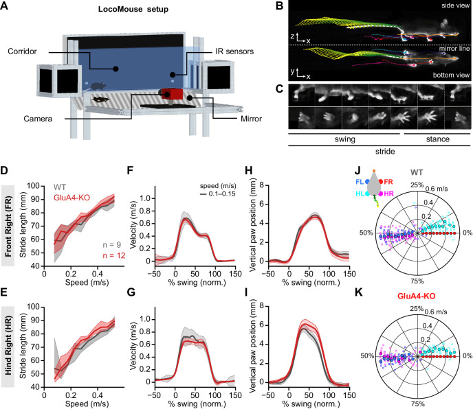
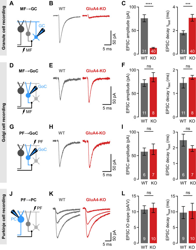
Figure 1. Selective impairment of cerebellar mossy fiber (MF)→granule cell (GC) synapses in GluA4-knockout (GluA4-KO) mice. (A) Schematic of recordings from MF→GC connections. (B) Example excitatory postsynaptic currents (EPSCs) recorded from wild-type (WT) and KO GCs by single MF stimulation. (C) Average EPSC amplitude (left; p < 0.0001; Cohen’s d = −2.23) and average EPSC fast decay time constant (right; p < 0.001; d = 0.84) for WT and KO MF→GC EPSCs. Data are redrawn from Delvendahl et al., 2019. (D) Recordings from MF→Golgi cell (GoC) connections. (E) Example EPSCs upon MF stimulation recorded from GoCs. (F) Average EPSC amplitude (left; p = 0.32; d = 0.49) and fast decay time constant (right; p = 0.33; d = 0.42) for WT and KO MF→GoC EPSCs. (G) Recordings from parallel fiber (PF)→GoC connections. (H) Example EPSCs recorded from GoCs upon PF stimulation. (I) Average EPSC amplitude (left; p = 0.73; d = 0.19) and fast decay time constant (right; p = 0.25; d = −0.73) for WT and KO PF→GoC EPSCs. (J) Recordings from PF→Purkinje cell (PC) connections. (K) Example EPSCs recorded from PCs by stimulating afferent PFs with increasing stimulation strength (displayed stimulation intensities: 7, 12, and 17 V). (L) Average linear slope of the stimulus-response relationship (left; p = 0.79; d = 0.12) and fast decay time constant (right; p = 0.87; d = 0.08) for WT and KO PF→PC EPSCs. Data are means ± SEM.
Figure 1. Selective impairment of cerebellar mossy fiber (MF)→granule cell (GC) synapses in GluA4-knockout (GluA4-KO) mice. (A) Schematic of recordings from MF→GC connections. (B) Example excitatory postsynaptic currents (EPSCs) recorded from wild-type (WT) and KO GCs by single MF stimulation. (C) Average EPSC amplitude (left; p < 0.0001; Cohen’s d = −2.23) and average EPSC fast decay time constant (right; p < 0.001; d = 0.84) for WT and KO MF→GC EPSCs. Data are redrawn from Delvendahl et al., 2019. (D) Recordings from MF→Golgi cell (GoC) connections. (E) Example EPSCs upon MF stimulation recorded from GoCs. (F) Average EPSC amplitude (left; p = 0.32; d = 0.49) and fast decay time constant (right; p = 0.33; d = 0.42) for WT and KO MF→GoC EPSCs. (G) Recordings from parallel fiber (PF)→GoC connections. (H) Example EPSCs recorded from GoCs upon PF stimulation. (I) Average EPSC amplitude (left; p = 0.73; d = 0.19) and fast decay time constant (right; p = 0.25; d = −0.73) for WT and KO PF→GoC EPSCs. (J) Recordings from PF→Purkinje cell (PC) connections. (K) Example EPSCs recorded from PCs by stimulating afferent PFs with increasing stimulation strength (displayed stimulation intensities: 7, 12, and 17 V). (L) Average linear slope of the stimulus-response relationship (left; p = 0.79; d = 0.12) and fast decay time constant (right; p = 0.87; d = 0.08) for WT and KO PF→PC EPSCs. Data are means ± SEM.CC BY · PubMed Central
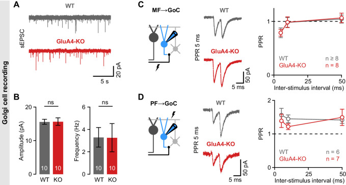
Figure 1—figure supplement 1. Unaltered transmission at excitatory synapses in cerebellar Golgi cells (GoCs). (A) Example spontaneous excitatory postsynaptic current (sEPSC) recordings from wild-type (WT) and GluA4-knockout (GluA4-KO) GoCs. (B) Average sEPSC amplitudes (left; p = 0.96) and frequency (right; p = 0.98) for both genotypes. (C) Left: Schematic of recordings from mossy fiber (MF)→GoC connections. Middle: Example paired-pulses at 5 ms inter-stimulus interval for WT and GluA4-KO. Right: Average paired-pulse ratios (PPR) vs. inter-stimulus interval for both genotypes. (D) Same as (C), but for parallel fiber (PF)→GoC connections. Data are means ± SEM.
Figure 1—figure supplement 1. Unaltered transmission at excitatory synapses in cerebellar Golgi cells (GoCs). (A) Example spontaneous excitatory postsynaptic current (sEPSC) recordings from wild-type (WT) and GluA4-knockout (GluA4-KO) GoCs. (B) Average sEPSC amplitudes (left; p = 0.96) and frequency (right; p = 0.98) for both genotypes. (C) Left: Schematic of recordings from mossy fiber (MF)→GoC connections. Middle: Example paired-pulses at 5 ms inter-stimulus interval for WT and GluA4-KO. Right: Average paired-pulse ratios (PPR) vs. inter-stimulus interval for both genotypes. (D) Same as (C), but for parallel fiber (PF)→GoC connections. Data are means ± SEM.CC BY · PubMed Central
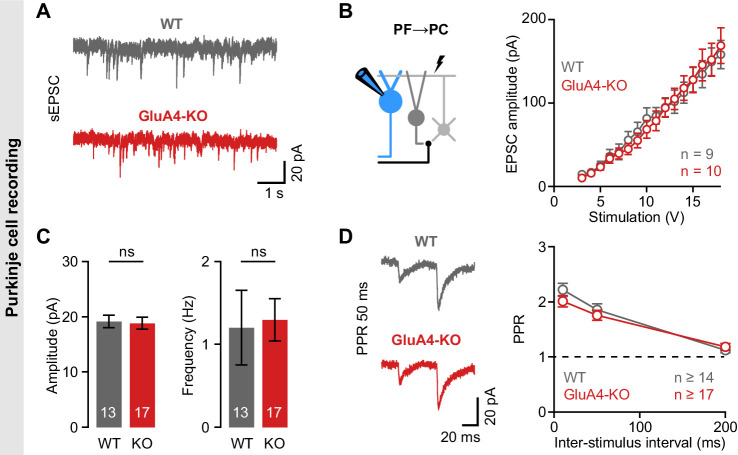
Figure 1—figure supplement 2. Unaltered transmission at excitatory synapses in cerebellar Purkinje cells (PCs). (A) Example spontaneous excitatory postsynaptic current (sEPSC) recordings from wild-type (WT) and GluA4-knockout (GluA4-KO) PCs. (B) Average sEPSC amplitude (left; p = 0.84) and frequency (right; p = 0.0.85) for both genotypes. (C) Left: Schematic of EPSC recordings from parallel fiber (PF)→PC connections. Right: PF→PC EPSC amplitude as a function of stimulation intensity. (D) Left: Example paired-pulses at 50 ms inter-stimulus interval. Right: Average paired-pulse ratio (PPR) vs. inter-stimulus interval for WT and GluA4-KO PCs. Data are means ± SEM.
Figure 1—figure supplement 2. Unaltered transmission at excitatory synapses in cerebellar Purkinje cells (PCs). (A) Example spontaneous excitatory postsynaptic current (sEPSC) recordings from wild-type (WT) and GluA4-knockout (GluA4-KO) PCs. (B) Average sEPSC amplitude (left; p = 0.84) and frequency (right; p = 0.0.85) for both genotypes. (C) Left: Schematic of EPSC recordings from parallel fiber (PF)→PC connections. Right: PF→PC EPSC amplitude as a function of stimulation intensity. (D) Left: Example paired-pulses at 50 ms inter-stimulus interval. Right: Average paired-pulse ratio (PPR) vs. inter-stimulus interval for WT and GluA4-KO PCs. Data are means ± SEM.CC BY · PubMed Central
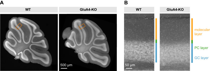
Figure 1—figure supplement 3. Unaltered gross cerebellar organization. (A) DAPI stained sagittal cerebellar sections of wild-type (WT) and GluA4-knockout (GluA4-KO) mice. (B) Higher magnifications of (A) as indicated by orange boxes. Relative thickness of granule cell (GC) layer, Purkinje cell (PC) layer, and molecular layer was not changed in GluA4-KO mice. Similar results were obtained in n = 5 experiments.
Figure 1—figure supplement 3. Unaltered gross cerebellar organization. (A) DAPI stained sagittal cerebellar sections of wild-type (WT) and GluA4-knockout (GluA4-KO) mice. (B) Higher magnifications of (A) as indicated by orange boxes. Relative thickness of granule cell (GC) layer, Purkinje cell (PC) layer, and molecular layer was not changed in GluA4-KO mice. Similar results were obtained in n = 5 experiments.CC BY · PubMed Central
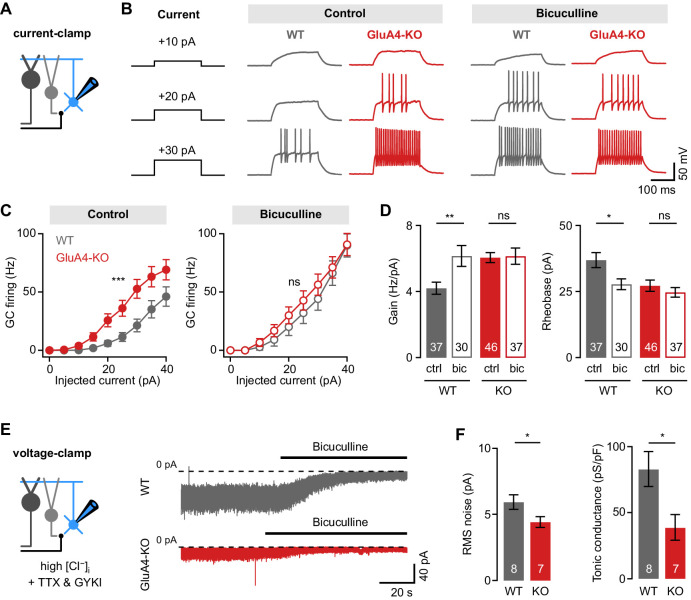
Figure 2. Reduced tonic inhibition increases the granule cell (GC) input-output relationship. (A) Current-clamp recordings from GCs. (B) Example responses to somatic current injection of indicated amplitude for control and in the presence of 10 µM bicuculline. (C) Average GC firing frequency plotted vs. injected current for wild type (WT) and knockout (KO) in control and bicuculline. (D) Average gain and rheobase, calculated from the frequency-current curves in (C). In the presence of bicuculline, KO GCs had gain and rheobase values comparable to WT. (E) Recording of tonic holding current. GABAergic currents were isolated using 20 µM GYKI-53655 and an intracellular solution with high [Cl−] to maximize GABAA receptor-mediated currents (see Materials and methods). Right: Example recordings of bicuculline wash-in (10 µM) for WT and KO GCs. (F) Average root-mean-square noise before wash-in of bicuculline (left; p = 0.048; d = −1.11) and average tonic conductance density (right; p = 0.020; d = −1.35) for WT and GluA4-KO. Tonic conductance was calculated from the bicuculline-sensitive current. Data are means ± SEM.
Figure 2. Reduced tonic inhibition increases the granule cell (GC) input-output relationship. (A) Current-clamp recordings from GCs. (B) Example responses to somatic current injection of indicated amplitude for control and in the presence of 10 µM bicuculline. (C) Average GC firing frequency plotted vs. injected current for wild type (WT) and knockout (KO) in control and bicuculline. (D) Average gain and rheobase, calculated from the frequency-current curves in (C). In the presence of bicuculline, KO GCs had gain and rheobase values comparable to WT. (E) Recording of tonic holding current. GABAergic currents were isolated using 20 µM GYKI-53655 and an intracellular solution with high [Cl−] to maximize GABAA receptor-mediated currents (see Materials and methods). Right: Example recordings of bicuculline wash-in (10 µM) for WT and KO GCs. (F) Average root-mean-square noise before wash-in of bicuculline (left; p = 0.048; d = −1.11) and average tonic conductance density (right; p = 0.020; d = −1.35) for WT and GluA4-KO. Tonic conductance was calculated from the bicuculline-sensitive current. Data are means ± SEM.CC BY · PubMed Central
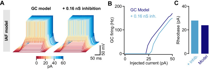
Figure 2—figure supplement 1. Tonic inhibition in a cerebellar granule cell (GC) integrate-and-fire model. (A) Membrane voltages of an integrate-and-fire (IAF) model in response to current injections of increasing amplitude (color coded). Adding 0.16 nS tonic inhibitory conductance reduces excitability. (B) Action potential firing frequency vs. injected current for the model with (light blue) and without (dark blue) tonic inhibition. (C) Rheobase current of the IAF model for both conditions.
Figure 2—figure supplement 1. Tonic inhibition in a cerebellar granule cell (GC) integrate-and-fire model. (A) Membrane voltages of an integrate-and-fire (IAF) model in response to current injections of increasing amplitude (color coded). Adding 0.16 nS tonic inhibitory conductance reduces excitability. (B) Action potential firing frequency vs. injected current for the model with (light blue) and without (dark blue) tonic inhibition. (C) Rheobase current of the IAF model for both conditions.CC BY · PubMed Central
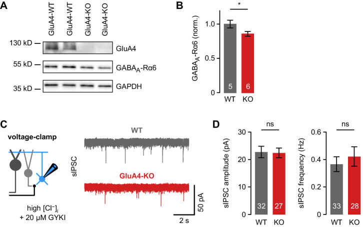
Figure 2—figure supplement 2. Phasic inhibition in cerebellar granule cells (GCs) of wild-type (WT) and GluA4-knockout (GluA4-KO) mice. (A) Western blot of cerebellar lysates from mice of indicated genotypes labeled for GluA4, α6 GABAA receptor (GABAAR) subunit (GABAA-Rα6), and GAPDH. (B) Normalized α6 GABAAR expression in WT and GluA4-KO (p = 0.028). Data are normalized to GAPDH and WT, and are averages of two to four technical and five to six biological replicates (per genotype). (C) Left: Spontaneous inhibitory postsynaptic current (sIPSC) recordings in GCs. Inhibitory currents were isolated using 20 µM GYKI-53655 and a CsCl-based intracellular solution. Right: Example sIPSC recordings from WT and GluA4-KO GCs. (D) Average sIPSC amplitude (left; p = 0.54) and frequency (right; p = 0.53) for WT and GluA4-KO. Data are means ± SEM.
Figure 2—figure supplement 2. Phasic inhibition in cerebellar granule cells (GCs) of wild-type (WT) and GluA4-knockout (GluA4-KO) mice. (A) Western blot of cerebellar lysates from mice of indicated genotypes labeled for GluA4, α6 GABAA receptor (GABAAR) subunit (GABAA-Rα6), and GAPDH. (B) Normalized α6 GABAAR expression in WT and GluA4-KO (p = 0.028). Data are normalized to GAPDH and WT, and are averages of two to four technical and five to six biological replicates (per genotype). (C) Left: Spontaneous inhibitory postsynaptic current (sIPSC) recordings in GCs. Inhibitory currents were isolated using 20 µM GYKI-53655 and a CsCl-based intracellular solution. Right: Example sIPSC recordings from WT and GluA4-KO GCs. (D) Average sIPSC amplitude (left; p = 0.54) and frequency (right; p = 0.53) for WT and GluA4-KO. Data are means ± SEM.CC BY · PubMed Central
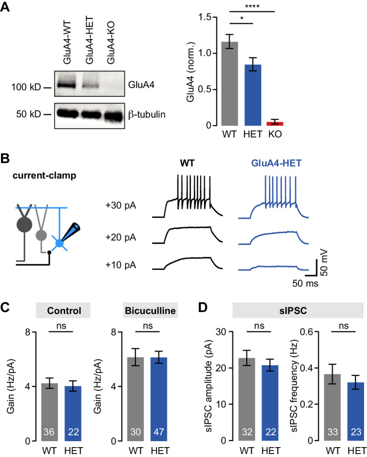
Figure 2—figure supplement 3. Normal tonic and phasic inhibition in heterozygous GluA4 (GluA4-HET) granule cells (GCs). (A) Left: Western blot of cerebellar lysates from indicated genotypes labeled for GluA4 and β-tubulin. Right: Normalized GluA4 expression in wild type (WT), GluA4-HET, and GluA4-knockout (GluA4-KO). Data are normalized to β-tubulin and are averages of three technical and five biological replicates (per genotype). (B) Example responses to somatic current injection of indicated amplitude for WT and GluA4-HET under control conditions. (C) Average gain of the frequency-current relationship for control (left; p = 0.77) and bicuculline (right; p = 0.22). (D) Average spontaneous inhibitory postsynaptic current (sIPSC) amplitude (left; p = 0.28) and frequency (right; p = 0.53) for WT and GluA4-HET. Data are means ± SEM.
Figure 2—figure supplement 3. Normal tonic and phasic inhibition in heterozygous GluA4 (GluA4-HET) granule cells (GCs). (A) Left: Western blot of cerebellar lysates from indicated genotypes labeled for GluA4 and β-tubulin. Right: Normalized GluA4 expression in wild type (WT), GluA4-HET, and GluA4-knockout (GluA4-KO). Data are normalized to β-tubulin and are averages of three technical and five biological replicates (per genotype). (B) Example responses to somatic current injection of indicated amplitude for WT and GluA4-HET under control conditions. (C) Average gain of the frequency-current relationship for control (left; p = 0.77) and bicuculline (right; p = 0.22). (D) Average spontaneous inhibitory postsynaptic current (sIPSC) amplitude (left; p = 0.28) and frequency (right; p = 0.53) for WT and GluA4-HET. Data are means ± SEM.CC BY · PubMed Central
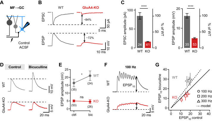
Figure 3. Shunting inhibition controls excitatory postsynaptic potential (EPSP) size in cerebellar granule cells (GCs). (A) Recordings from mossy fiber (MF)→GC connections in voltage- or current-clamp with blocker-free artificial cerebrospinal fluid (ACSF) (‘control’). (B) Example excitatory postsynaptic current (EPSC) and excitatory postsynaptic potential (EPSP) recordings from the same cell in wild type (WT) and knockout (KO). Arrows indicate reduction compared to WT. (C) Average EPSC (left, p < 0.0001, d = −2.62) and EPSP amplitudes (right, p < 0.0001, d = −2.37) for WT and KO. Note the difference in relative reduction of EPSPs compared to EPSCs. (D) Example EPSP recordings for control and in the presence of 10 µM bicuculline. (E) Average EPSP amplitude for WT and KO. Error bars represent 95% CI. (F) Example MF→GC EPSP trains (10 stimuli, 100 Hz). (G) Average EPSP10 in the presence of bicuculline vs. control for the indicated stimulation frequencies. Black line represents unity and dashed line the prediction of an integrate-and-fire model with or without tonic inhibition (Figure 2—figure supplement 1). Data in (C) and (G) are means ± SEM.
Figure 3. Shunting inhibition controls excitatory postsynaptic potential (EPSP) size in cerebellar granule cells (GCs). (A) Recordings from mossy fiber (MF)→GC connections in voltage- or current-clamp with blocker-free artificial cerebrospinal fluid (ACSF) (‘control’). (B) Example excitatory postsynaptic current (EPSC) and excitatory postsynaptic potential (EPSP) recordings from the same cell in wild type (WT) and knockout (KO). Arrows indicate reduction compared to WT. (C) Average EPSC (left, p < 0.0001, d = −2.62) and EPSP amplitudes (right, p < 0.0001, d = −2.37) for WT and KO. Note the difference in relative reduction of EPSPs compared to EPSCs. (D) Example EPSP recordings for control and in the presence of 10 µM bicuculline. (E) Average EPSP amplitude for WT and KO. Error bars represent 95% CI. (F) Example MF→GC EPSP trains (10 stimuli, 100 Hz). (G) Average EPSP10 in the presence of bicuculline vs. control for the indicated stimulation frequencies. Black line represents unity and dashed line the prediction of an integrate-and-fire model with or without tonic inhibition (Figure 2—figure supplement 1). Data in (C) and (G) are means ± SEM.CC BY · PubMed Central
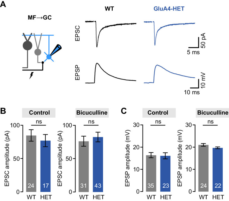
Figure 3—figure supplement 1. Normal mossy fiber (MF)→granule cell (GC) excitatory postsynaptic currents (EPSCs) and excitatory postsynaptic potentials (EPSPs) in heterozygous GluA4 (GluA4-HET) GCs. (A) Example EPSCs and EPSPs for wild type (WT) and GluA4-HET under control conditions. (B) Average EPSC amplitude for WT and GluA4-HET for control and bicuculline. Bicuculline data are redrawn from Delvendahl et al., 2019. (C) Average EPSP amplitude for WT and GluA4-HET. Note that EPSPs were larger in both genotypes in the presence of bicuculline. Data are means ± SEM. n.s. p > 0.05.
Figure 3—figure supplement 1. Normal mossy fiber (MF)→granule cell (GC) excitatory postsynaptic currents (EPSCs) and excitatory postsynaptic potentials (EPSPs) in heterozygous GluA4 (GluA4-HET) GCs. (A) Example EPSCs and EPSPs for wild type (WT) and GluA4-HET under control conditions. (B) Average EPSC amplitude for WT and GluA4-HET for control and bicuculline. Bicuculline data are redrawn from Delvendahl et al., 2019. (C) Average EPSP amplitude for WT and GluA4-HET. Note that EPSPs were larger in both genotypes in the presence of bicuculline. Data are means ± SEM. n.s. p > 0.05.CC BY · PubMed Central
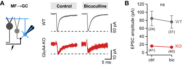
Figure 3—figure supplement 2. Similar mossy fiber (MF)→granule cell (GC) excitatory postsynaptic current (EPSC) amplitudes between control and bicuculline. (A) Example MF→GC EPSCs in wild-type (WT) and GluA4-knockout (GluA4-KO) GCs for control and bicuculline. (B) Average EPSC amplitude of WT and GluA4-KO was not different between control (‘ctrl’) and bicuculline (‘bic’) (ANOVA drug × genotype: F = 0.35, p = 0.56, η2p = 0.003). Data are means ± 95% confidence interval.
Figure 3—figure supplement 2. Similar mossy fiber (MF)→granule cell (GC) excitatory postsynaptic current (EPSC) amplitudes between control and bicuculline. (A) Example MF→GC EPSCs in wild-type (WT) and GluA4-knockout (GluA4-KO) GCs for control and bicuculline. (B) Average EPSC amplitude of WT and GluA4-KO was not different between control (‘ctrl’) and bicuculline (‘bic’) (ANOVA drug × genotype: F = 0.35, p = 0.56, η2p = 0.003). Data are means ± 95% confidence interval.CC BY · PubMed Central
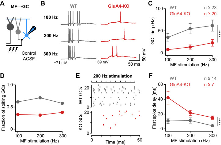
Figure 4. Deletion of GluA4 impairs granule cell (GC) spike fidelity and precision during high-frequency transmission. (A) Recordings from mossy fiber (MF)→GC connections in current-clamp. GCs were held at −70 mV. (B) Example voltage recordings from a wild type (WT) and GluA4-knockout (GluA4-KO) GC upon MF stimulation with 10 stimuli at increasing frequencies (indicated). (C) Average GC firing frequency upon MF stimulation with 100–300 Hz frequency. (D) Fraction of GCs showing spikes upon 100–300 Hz MF stimulation. (E) Spike raster plots for 200 Hz MF stimulation in WT and GluA4-KO. (F) Average first spike delay calculated from stimulation onset plotted vs. MF stimulation frequency. Data are means ± SEM.
Figure 4. Deletion of GluA4 impairs granule cell (GC) spike fidelity and precision during high-frequency transmission. (A) Recordings from mossy fiber (MF)→GC connections in current-clamp. GCs were held at −70 mV. (B) Example voltage recordings from a wild type (WT) and GluA4-knockout (GluA4-KO) GC upon MF stimulation with 10 stimuli at increasing frequencies (indicated). (C) Average GC firing frequency upon MF stimulation with 100–300 Hz frequency. (D) Fraction of GCs showing spikes upon 100–300 Hz MF stimulation. (E) Spike raster plots for 200 Hz MF stimulation in WT and GluA4-KO. (F) Average first spike delay calculated from stimulation onset plotted vs. MF stimulation frequency. Data are means ± SEM.CC BY · PubMed Central
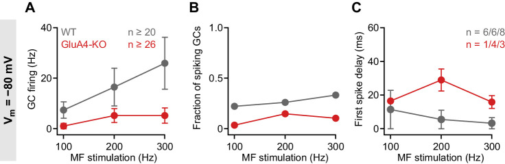
Figure 4—figure supplement 1. Impaired granule cell (GC) spike output in GluA4-knockout (GluA4-KO) GCs at −80 mV. (A) Average GC firing frequency upon mossy fiber (MF) stimulation with 100–300 Hz frequency for wild type (WT) and GluA4-KO. GC membrane voltage was maintained at −80 mV by current injection. (B) Fraction of GCs showing spikes upon MF stimulation with 100–300 Hz frequency. (C) Average first spike delay plotted vs. MF stimulation frequency; delay was calculated from stimulation onset. Data are means ± SEM.
Figure 4—figure supplement 1. Impaired granule cell (GC) spike output in GluA4-knockout (GluA4-KO) GCs at −80 mV. (A) Average GC firing frequency upon mossy fiber (MF) stimulation with 100–300 Hz frequency for wild type (WT) and GluA4-KO. GC membrane voltage was maintained at −80 mV by current injection. (B) Fraction of GCs showing spikes upon MF stimulation with 100–300 Hz frequency. (C) Average first spike delay plotted vs. MF stimulation frequency; delay was calculated from stimulation onset. Data are means ± SEM.CC BY · PubMed Central
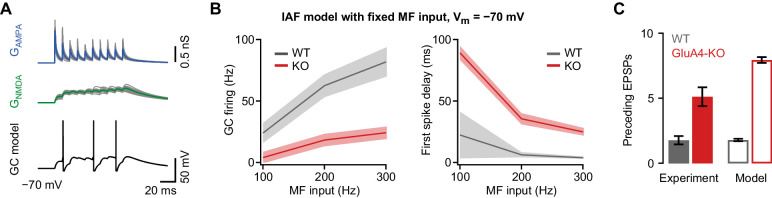
Figure 4—figure supplement 2. Impaired granule cell (GC) spiking in an integrate-and-fire (IAF) GC model. (A) Top: Simulated 100 Hz AMPA receptor (AMPAR) (GAMPA, blue) and NMDA receptor (NMDAR) conductances (GNMDA, green) using a binomial model of short-term plasticity (20 individual traces in gray overlaid with averages in color). Bottom: Result of single simulation using a GC IAF model (black; Figure 2—figure supplement 1) with wild-type (WT) GAMPA and GNMDA. (B) Left: Average model firing frequency upon mossy fiber (MF) input with 100–300 Hz frequency. The model included either WT or GluA4-knockout (GluA4-KO) synaptic conductances as indicated. Right: Average first spike delay calculated from stimulation onset plotted vs. MF stimulation frequency. Data are means, shadows represent SD. (C) Average number of excitatory postsynaptic potentials (EPSPs) preceding the first GC spike for WT and GluA4-KO (300 Hz MF stimulation) together with corresponding results from simulation. Data are means ± SEM.
Figure 4—figure supplement 2. Impaired granule cell (GC) spiking in an integrate-and-fire (IAF) GC model. (A) Top: Simulated 100 Hz AMPA receptor (AMPAR) (GAMPA, blue) and NMDA receptor (NMDAR) conductances (GNMDA, green) using a binomial model of short-term plasticity (20 individual traces in gray overlaid with averages in color). Bottom: Result of single simulation using a GC IAF model (black; Figure 2—figure supplement 1) with wild-type (WT) GAMPA and GNMDA. (B) Left: Average model firing frequency upon mossy fiber (MF) input with 100–300 Hz frequency. The model included either WT or GluA4-knockout (GluA4-KO) synaptic conductances as indicated. Right: Average first spike delay calculated from stimulation onset plotted vs. MF stimulation frequency. Data are means, shadows represent SD. (C) Average number of excitatory postsynaptic potentials (EPSPs) preceding the first GC spike for WT and GluA4-KO (300 Hz MF stimulation) together with corresponding results from simulation. Data are means ± SEM.CC BY · PubMed Central
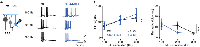
Figure 4—figure supplement 3. Normal granule cell (GC) spike output in heterozygous GluA4 (GluA4-HET) GCs. (A) Example voltage recordings from a wild-type (WT) and GluA4-HET GC upon mossy fiber (MF) stimulation with 10 stimuli at increasing frequencies (indicated). GC membrane voltage was maintained at −70mV. (B) Left: Average GC firing frequency upon MF stimulation with 100–300 Hz frequency (ANOVA genotype: F = 0.22, p = 0.64, η2p = 0.002). Right: Average first spike delay (calculated from stimulation onset) plotted vs. MF stimulation frequency. Data are means ± SEM. n.s. p > 0.05.
Figure 4—figure supplement 3. Normal granule cell (GC) spike output in heterozygous GluA4 (GluA4-HET) GCs. (A) Example voltage recordings from a wild-type (WT) and GluA4-HET GC upon mossy fiber (MF) stimulation with 10 stimuli at increasing frequencies (indicated). GC membrane voltage was maintained at −70mV. (B) Left: Average GC firing frequency upon MF stimulation with 100–300 Hz frequency (ANOVA genotype: F = 0.22, p = 0.64, η2p = 0.002). Right: Average first spike delay (calculated from stimulation onset) plotted vs. MF stimulation frequency. Data are means ± SEM. n.s. p > 0.05.CC BY · PubMed Central
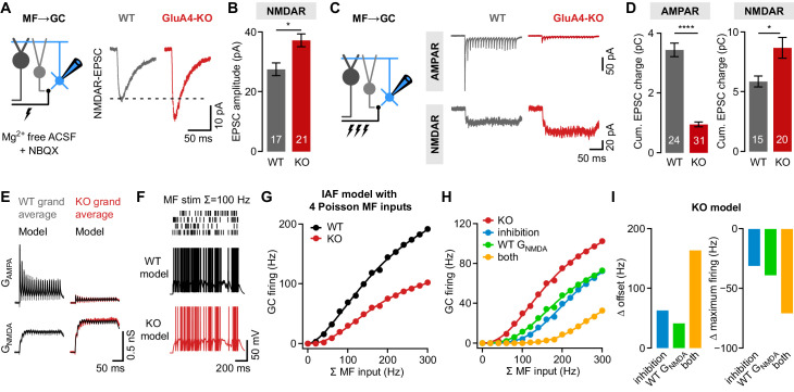
Figure 5. NMDA receptors (NMDARs) and reduced inhibition support spiking in GluA4-knockout (GluA4-KO) granule cells (GCs). (A) Left: Recordings of isolated NMDAR-EPSCs (excitatory postsynaptic currents) at mossy fiber (MF)→GC connections. Right: Example NMDAR-mediated MF→GC EPSCs. (B) Average EPSC amplitude for wild-type (WT) and GluA4-KO GCs (p = 0.0026; d = 1.04). (C) Left: Schematic of MF→GC train stimulation. Top: Example AMPA receptor (AMPAR)-EPSC 100 Hz train recordings (20 stimuli) for WT and KO. Bottom: Example NMDAR-mediated 100 Hz trains. (D) Average cumulative charge for AMPAR-mediated (left; p < 0.0001; d = −3.05) and NMDAR-mediated EPSCs (right; p = 0.0063; d = 0.92) for both genotypes. (E) Grand average of AMPAR and NMDAR conductance trains (20 stimuli, 100 Hz) recorded from WT (left) and GluA4-KO GCs (right). Data are overlaid with synaptic conductance models for WT and GluA4-KO. (F) Top: Four independent Poisson-distributed MF spike trains with a sum of 100 Hz (top) and simulation results for WT (black) and KO (red). (G) Average WT and KO model firing frequency vs. MF stimulation frequency. Lines are fits with a Hill equation. (H) Results for KO model compared with simulations of KO GCs with tonic inhibition (blue), with WT GNMDA (green) or both (yellow). (I) Reduced inhibition and enhanced GNMDA reduce the offset (left) and increase the maximum firing frequency (right) of the KO model GC output. Data are means ± SEM.
Figure 5. NMDA receptors (NMDARs) and reduced inhibition support spiking in GluA4-knockout (GluA4-KO) granule cells (GCs). (A) Left: Recordings of isolated NMDAR-EPSCs (excitatory postsynaptic currents) at mossy fiber (MF)→GC connections. Right: Example NMDAR-mediated MF→GC EPSCs. (B) Average EPSC amplitude for wild-type (WT) and GluA4-KO GCs (p = 0.0026; d = 1.04). (C) Left: Schematic of MF→GC train stimulation. Top: Example AMPA receptor (AMPAR)-EPSC 100 Hz train recordings (20 stimuli) for WT and KO. Bottom: Example NMDAR-mediated 100 Hz trains. (D) Average cumulative charge for AMPAR-mediated (left; p < 0.0001; d = −3.05) and NMDAR-mediated EPSCs (right; p = 0.0063; d = 0.92) for both genotypes. (E) Grand average of AMPAR and NMDAR conductance trains (20 stimuli, 100 Hz) recorded from WT (left) and GluA4-KO GCs (right). Data are overlaid with synaptic conductance models for WT and GluA4-KO. (F) Top: Four independent Poisson-distributed MF spike trains with a sum of 100 Hz (top) and simulation results for WT (black) and KO (red). (G) Average WT and KO model firing frequency vs. MF stimulation frequency. Lines are fits with a Hill equation. (H) Results for KO model compared with simulations of KO GCs with tonic inhibition (blue), with WT GNMDA (green) or both (yellow). (I) Reduced inhibition and enhanced GNMDA reduce the offset (left) and increase the maximum firing frequency (right) of the KO model GC output. Data are means ± SEM.CC BY · PubMed Central
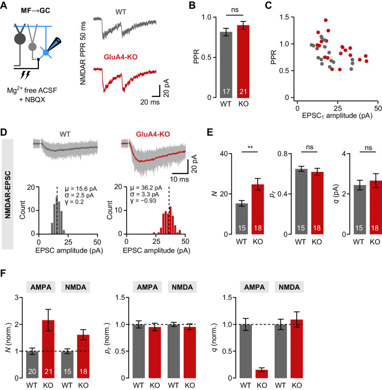
Figure 5—figure supplement 1. Increased number of presynaptic release sites in GluA4-knockout (GluA4-KO) mice. (A) Example mossy fiber (MF)→granule cell (GC) paired-pulses at 50 ms inter-stimulus interval. NMDA receptor (NMDAR)-mediated excitatory postsynaptic currents (EPSCs) were isolated using 10 µM NBQX and 0 mM external Mg2+. (B) Average paired-pulse ratio (PPR) for wild-type (WT) and GluA4-KO GCs (p = 0.23). (C) NMDAR-PPR vs. amplitude of the first EPSC (EPSC1). (D) Top: Example NMDAR-EPSC recordings. Shown are 60 individual sweeps overlaid with the average. Bottom: Histogram of EPSC amplitudes for the examples shown above. Mean (μ), standard deviation (σ), and skewness (γ) are indicated. (E) Quantification of the number of release sites (N; p = 0.0064, d = 0.98), release probability (pr; p = 0.50, d = −0.23), and quantal size (q; p = 0.60, d = 0.18) for WT and GluA4-KO. Statistical moments analysis of quanta (‘SMAQ’, Holler et al., 2021) was used to estimate binomial parameters from NMDAR-EPSCs. (F) Normalized SMAQ-derived N, pr, and q for AMPAR- and NMDAR-mediated EPSCs (normalized to WT). Data are means ± SEM.
Figure 5—figure supplement 1. Increased number of presynaptic release sites in GluA4-knockout (GluA4-KO) mice. (A) Example mossy fiber (MF)→granule cell (GC) paired-pulses at 50 ms inter-stimulus interval. NMDA receptor (NMDAR)-mediated excitatory postsynaptic currents (EPSCs) were isolated using 10 µM NBQX and 0 mM external Mg2+. (B) Average paired-pulse ratio (PPR) for wild-type (WT) and GluA4-KO GCs (p = 0.23). (C) NMDAR-PPR vs. amplitude of the first EPSC (EPSC1). (D) Top: Example NMDAR-EPSC recordings. Shown are 60 individual sweeps overlaid with the average. Bottom: Histogram of EPSC amplitudes for the examples shown above. Mean (μ), standard deviation (σ), and skewness (γ) are indicated. (E) Quantification of the number of release sites (N; p = 0.0064, d = 0.98), release probability (pr; p = 0.50, d = −0.23), and quantal size (q; p = 0.60, d = 0.18) for WT and GluA4-KO. Statistical moments analysis of quanta (‘SMAQ’, Holler et al., 2021) was used to estimate binomial parameters from NMDAR-EPSCs. (F) Normalized SMAQ-derived N, pr, and q for AMPAR- and NMDAR-mediated EPSCs (normalized to WT). Data are means ± SEM.CC BY · PubMed Central
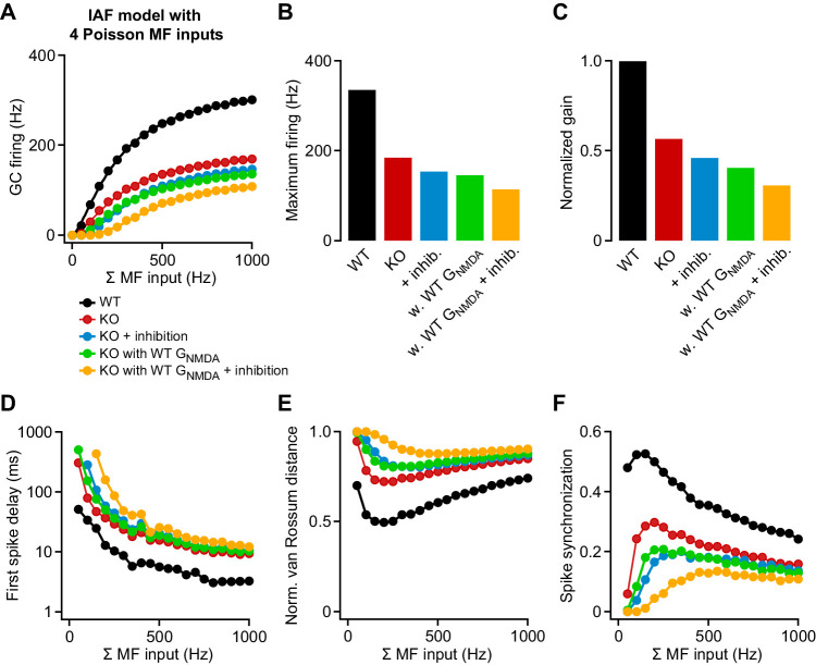
Figure 5—figure supplement 2. Contribution of attenuated inhibition and enhanced GNMDA to granule cell (GC) spike output. (A) Average wild-type (WT) and knockout (KO) model firing frequency vs. mossy fiber (MF) input frequency for a range of 50–1000 Hz. Lines are fits with a Hill equation (see Materials and methods). (B) Maximum firing frequency determined from fits to the data in (A). (C) Gain of the input-output relation, normalized to the WT simulation. (D) Average first spike delay vs. MF input frequency. Note the log scale of the ordinate. (E) Normalized van Rossum distance vs. MF input frequency. The van Rossum distance was calculated using an exponential kernel with τ = 10 ms, and normalized to the maximum error for each frequency (calculated for all random MF spike trains without postsynaptic spikes). (F) Spike synchronization (see Materials and methods) vs. MF input frequency of 50–1000 Hz. Larger values indicate higher synchrony of pre- and postsynaptic spikes.
Figure 5—figure supplement 2. Contribution of attenuated inhibition and enhanced GNMDA to granule cell (GC) spike output. (A) Average wild-type (WT) and knockout (KO) model firing frequency vs. mossy fiber (MF) input frequency for a range of 50–1000 Hz. Lines are fits with a Hill equation (see Materials and methods). (B) Maximum firing frequency determined from fits to the data in (A). (C) Gain of the input-output relation, normalized to the WT simulation. (D) Average first spike delay vs. MF input frequency. Note the log scale of the ordinate. (E) Normalized van Rossum distance vs. MF input frequency. The van Rossum distance was calculated using an exponential kernel with τ = 10 ms, and normalized to the maximum error for each frequency (calculated for all random MF spike trains without postsynaptic spikes). (F) Spike synchronization (see Materials and methods) vs. MF input frequency of 50–1000 Hz. Larger values indicate higher synchrony of pre- and postsynaptic spikes.CC BY · PubMed Central
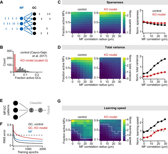
Figure 6. Impaired pattern separation in a feedforward model of the cerebellar input layer. (A) Schematic of the feedforward network model. The model comprises 187 mossy fibers (MFs) that are connected to 487 granule cells (GCs) with four synapses per GC. The network is presented with different MF activity patterns, which produce GC spike patterns. (B) Histogram of active GCs. Scaling synaptic (AMPA receptor [AMPAR] and NMDA receptor [NMDAR]) conductance and tonic inhibitory conductance according to the GluA4-knockout (GluA4-KO) data (‘KO model’, red) leads to strong reduction of active GCs compared to the model from Cayco-Gajic et al., 2017 (‘control’, black). (C) Left: Normalized population sparseness (normalized to MF sparseness) plotted for different MF correlation radii and fraction of active MFs of both models. Right: Median normalized sparseness vs. MF correlation radius. Median is calculated across fractions of active MFs. (D) Same as (C), but for total variance. (E) Schematic of learning implementation. MF or GC activity patterns are used to train a perceptron decoder to classify these patterns into 10 random classes. (F) Root-mean-square (RMS) error of the perceptron classification for MF input patterns (blue), GC input patterns (black) or GC patterns with scaled conductance (red). Dashed line indicates cutoff for learning speed quantification. (G) Left: Normalized learning speed (normalized to learning using MF patterns) plotted for different MF correlation radii and fraction of active MFs of both models. White dashed borders indicate areas of faster learning with GC activity patterns than with MF patterns. Right: Median normalized learning speed vs. MF correlation radius. Dashed line indicates faster GC learning.
Figure 6. Impaired pattern separation in a feedforward model of the cerebellar input layer. (A) Schematic of the feedforward network model. The model comprises 187 mossy fibers (MFs) that are connected to 487 granule cells (GCs) with four synapses per GC. The network is presented with different MF activity patterns, which produce GC spike patterns. (B) Histogram of active GCs. Scaling synaptic (AMPA receptor [AMPAR] and NMDA receptor [NMDAR]) conductance and tonic inhibitory conductance according to the GluA4-knockout (GluA4-KO) data (‘KO model’, red) leads to strong reduction of active GCs compared to the model from Cayco-Gajic et al., 2017 (‘control’, black). (C) Left: Normalized population sparseness (normalized to MF sparseness) plotted for different MF correlation radii and fraction of active MFs of both models. Right: Median normalized sparseness vs. MF correlation radius. Median is calculated across fractions of active MFs. (D) Same as (C), but for total variance. (E) Schematic of learning implementation. MF or GC activity patterns are used to train a perceptron decoder to classify these patterns into 10 random classes. (F) Root-mean-square (RMS) error of the perceptron classification for MF input patterns (blue), GC input patterns (black) or GC patterns with scaled conductance (red). Dashed line indicates cutoff for learning speed quantification. (G) Left: Normalized learning speed (normalized to learning using MF patterns) plotted for different MF correlation radii and fraction of active MFs of both models. White dashed borders indicate areas of faster learning with GC activity patterns than with MF patterns. Right: Median normalized learning speed vs. MF correlation radius. Dashed line indicates faster GC learning.CC BY · PubMed Central
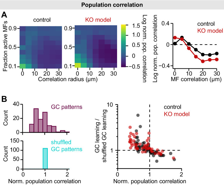
Figure 6—figure supplement 1. Population correlations in the mossy fiber (MF)-granule cell (GC) feedforward model. (A) Left: Log-normalized population correlation (see Materials and methods; normalized to MF correlations) plotted for different MF correlation radii and fraction of active MFs of both models. Right: Median log-normalized population correlation vs. MF correlation radius. Data points below dashed line indicate active decorrelation. Median is calculated across fractions of active MFs. (B) To assess the contribution of decorrelation to learning speed, we used shuffled GC patterns to train the perceptron (Cayco-Gajic et al., 2017). GC patterns were shuffled to achieve the same population correlation as MF patterns, while preserving sparseness and total variance. Left: Histograms of normalized GC population correlation before and after shuffling. Right: The contribution of decorrelation to learning speed is similar in both models. GC learning speed is normalized to speed using shuffled patterns and plotted vs. population correlation.
Figure 6—figure supplement 1. Population correlations in the mossy fiber (MF)-granule cell (GC) feedforward model. (A) Left: Log-normalized population correlation (see Materials and methods; normalized to MF correlations) plotted for different MF correlation radii and fraction of active MFs of both models. Right: Median log-normalized population correlation vs. MF correlation radius. Data points below dashed line indicate active decorrelation. Median is calculated across fractions of active MFs. (B) To assess the contribution of decorrelation to learning speed, we used shuffled GC patterns to train the perceptron (Cayco-Gajic et al., 2017). GC patterns were shuffled to achieve the same population correlation as MF patterns, while preserving sparseness and total variance. Left: Histograms of normalized GC population correlation before and after shuffling. Right: The contribution of decorrelation to learning speed is similar in both models. GC learning speed is normalized to speed using shuffled patterns and plotted vs. population correlation.CC BY · PubMed Central
Figure 7. Normal locomotor coordination of GluA4-knockout (GluA4-KO) mice during overground walking. (A) LocoMouse apparatus. (B) Continuous tracks (in x, y, z) for nose, paws, and tail segments obtained from LocoMouse tracking (Machado et al., 2015) are plotted on top of the frame. (C) Individual strides were divided into swing and stance phases for further analysis. (D)–(E) Stride length of front right (FR) paw (D) and hind right (HR) paw (E) vs. walking speed for GluA4-KO mice (red) and wild-type (WT) animals (gray). For each parameter, the thin lines with shadows represent median values ± 25th, 75th percentiles. (F)–(G) Average instantaneous forward (x) velocity of FR paw (F) and HR paw (G) during swing phase. (H)–(I) Average vertical (z) position of FR paw (H) and HR paw (I) relative to ground during swing. The shaded area indicates SEM across mice. (J)–(K) Polar plots indicating the phase of the step cycle in which each limb enters stance, aligned to stance onset of FR paw (red circle). Distance from the origin represents walking speed. (J) WT mice; (K) GluA4-KO mice. Circles show average values for each animal.
Figure 7. Normal locomotor coordination of GluA4-knockout (GluA4-KO) mice during overground walking. (A) LocoMouse apparatus. (B) Continuous tracks (in x, y, z) for nose, paws, and tail segments obtained from LocoMouse tracking (Machado et al., 2015) are plotted on top of the frame. (C) Individual strides were divided into swing and stance phases for further analysis. (D)–(E) Stride length of front right (FR) paw (D) and hind right (HR) paw (E) vs. walking speed for GluA4-KO mice (red) and wild-type (WT) animals (gray). For each parameter, the thin lines with shadows represent median values ± 25th, 75th percentiles. (F)–(G) Average instantaneous forward (x) velocity of FR paw (F) and HR paw (G) during swing phase. (H)–(I) Average vertical (z) position of FR paw (H) and HR paw (I) relative to ground during swing. The shaded area indicates SEM across mice. (J)–(K) Polar plots indicating the phase of the step cycle in which each limb enters stance, aligned to stance onset of FR paw (red circle). Distance from the origin represents walking speed. (J) WT mice; (K) GluA4-KO mice. Circles show average values for each animal.CC BY · PubMed Central
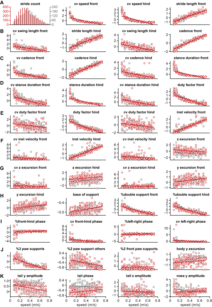
Figure 7—figure supplement 1. Distribution of z-scored values for all gait parameters. Each circle represents the mean z-scored value of that gait parameter for one animal at one speed bin. Wild-type ( WT) animals are in gray and GluA4-knockout (GluA4-KO) animals in red. Lines are linear fits of each parameter for each animal group, across speed bins. Raw data for individual limb parameters (rows (A) to (H)). Interlimb parameters across speed bins (rows (H) to (J)). Whole body gait parameters over speed (last panel (J) and row (K)). Definitions of each parameter and method for calculating it are given in the Materials and methods section.
Figure 7—figure supplement 1. Distribution of z-scored values for all gait parameters. Each circle represents the mean z-scored value of that gait parameter for one animal at one speed bin. Wild-type ( WT) animals are in gray and GluA4-knockout (GluA4-KO) animals in red. Lines are linear fits of each parameter for each animal group, across speed bins. Raw data for individual limb parameters (rows (A) to (H)). Interlimb parameters across speed bins (rows (H) to (J)). Whole body gait parameters over speed (last panel (J) and row (K)). Definitions of each parameter and method for calculating it are given in the Materials and methods section.CC BY · PubMed Central
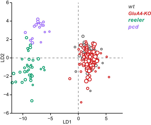
Figure 7—figure supplement 2. Linear discriminant analysis separates ataxic mutants from GluA4-knockout (GluA4-KO) and control animals. Linear discriminant analysis of locomotor kinematics reveals two axes, which separate ataxic mutants from GluA4-KO and control (WT) animals (LD1) and from each other (LD2). The gait measurements from Figure 7—figure supplement 1 comprised the inputs to the LDA (see Materials and methods). Each circle represents a single animal walking at a particular speed. Faster speeds are shown with larger marker sizes. Speeds ranged from 0.05 to 0.8 m/s and were binned with a binwidth of 0.05 m/s. Size-matched controls for GluA4-KO animals are in gray (N = 9 for all speed bins), GluA4-KO animals are in red (N = 12 for all speed bins), reeler in green (N = 7 for 0.05–0.15 m/s; N = 6 for 0.25–0.35 m/s; n = ~2387), and pcd in purple (N = 3 for all speed bins except 0.25–0.30 m/s N = 2; n = ~3066). Reeler and pcd data are from Machado et al., 2015 and Machado et al., 2020a.
Figure 7—figure supplement 2. Linear discriminant analysis separates ataxic mutants from GluA4-knockout (GluA4-KO) and control animals. Linear discriminant analysis of locomotor kinematics reveals two axes, which separate ataxic mutants from GluA4-KO and control (WT) animals (LD1) and from each other (LD2). The gait measurements from Figure 7—figure supplement 1 comprised the inputs to the LDA (see Materials and methods). Each circle represents a single animal walking at a particular speed. Faster speeds are shown with larger marker sizes. Speeds ranged from 0.05 to 0.8 m/s and were binned with a binwidth of 0.05 m/s. Size-matched controls for GluA4-KO animals are in gray (N = 9 for all speed bins), GluA4-KO animals are in red (N = 12 for all speed bins), reeler in green (N = 7 for 0.05–0.15 m/s; N = 6 for 0.25–0.35 m/s; n = ~2387), and pcd in purple (N = 3 for all speed bins except 0.25–0.30 m/s N = 2; n = ~3066). Reeler and pcd data are from Machado et al., 2015 and Machado et al., 2020a.CC BY · PubMed Central
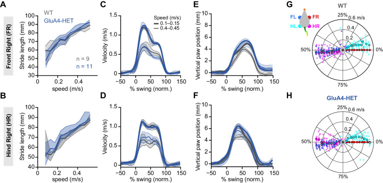
Figure 7—figure supplement 3. Normal locomotion in heterozygous GluA4 (GluA4-HET) mice. (A)–(B) Stride length of front right (FR) paw (A) and hind right (HR) paw (B) vs. walking speed for GluA4-HET mice (blue) and wild-type (WT) animals (gray). For each parameter, the thin lines with shadows represent median values ± 25th, 75th percentiles. (C)–(D) Average instantaneous forward (x) velocity of FR paw (C) and HR paw (D) during swing phase. (E)–(F) Average vertical (z) position of FR paw (E) and HR paw (F) relative to ground during swing. The shaded area indicates SEM across mice. (G)–(H) Polar plots indicating the phase of the step cycle in which each limb enters stance, aligned to stance onset of FR paw (red circle). Distance from the origin represents walking speed. (G) WT mice; (H) GluA4-HET mice. Circles show average values for each animal.
Figure 7—figure supplement 3. Normal locomotion in heterozygous GluA4 (GluA4-HET) mice. (A)–(B) Stride length of front right (FR) paw (A) and hind right (HR) paw (B) vs. walking speed for GluA4-HET mice (blue) and wild-type (WT) animals (gray). For each parameter, the thin lines with shadows represent median values ± 25th, 75th percentiles. (C)–(D) Average instantaneous forward (x) velocity of FR paw (C) and HR paw (D) during swing phase. (E)–(F) Average vertical (z) position of FR paw (E) and HR paw (F) relative to ground during swing. The shaded area indicates SEM across mice. (G)–(H) Polar plots indicating the phase of the step cycle in which each limb enters stance, aligned to stance onset of FR paw (red circle). Distance from the origin represents walking speed. (G) WT mice; (H) GluA4-HET mice. Circles show average values for each animal.CC BY · PubMed Central
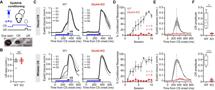
Figure 8. GluA4 is required for cerebellum-dependent associative memory formation. (A) Top: Schematic of the eyeblink conditioning paradigm, where a conditioned stimulus (CS) (a white LED or a whisker vibratory stimulus) is repeatedly paired and co-terminates with an eyeblink-eliciting unconditioned stimulus (US) (a puff of air delivered to the eye). Bottom: Example video frames (acquired at 900 fps under infrared light) illustrate automated extraction of eyelid movement amplitude. (B) Normalized mean unconditioned response area for wild type (WT) and GluA4-knockout (GluA4-KO) (WT: n = 12; KO: n = 9; p = 0.36). (C) Average eyelid closure across nine learning sessions (S1–S9) of representative WT and KO animals, using a visual CS (top) or a whisker CS (bottom). Each trace represents the average of 100 paired trials from a single session. (D) Average %CR (% conditioned response) learning curves of WT (gray) and GluA4-KO (red) mice trained with either a visual CS (top) or a whisker CS (bottom). Error bars indicate SEM. (E) Average eyelid traces of CS-only trials from the last training session of WT and GluA4-KO animals, trained with either a visual CS (top) or a whisker CS (bottom). Shadows indicate SEM. Vertical dashed line represents the time that the US would have been expected on CS+US trials. (F) Average CR amplitudes from the last training session of WT and GluA4-KO animals, trained with either a visual CS (top; p = 0.0029) or a whisker CS (bottom; p < 0.0001). Box indicates median and 25th–75th percentiles; whiskers extend to the most extreme data points.
Figure 8. GluA4 is required for cerebellum-dependent associative memory formation. (A) Top: Schematic of the eyeblink conditioning paradigm, where a conditioned stimulus (CS) (a white LED or a whisker vibratory stimulus) is repeatedly paired and co-terminates with an eyeblink-eliciting unconditioned stimulus (US) (a puff of air delivered to the eye). Bottom: Example video frames (acquired at 900 fps under infrared light) illustrate automated extraction of eyelid movement amplitude. (B) Normalized mean unconditioned response area for wild type (WT) and GluA4-knockout (GluA4-KO) (WT: n = 12; KO: n = 9; p = 0.36). (C) Average eyelid closure across nine learning sessions (S1–S9) of representative WT and KO animals, using a visual CS (top) or a whisker CS (bottom). Each trace represents the average of 100 paired trials from a single session. (D) Average %CR (% conditioned response) learning curves of WT (gray) and GluA4-KO (red) mice trained with either a visual CS (top) or a whisker CS (bottom). Error bars indicate SEM. (E) Average eyelid traces of CS-only trials from the last training session of WT and GluA4-KO animals, trained with either a visual CS (top) or a whisker CS (bottom). Shadows indicate SEM. Vertical dashed line represents the time that the US would have been expected on CS+US trials. (F) Average CR amplitudes from the last training session of WT and GluA4-KO animals, trained with either a visual CS (top; p = 0.0029) or a whisker CS (bottom; p < 0.0001). Box indicates median and 25th–75th percentiles; whiskers extend to the most extreme data points.CC BY · PubMed Central
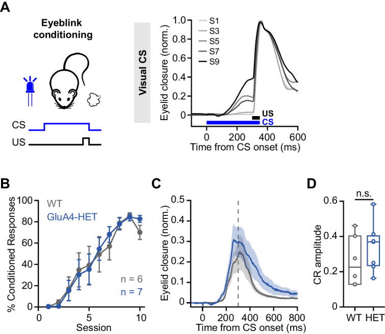
Figure 8—figure supplement 1. Normal associative learning in heterozygous GluA4 (GluA4-HET) mice. (A) Left: Schematic of eyeblink conditioning experiment. Right: Average eyelid closure across nine learning sessions (S1–S9) of a representative wild-type (WT) animal using a visual conditioned stimulus (CS). Each trace represents the average of 100 paired trials from a single session. (B) Average %CR (% conditioned response) learning curves of WT (gray) and GluA4-HET (blue) mice. Error bars indicate SEM. (C) Average eyelid traces of CS-only trials from the last training session of WT and GluA4-HET animals. Shadows indicate SEM. Vertical dashed line represents the time that the unconditioned stimulus (US) would have been expected on CS+US trials. (D) Average CR amplitudes from the last training session of WT and GluA4-HET animals. Box indicates median and 25th–75th percentiles; whiskers extend to the most extreme data points. n.s. p > 0.05.
Figure 8—figure supplement 1. Normal associative learning in heterozygous GluA4 (GluA4-HET) mice. (A) Left: Schematic of eyeblink conditioning experiment. Right: Average eyelid closure across nine learning sessions (S1–S9) of a representative wild-type (WT) animal using a visual conditioned stimulus (CS). Each trace represents the average of 100 paired trials from a single session. (B) Average %CR (% conditioned response) learning curves of WT (gray) and GluA4-HET (blue) mice. Error bars indicate SEM. (C) Average eyelid traces of CS-only trials from the last training session of WT and GluA4-HET animals. Shadows indicate SEM. Vertical dashed line represents the time that the unconditioned stimulus (US) would have been expected on CS+US trials. (D) Average CR amplitudes from the last training session of WT and GluA4-HET animals. Box indicates median and 25th–75th percentiles; whiskers extend to the most extreme data points. n.s. p > 0.05.CC BY · PubMed Central

Verification

Claims the paper makes

The claims and statistics of this paper haven’t been checked yet.

Run the check — free, no account needed. It reads the open-access text and checks the sources it cites.

A few free checks a day · papers already verified open instantly · results are public

Claims other papers make about this one

Each is checked against this paper’s own text: does it say what the citing paper says it does?

Self-check

Percentages, sums and reported differences re-computed from the paper’s own numbers.

The self-check needs the paper’s full text.

Citations

Cites

Research works printed but not linked: 102

  1. Aizenman, 2000, Rapid, synaptically driven increases in the intrinsic excitability of cerebellar deep nuclear neurons, Nature Neuroscience, 3, 109, 10.1038/72049 · DOI
  2. Albergaria, 2018, Locomotor activity modulates associative learning in mouse cerebellum, Nature Neuroscience, 21, 725, 10.1038/s41593-018-0129-x · DOI
  3. Andreescu, 2011, NR2A subunit of the N-methyl d-aspartate receptors are required for potentiation at the mossy fiber to granule cell synapse and vestibulo-cerebellar motor learning, Neuroscience, 176, 274, 10.1016/j.neuroscience.2010.12.024 · DOI
  4. Arenz, 2008, The contribution of single synapses to sensory representation in vivo, Science, 321, 977, 10.1126/science.1158391 · DOI
  5. Bates, 2015, Fitting linear mixed-effects models using lme4, Journal of Statistical Software, 67, 1, 10.18637/jss.v067.i01 · DOI · Paper page
  6. Billings, 2014, Network structure within the cerebellar input layer enables lossless sparse encoding, Neuron, 83, 960, 10.1016/j.neuron.2014.07.020 · DOI
  7. Brette, 2005, Adaptive exponential integrate-and-fire model as an effective description of neuronal activity, Journal of Neurophysiology, 94, 3637, 10.1152/jn.00686.2005 · DOI
  8. Brickley, 2001, Adaptive regulation of neuronal excitability by a voltage-independent potassium conductance, Nature, 409, 88, 10.1038/35051086 · DOI
  9. Carey, 2011, Synaptic mechanisms of sensorimotor learning in the cerebellum, Current Opinion in Neurobiology, 21, 609, 10.1016/j.conb.2011.06.011 · DOI
  10. Cathala, 2005, Changes in synaptic structure underlie the developmental speeding of AMPA receptor-mediated EPSCs, Nature Neuroscience, 8, 1310, 10.1038/nn1534 · DOI
  11. Cayco-Gajic, 2017, Sparse synaptic connectivity is required for decorrelation and pattern separation in feedforward networks, Nature Communications, 8, 10.1038/s41467-017-01109-y · DOI
  12. Cayco-Gajic, 2019, Re-evaluating circuit mechanisms underlying pattern separation, Neuron, 101, 584, 10.1016/j.neuron.2019.01.044 · DOI
  13. Chadderton, 2004, Integration of quanta in cerebellar granule cells during sensory processing, Nature, 428, 856, 10.1038/nature02442 · DOI
  14. Chen, 1999, Impaired cerebellar synapse maturation in Waggler, a mutant mouse with a disrupted neuronal calcium channel gamma subunit, PNAS, 96, 12132, 10.1073/pnas.96.21.12132 · DOI
  15. Chourbaji, 2008, AMPA receptor subunit 1 (GluR-A) knockout mice model the glutamate hypothesis of depression, FASEB Journal, 22, 3129, 10.1096/fj.08-106450 · DOI · Paper page
  16. Citri, 2010, Calcium binding to PICK1 is essential for the intracellular retention of AMPA receptors underlying long-term depression, Journal of Neuroscience, 30, 16437, 10.1523/JNEUROSCI.4478-10.2010 · DOI
  17. D'Angelo, 1995, Synaptic excitation of individual rat cerebellar granule cells in situ: evidence for the role of NMDA receptors, The Journal of Physiology, 484, 397, 10.1113/jphysiol.1995.sp020673 · DOI
  18. D'Angelo, 2009, Timing and plasticity in the cerebellum: focus on the granular layer, Trends in Neurosciences, 32, 30, 10.1016/j.tins.2008.09.007 · DOI
  19. De Zeeuw, 2005, Time and tide in cerebellar memory formation, Current Opinion in Neurobiology, 15, 667, 10.1016/j.conb.2005.10.008 · DOI
  20. Delvendahl, 2015, Dendritic patch-clamp recordings from cerebellar granule cells demonstrate electrotonic compactness, Frontiers in Cellular Neuroscience, 9, 10.3389/fncel.2015.00093 · DOI
  21. Delvendahl, 2019, Rapid and sustained homeostatic control of presynaptic exocytosis at a central synapse, PNAS, 116, 23783, 10.1073/pnas.1909675116 · DOI
  22. Delvendahl I. 2021. GluA4_cerebellum_eLife. Software Heritage. swh:1:rev:1d1c19853e18f8fbb3307eeecc64096e53d74820. https://archive.softwareheritage.org/swh:1:dir:ed0f67ce39e290326cfdfaa541af7b1603e8b863;origin=https://github.com/delvendahl/GluA4_cerebellum_eLife;visit=swh:1:snp:e6beee2411b3fe4b998787a69ed26b8a6f1fb734;anchor=swh:1:rev:1d1c19853e18f8fbb3307eeecc64096e53d74820.
  23. Delvendahl, 2016, The cerebellar mossy fiber synapse as a model for high-frequency transmission in the mammalian CNS, Trends in Neurosciences, 39, 722, 10.1016/j.tins.2016.09.006 · DOI · Paper page
  24. Desai, 1999, Plasticity in the intrinsic excitability of cortical pyramidal neurons, Nature Neuroscience, 2, 515, 10.1038/9165 · DOI · Paper page
  25. Dieudonné, 1995, Glycinergic synaptic currents in Golgi cells of the rat cerebellum, PNAS, 92, 1441, 10.1073/pnas.92.5.1441 · DOI
  26. DiGregorio, 2002, Spillover of glutamate onto synaptic AMPA receptors enhances fast transmission at a cerebellar synapse, Neuron, 35, 521, 10.1016/S0896-6273(02)00787-0 · DOI
  27. Duguid, 2012, Tonic inhibition enhances fidelity of sensory information transmission in the cerebellar cortex, Journal of Neuroscience, 32, 11132, 10.1523/JNEUROSCI.0460-12.2012 · DOI
  28. Duguid, 2015, Control of cerebellar granule cell output by sensory-evoked Golgi cell inhibition, PNAS, 112, 13099, 10.1073/pnas.1510249112 · DOI
  29. Freeman, 2011, Neural circuitry and plasticity mechanisms underlying delay eyeblink conditioning, Learning & Memory, 18, 666, 10.1101/lm.2023011 · DOI · Paper page
  30. Fuchs, 2007, Recruitment of parvalbumin-positive interneurons determines hippocampal function and associated behavior, Neuron, 53, 591, 10.1016/j.neuron.2007.01.031 · DOI · Paper page
  31. Gall, 2003, Altered neuronal excitability in cerebellar granule cells of mice lacking calretinin, The Journal of Neuroscience, 23, 9320, 10.1523/JNEUROSCI.23-28-09320.2003 · DOI
  32. Galliano, 2013, Silencing the majority of cerebellar granule cells uncovers their essential role in motor learning and consolidation, Cell Reports, 3, 1239, 10.1016/j.celrep.2013.03.023 · DOI
  33. Geiger, 1995, Relative abundance of subunit mRNAs determines gating and Ca2+ permeability of AMPA receptors in principal neurons and interneurons in rat CNS, Neuron, 15, 193, 10.1016/0896-6273(95)90076-4 · DOI · Paper page
  34. Giovannucci, 2017, Cerebellar granule cells acquire a widespread predictive feedback signal during motor learning, Nature Neuroscience, 20, 727, 10.1038/nn.4531 · DOI
  35. Grasselli, 2020, SK2 channels in cerebellar Purkinje cells contribute to excitability modulation in motor-learning-specific memory traces, PLOS Biology, 18, 10.1371/journal.pbio.3000596 · DOI
  36. Gründer, 2000, Distribution and developmental regulation of AMPA receptor subunit proteins in rat retina, Investigative Ophthalmology & Visual Science, 41, 3600
  37. Hadzic, 2017, Ionotropic glutamate receptors: which ones, when, and where in the mammalian neocortex, Journal of Comparative Neurology, 525, 976, 10.1002/cne.24103 · DOI · Paper page
  38. Hamann, 2002, Tonic and spillover inhibition of granule cells control information flow through cerebellar cortex, Neuron, 33, 625, 10.1016/S0896-6273(02)00593-7 · DOI
  39. Hashimoto, 1999, Impairment of AMPA receptor function in cerebellar granule cells of ataxic mutant mouse stargazer, The Journal of Neuroscience, 19, 6027, 10.1523/JNEUROSCI.19-14-06027.1999 · DOI
  40. Heck, 2013, The neuronal code(s) of the cerebellum, Journal of Neuroscience, 33, 17603, 10.1523/JNEUROSCI.2759-13.2013 · DOI
  41. Heiney, 2014, Cerebellar-dependent expression of motor learning during eyeblink conditioning in head-fixed mice, Journal of Neuroscience, 34, 14845, 10.1523/JNEUROSCI.2820-14.2014 · DOI
  42. Hollmann, 1994, Cloned glutamate receptors, Annual Review of Neuroscience, 17, 31, 10.1146/annurev.ne.17.030194.000335 · DOI
  43. Huupponen, 2016, GluA4 subunit of AMPA receptors mediates the early synaptic response to altered network activity in the developing hippocampus, Journal of Neurophysiology, 115, 2989, 10.1152/jn.00435.2015 · DOI
  44. Ishikawa, 2015, Multimodal sensory integration in single cerebellar granule cells in vivo, eLife, 4, 10.7554/eLife.12916 · DOI
  45. Jackson, 2011, Stargazin (TARP γ-2) is required for compartment-specific AMPA receptor trafficking and synaptic plasticity in cerebellar stellate cells, Journal of Neuroscience, 31, 3939, 10.1523/JNEUROSCI.5134-10.2011 · DOI
  46. Kanichay, 2008, Synaptic and cellular properties of the feedforward inhibitory circuit within the input layer of the cerebellar cortex, Journal of Neuroscience, 28, 8955, 10.1523/JNEUROSCI.5469-07.2008 · DOI
  47. Karmarkar, 2006, Different forms of homeostatic plasticity are engaged with distinct temporal profiles: differential expression of homeostatic plasticity, European Journal of Neuroscience, 23, 1575, 10.1111/j.1460-9568.2006.04692.x · DOI
  48. Keinänen, 1990, A family of AMPA-selective glutamate receptors, Science, 249, 556, 10.1126/science.2166337 · DOI · Paper page
  49. Knogler, 2017, Sensorimotor representations in cerebellar granule cells in larval zebrafish are dense, spatially organized, and non-temporally patterned, Current Biology, 27, 1288, 10.1016/j.cub.2017.03.029 · DOI
  50. Lambolez, 1992, AMPA receptor subunits expressed by single Purkinje cells, Neuron, 9, 247, 10.1016/0896-6273(92)90164-9 · DOI
  51. Lanore, 2021, Cerebellar granule cell axons support high-dimensional representations, Nature Neuroscience, 10, 10.1038/s41593-021-00873-x · DOI
  52. Machado, 2015, A quantitative framework for whole-body coordination reveals specific deficits in freely walking ataxic mice, eLife, 4, 10.7554/eLife.07892 · DOI
  53. Machado, 2020, Shared and specific signatures of locomotor ataxia in mutant mice, eLife, 9, 10.7554/eLife.55356 · DOI
  54. Markwalter, 2019, Sensorimotor coding of vermal granule neurons in the developing mammalian cerebellum, The Journal of Neuroscience, 39, 6626, 10.1523/JNEUROSCI.0086-19.2019 · DOI
  55. Marr, 1969, A theory of cerebellar cortex, The Journal of Physiology, 202, 437, 10.1113/jphysiol.1969.sp008820 · DOI · Paper page
  56. Mauk, 1997, Roles of cerebellar cortex and nuclei in motor learning: contradictions or clues?, Neuron, 18, 343, 10.1016/S0896-6273(00)81235-0 · DOI
  57. McCormick, 1984, Cerebellum: essential involvement in the classically conditioned eyelid response, Science, 223, 296, 10.1126/science.6701513 · DOI
  58. Mitchell, 2003, Shunting inhibition modulates neuronal gain during synaptic excitation, Neuron, 38, 433, 10.1016/S0896-6273(03)00200-9 · DOI · Paper page
  59. Monyer, 1991, Glutamate-operated channels: developmentally early and mature forms arise by alternative splicing, Neuron, 6, 799, 10.1016/0896-6273(91)90176-Z · DOI · Paper page
  60. Morton, 2007, Mechanisms of cerebellar gait ataxia, The Cerebellum, 6, 79, 10.1080/14734220601187741 · DOI
  61. Mosbacher, 1994, A molecular determinant for submillisecond desensitization in glutamate receptors, Science, 266, 1059, 10.1126/science.7973663 · DOI
  62. Mulansky, 2016, PySpike—A Python library for analyzing spike train synchrony, SoftwareX, 5, 183, 10.1016/j.softx.2016.07.006 · DOI
  63. Muzzu, 2018, Encoding of locomotion kinematics in the mouse cerebellum, PLOS ONE, 13, 10.1371/journal.pone.0203900 · DOI
  64. Osborne, 2007, Time course of precision in smooth-pursuit eye movements of monkeys, Journal of Neuroscience, 27, 2987, 10.1523/JNEUROSCI.5072-06.2007 · DOI
  65. Payne, 2007, GABAA α6-containing receptors are selectively compromised in cerebellar granule cells of the ataxic mouse, stargazer, Journal of Biological Chemistry, 282, 29130, 10.1074/jbc.M700111200 · DOI
  66. Paz, 2011, A new mode of corticothalamic transmission revealed in the Gria4(-/-) model of absence epilepsy, Nature Neuroscience, 14, 1167, 10.1038/nn.2896 · DOI
  67. Peter, 2020, AMPAR auxiliary protein SHISA6 facilitates Purkinje cell synaptic excitability and procedural memory formation, Cell Reports, 31, 10.1016/j.celrep.2020.03.079 · DOI
  68. Powell, 2015, Synaptic representation of locomotion in single cerebellar granule cells, eLife, 4, 10.7554/eLife.07290 · DOI
  69. Qin, 1999, AMPA-selective glutamate receptor subunits GluR2 and GluR4 in the cat retina: an immunocytochemical study, Visual Neuroscience, 16, 1105, 10.1017/S0952523899166100 · DOI
  70. Rancz, 2007, High-fidelity transmission of sensory information by single cerebellar mossy fibre boutons, Nature, 450, 1245, 10.1038/nature05995 · DOI
  71. Raymond, 2018, Computational principles of supervised learning in the cerebellum, Annual Review of Neuroscience, 41, 233, 10.1146/annurev-neuro-080317-061948 · DOI
  72. Ritzau-Jost, 2014, Ultrafast action potentials mediate kilohertz signaling at a central synapse, Neuron, 84, 152, 10.1016/j.neuron.2014.08.036 · DOI
  73. Rizwan, 2016, Long-term potentiation at the mossy fiber-granule cell relay invokes postsynaptic second-messenger regulation of Kv4 channels, The Journal of Neuroscience, 36, 11196, 10.1523/JNEUROSCI.2051-16.2016 · DOI
  74. Roth, 2020, Cortical synaptic AMPA receptor plasticity during motor learning, Neuron, 105, 895, 10.1016/j.neuron.2019.12.005 · DOI
  75. Rothman, 2009, Synaptic depression enables neuronal gain control, Nature, 457, 1015, 10.1038/nature07604 · DOI
  76. Rothman, 2014, Data-driven modeling of synaptic transmission and integration, Prog Mol Biol Transl Sci., 123, 305, 10.1016/B978-0-12-397897-4.00004-8 · DOI
  77. Rothman, 2018, NeuroMatic: an integrated open-source software toolkit for acquisition, analysis and simulation of electrophysiological data, Frontiers in Neuroinformatics, 12, 10.3389/fninf.2018.00014 · DOI
  78. Rudolph, 2020, Cerebellum-specific deletion of the GABAA receptor δ subunit leads to sex-specific disruption of behavior, Cell Reports, 33, 10.1016/j.celrep.2020.108338 · DOI
  79. Saab, 2012, Bergmann glial AMPA receptors are required for fine motor coordination, Science, 337, 749, 10.1126/science.1221140 · DOI
  80. Schweighofer, 2001, Unsupervised learning of granule cell sparse codes enhances cerebellar adaptive control, Neuroscience, 103, 35, 10.1016/S0306-4522(00)00548-0 · DOI
  81. Schwenk, 2014, Regional diversity and developmental dynamics of the AMPA-receptor proteome in the mammalian brain, Neuron, 84, 41, 10.1016/j.neuron.2014.08.044 · DOI
  82. Seja, 2012, Raising cytosolic Cl − in cerebellar granule cells affects their excitability and vestibulo-ocular learning, The EMBO Journal, 31, 1217, 10.1038/emboj.2011.488 · DOI
  83. Seol, 2015, Ionotropic glutamate receptor GluA4 and T-type calcium channel Cav3.1 subunits control key aspects of synaptic transmission at the mouse L5B-POm giant synapse, European Journal of Neuroscience, 42, 3033, 10.1111/ejn.13084 · DOI
  84. Shi, 2001, Subunit-specific rules governing AMPA receptor trafficking to synapses in hippocampal pyramidal neurons, Cell, 105, 331, 10.1016/S0092-8674(01)00321-X · DOI · Paper page
  85. Shimuta, 2020, Multiple signals evoked by unisensory stimulation converge onto cerebellar granule and Purkinje cells in mice, Communications Biology, 3, 10.1038/s42003-020-1110-2 · DOI
  86. Silva, 2019, MicroRNA-186-5p controls GluA2 surface expression and synaptic scaling in hippocampal neurons, PNAS, 116, 5727, 10.1073/pnas.1900338116 · DOI
  87. Soda, 2019, Hyperexcitability and hyperplasticity disrupt cerebellar signal transfer in the IB2 KO mouse model of autism, The Journal of Neuroscience, 39, 2383, 10.1523/JNEUROSCI.1985-18.2019 · DOI
  88. Stell, 2003, Neuroactive steroids reduce neuronal excitability by selectively enhancing tonic inhibition mediated by δ subunit-containing GABAA receptors, PNAS, 100, 14439, 10.1073/pnas.2435457100 · DOI
  89. Straub, 2020, Gradients in the mammalian cerebellar cortex enable Fourier-like transformation and improve storing capacity, eLife, 9, 10.7554/eLife.51771 · DOI
  90. Suvrathan, 2018, Depressed by learning—heterogeneity of the plasticity rules at parallel fiber synapses onto Purkinje cells, The Cerebellum, 17, 747, 10.1007/s12311-018-0968-8 · DOI
  91. Swanson, 1997, Single-channel properties of recombinant AMPA receptors depend on RNA editing, splice variation, and subunit composition, The Journal of Neuroscience, 17, 58, 10.1523/JNEUROSCI.17-01-00058.1997 · DOI
  92. Traynelis, 2010, Glutamate receptor ion channels: structure, regulation, and function, Pharmacological Reviews, 62, 405, 10.1124/pr.109.002451 · DOI · Paper page
  93. van Kan, 1993, Movement-related inputs to intermediate cerebellum of the monkey, Journal of Neurophysiology, 69, 74, 10.1152/jn.1993.69.1.74 · DOI
  94. Wada, 2007, Conditioned eyeblink learning is formed and stored without cerebellar granule cell transmission, PNAS, 104, 16690, 10.1073/pnas.0708165104 · DOI
  95. Witter, 2015, Regional functionality of the cerebellum, Current Opinion in Neurobiology, 33, 150, 10.1016/j.conb.2015.03.017 · DOI
  96. Yamasaki, 2011, Glutamate receptor δ2 is essential for input pathway-dependent regulation of synaptic AMPAR contents in cerebellar Purkinje cells, Journal of Neuroscience, 31, 3362, 10.1523/JNEUROSCI.5601-10.2011 · DOI
  97. Yan, 2013, Homeostatic control of synaptic transmission by distinct glutamate receptors, Neuron, 78, 687, 10.1016/j.neuron.2013.02.031 · DOI
  98. Yang, 2011, GluA4 is indispensable for driving fast neurotransmission across a high-fidelity central synapse, The Journal of Physiology, 589, 4209, 10.1113/jphysiol.2011.208066 · DOI
  99. Zamanillo, 1999, Importance of AMPA receptors for hippocampal synaptic plasticity but not for spatial learning, Science, 284, 1805, 10.1126/science.284.5421.1805 · DOI · Paper page
  100. Zhang, 2020, NMDARs contribute to the facial stimuli-evoked mossy fiber-granule cell synaptic transmission in vivo in mice, Neuroscience Letters, 736, 10.1016/j.neulet.2020.135285 · DOI
  101. Zhao, 2019, Architecture and subunit arrangement of native AMPA receptors elucidated by cryo-EM, Science, 364, 355, 10.1126/science.aaw8250 · DOI
  102. Zhu, 2000, Postnatal synaptic potentiation: delivery of GluR4-containing AMPA receptors by spontaneous activity, Nature Neuroscience, 3, 1098, 10.1038/80614 · DOI · Paper page

Cited by

Sorted by citations

See all 33

Metadata

Authors
Kita, K., Albergaria, C., Machado, A. S., Carey, M. R., Müller, M., & Delvendahl, I.
Affiliations
  • Department of Molecular Life Sciences, University of Zurich, Zurich, Switzerland
  • Champalimaud Neuroscience Programme, Champalimaud Centre for the Unknown, Lisbon, Portugal
Venue
eLife
Published
2021-07-05
Volume
10
ISSN
2050-084X
Cited by
33
References
9
Language
en
Funders
  • European Research Council (640093, 679881)
  • Fundação para a Ciência e a Tecnologia (PTDC/MED-NEU/30890/2017)
  • Swiss National Science Foundation (PP00P3_144816, PZ00P3_174018)

About these checks

Registry, retraction, Cites and statistics results are computed, not judged, with one exception: a printed reference that no index lists is read once by a model before it counts as a citation error. Claims are extracted by a model and kept only when their quote appears verbatim in the text; each cited source is then checked, with a model’s help, for whether it says what the claim relies on. Those verdicts can be wrong — read the claim’s quote and the cited source before relying on one.

Statistics and arithmetic are recomputed, not judged.

Confidence bands are shown only for fields calibrated on our annotated test set. None is calibrated yet, so no band is shown.

What counts as a claim ›How we measure confidence ›How we check this ›

Are you an author, or do you see a problem with this page? Request a review