

The DOI matches its Crossref record; 65 of the 66 references it cites were found in a registry or an index.
Rapid protein stability prediction using deep learning representations
Open accessPublished version of a preprint
Abstract
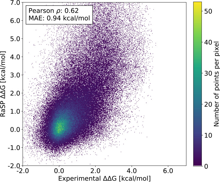
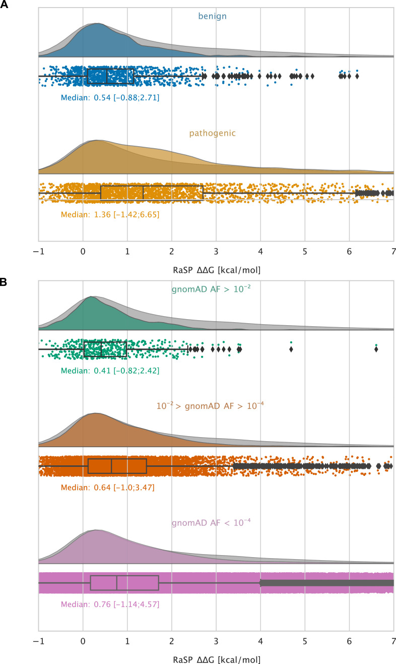
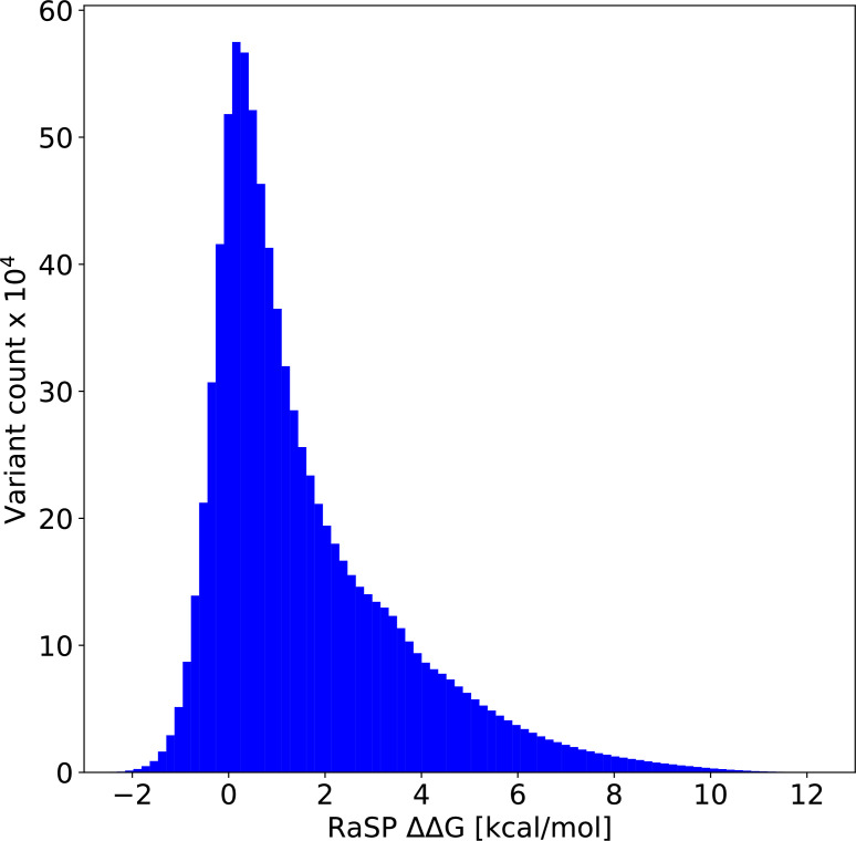
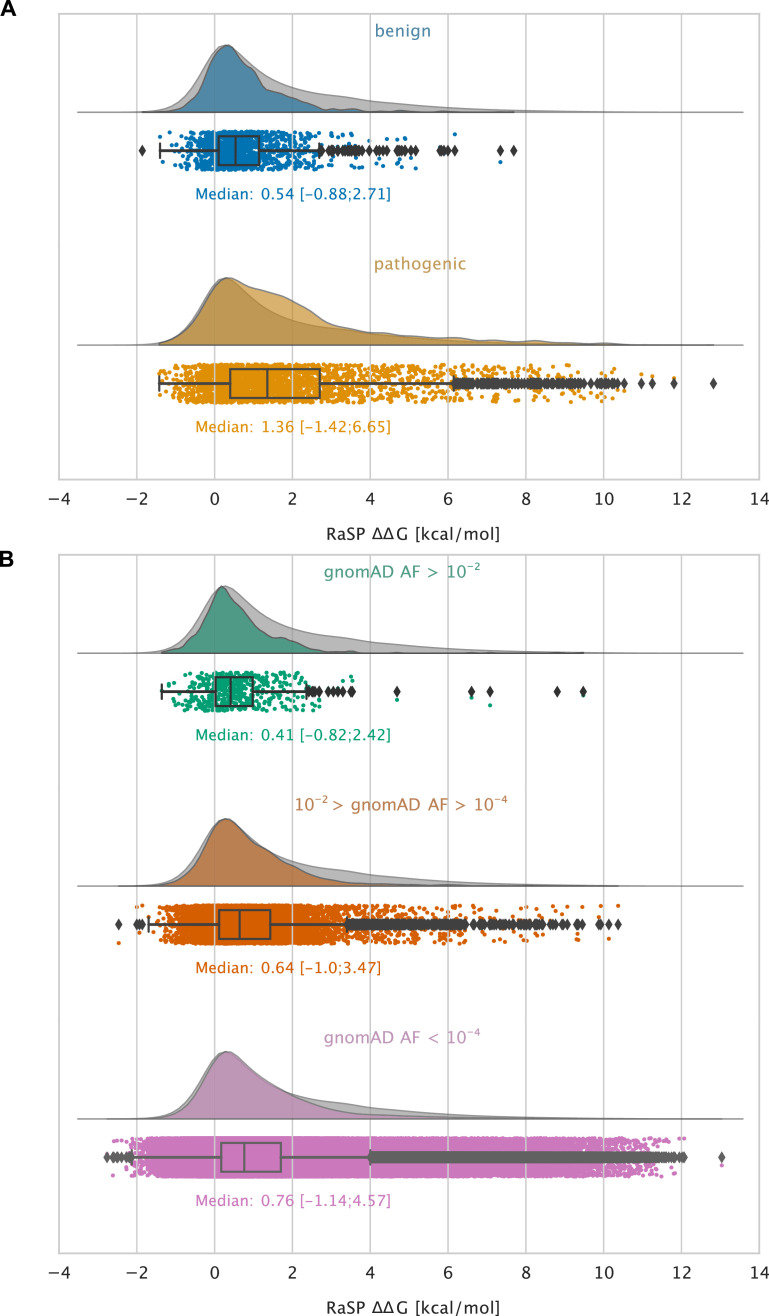
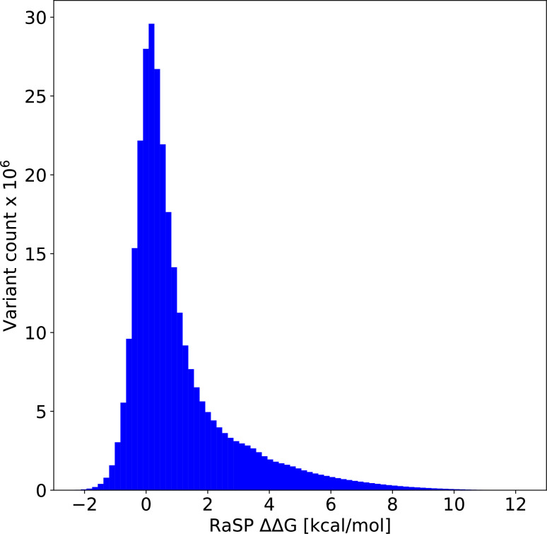
Predicting the thermodynamic stability of proteins is a common and widely used step in protein engineering, and when elucidating the molecular mechanisms behind evolution and disease. Here, we present RaSP, a method for making rapid and accurate predictions of changes in protein stability by leveraging deep learning representations. RaSP performs on-par with biophysics-based methods and enables saturation mutagenesis stability predictions in less than a second per residue. We use RaSP to calculate ∼ 230 million stability changes for nearly all single amino acid changes in the human proteome, and examine variants observed in the human population. We find that variants that are common in the population are substantially depleted for severe destabilization, and that there are substantial differences between benign and pathogenic variants, highlighting the role of protein stability in genetic diseases. RaSP is freely available—including via a Web interface—and enables large-scale analyses of stability in experimental and predicted protein structures.
Overview
The claims and statistics of this paper haven’t been checked yet.
Run the check — free, no account needed. It reads the open-access text and checks the sources it cites.
Integrity signals
Registry
Cites
Statistics
Figures
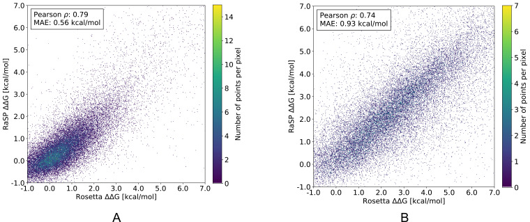
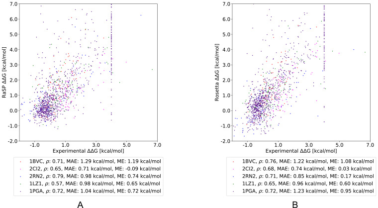
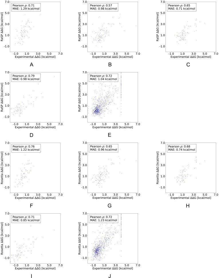
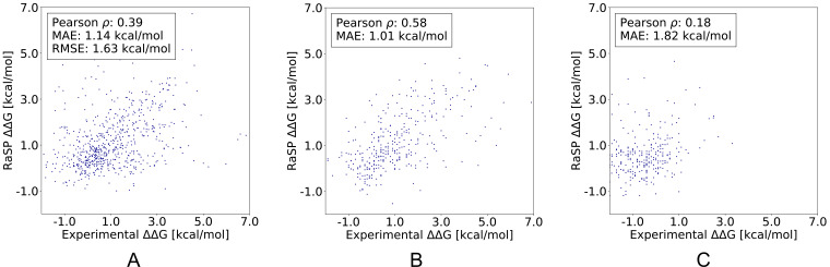
Verification
Claims the paper makes
The claims and statistics of this paper haven’t been checked yet.
Run the check — free, no account needed. It reads the open-access text and checks the sources it cites.
Self-check
Percentages, sums and reported differences re-computed from the paper’s own numbers.
The self-check needs the paper’s full text.
Citations
Cites
Adam: A Method for Stochastic Optimization
Kingma, D. P., & Ba, J. (2014) · arXiv · doi:10.48550/arxiv.1412.6980 · Cited by 98,946
Highly accurate protein structure prediction with AlphaFold
Jumper, J., Evans, R., Pritzel, A., Green, T., Figurnov, M., Ronneberger, O., Tunyasuvunakool, K., Bates, R., Žídek, A., Potapenko, A., et al. (2021) · Nature · doi:10.1038/s41586-021-03819-2 · Cited by 43,764
Gene Ontology: tool for the unification of biology
Ashburner, M., Ball, C. A., Blake, J. A., Botstein, D., Butler, H., Cherry, J. M., Davis, A. P., Dolinski, K., Dwight, S. S., Eppig, J. T., et al. (2000) · Nature Genetics · doi:10.1038/75556 · Cited by 43,206
Batch Normalization: Accelerating Deep Network Training by Reducing Internal Covariate Shift
Ioffe, S., & Szegedy, C. (2015) · arXiv · doi:10.48550/arxiv.1502.03167 · Cited by 27,818
Delving Deep into Rectifiers: Surpassing Human-Level Performance on ImageNet Classification
He, K., Zhang, X., Ren, S., & Sun, J. (2015) · 2015 IEEE International Conference on Computer Vision (ICCV) · doi:10.1109/iccv.2015.123 · Cited by 19,741
The mutational constraint spectrum quantified from variation in 141,456 humans
Karczewski, K. J., Francioli, L. C., Tiao, G., Cummings, B. B., Alföldi, J., Wang, Q., Collins, R. L., Laricchia, K. M., Ganna, A., Birnbaum, D. P., et al. (2020) · Nature · doi:10.1038/s41586-020-2308-7 · Cited by 9,434
Varadi, M., Anyango, S., Deshpande, M., Nair, S., Natassia, C., Yordanova, G., Yuan, D., Stroe, O., Wood, G., Laydon, A., et al. (2022) · Nucleic Acids Research · doi:10.1093/nar/gkab1061 · Cited by 7,850
Biopython: freely available python tools for computational molecular biology and bioinformatics
Cock, P. J. A., Antao, T., Chang, J. T., Chapman, B. A., Cox, C. J., Dalke, A., Friedberg, I., Hamelryck, T., Kauff, F., Wilczynski, B., et al. (2009) · Bioinformatics · doi:10.1093/bioinformatics/btp163 · Cited by 6,080
ClinVar: improving access to variant interpretations and supporting evidence
Landrum, M. J., Lee, J. M., Benson, M., Brown, G. R., Chao, C., Chitipiralla, S., Gu, B., Hart, J., Hoffman, D., Jang, W., et al. (2018) · Nucleic Acids Research · doi:10.1093/nar/gkx1153 · Cited by 4,196
Hierarchical models of object recognition in cortex
Riesenhuber, M., & Poggio, T. (1999) · Nature Neuroscience · doi:10.1038/14819 · Cited by 3,309
Research works printed but not linked: 1
- Linderstrøm-Lang Centre for Protein Science, University of Copenhagen. 2023. Rapid protein stability prediction using deep learning representations. Software Heritage. swh:1:rev:fb9438fa4724171e752fdf70e270db0cffc0f73c. https://archive.softwareheritage.org/swh:1:dir:3b5a5bf941013f41b9f7333e4190f4c9c4924cba;origin=https://github.com/KULL-Centre/_2022_ML-ddG-Blaabjerg;visit=swh:1:snp:2763a4dfde8edc3ee726a2aeb5897a90fc421c7c;anchor=swh:1:rev:fb9438fa4724171e752fdf70e270db0cffc0f73c.
Cited by
Sorted by citations
Machine learning for functional protein design
Notin, P., Rollins, N. J., Gal, Y., Sander, C., & Marks, D. S. (2024) · Nature Biotechnology · doi:10.1038/s41587-024-02127-0 · Cited by 304
Transfer learning to leverage larger datasets for improved prediction of protein stability changes
Dieckhaus, H., Brocidiacono, M., Randolph, N. Z., & Kuhlman, B. (2024) · Proceedings of the National Academy of Sciences · doi:10.1073/pnas.2314853121 · Cited by 205
Site-saturation mutagenesis of 500 human protein domains
Beltran, A., Jiang, X., Shen, Y., & Lehner, B. (2025) · Nature · doi:10.1038/s41586-024-08370-4 · Cited by 126
FireProt 2.0: web-based platform for the fully automated design of thermostable proteins
Musil, M., Jezik, A., Horackova, J., Borko, S., Kabourek, P., Damborský, J., & Bednář, D. (2023) · Briefings in Bioinformatics · doi:10.1093/bib/bbad425 · Cited by 113
Masters, M. R., Mahmoud, A. H., & Lill, M. A. (2025) · Nature Communications · doi:10.1038/s41467-025-63947-5 · Cited by 141
Koh, H. Y., Zheng, Y., Yang, M., Arora, R., Webb, G. I., Pan, S., Li, L., & Church, G. M. (2025) · Nature Reviews Bioengineering · doi:10.1038/s44222-025-00349-8 · Cited by 117
Discovering functionally important sites in proteins
Cagiada, M., Bottaro, S., Lindemose, S., Schenstrøm, S. M., Stein, A., Hartmann‐Petersen, R., & Lindorff‐Larsen, K. (2023) · Nature Communications · doi:10.1038/s41467-023-39909-0 · Cited by 89
Self-citationBiophysics-based protein language models for protein engineering
Gelman, S., Johnson, B., Freschlin, C. R., Sharma, A., D’Costa, S., Peters, J., Gitter, A., & Romero, P. A. (2025) · Nature Methods · doi:10.1038/s41592-025-02776-2 · Cited by 77
Diaz, D. J., Gong, C., Ouyang-Zhang, J., Loy, J. M., Wells, J., Yang, D. K., Ellington, A. D., Dimakis, A. G., & Klivans, A. R. (2024) · Nature Communications · doi:10.1038/s41467-024-49780-2 · Cited by 69
A mutational atlas for Parkin proteostasis
Clausen, L., Voutsinos, V., Cagiada, M., Johansson, K. E., Grønbæk-Thygesen, M., Nariya, S., Powell, R. L., Have, M. K. N., Oestergaard, V. H., Stein, A., et al. (2024) · Nature Communications · doi:10.1038/s41467-024-45829-4 · Cited by 51
Self-citationAn end-to-end framework for the prediction of protein structure and fitness from single sequence
Chen, Y., Xu, Y., Liu, D., Xing, Y., & Gong, H. (2024) · Nature Communications · doi:10.1038/s41467-024-51776-x · Cited by 45
Optimizing enzyme thermostability by combining multiple mutations using protein language model
Bian, J., Tan, P., Nie, T., Hong, L. Y., & Yang, G. (2024) · mLife · doi:10.1002/mlf2.12151 · Cited by 43
Gerasimavicius, L., Livesey, B. J., & Marsh, J. A. (2023) · Protein Science · doi:10.1002/pro.4688 · Cited by 41
Son, A., Park, J., Kim, W., Yoon, Y., Lee, S., Park, Y., & Kim, H. (2024) · Molecules · doi:10.3390/molecules29194626 · Cited by 42
Protein representations: Encoding biological information for machine learning in biocatalysis
Harding-Larsen, D., Funk, J., Madsen, N. G., Gharabli, H., Acevedo-Rocha, C. G., Mazurenko, S., & Welner, D. H. (2024) · Biotechnology Advances · doi:10.1016/j.biotechadv.2024.108459 · Cited by 38
Predicting absolute protein folding stability using generative models
Cagiada, M., Ovchinnikov, S., & Lindorff‐Larsen, K. (2024) · Protein Science · doi:10.1002/pro.5233 · Cited by 38
Self-citationGrønbæk-Thygesen, M., Voutsinos, V., Johansson, K. E., Schulze, T. K., Cagiada, M., Pedersen, L., Clausen, L., Nariya, S., Powell, R. L., Stein, A., et al. (2024) · Nature Communications · doi:10.1038/s41467-024-48481-0 · Cited by 38
Self-citationProtein stability prediction by fine-tuning a protein language model on a mega-scale dataset
Chu, S. K. S., Narang, K., & Siegel, J. B. (2024) · PLoS Computational Biology · doi:10.1371/journal.pcbi.1012248 · Cited by 39
Sun, J., Zhu, T., Cui, Y., & Wu, B. (2025) · The Innovation · doi:10.1016/j.xinn.2024.100750 · Cited by 45
Expert-guided protein language models enable accurate and blazingly fast fitness prediction
Marquet, C., Schlensok, J., Abakarova, M., Rost, B., & Laine, E. (2024) · Bioinformatics · doi:10.1093/bioinformatics/btae621 · Cited by 33
MutationExplorer : a webserver for mutation of proteins and 3D visualization of energetic impacts
Philipp, M., Moth, C. W., Ristic, N., Tiemann, J. K. S., Seufert, F., Panfilova, A., Meiler, J., Hildebrand, P. W., Stein, A., Wiegreffe, D., et al. (2024) · Nucleic Acids Research · doi:10.1093/nar/gkae301 · Cited by 35
Self-citationCarter, J. J., Walker, T. M., Walker, A. S., Whitfield, M. G., Morlock, G. P., Lynch, C. I., Adlard, D., Peto, T., Posey, J. E., Crook, D. W., et al. (2024) · JAC-Antimicrobial Resistance · doi:10.1093/jacamr/dlae037 · Cited by 32
Nourbakhsh, M., Degn, K., Saksager, A. B., Tiberti, M., & Papaleo, E. (2023) · Briefings in Bioinformatics · doi:10.1093/bib/bbad519 · Cited by 33
Decoding molecular mechanisms for loss-of-function variants in the human proteomePreprint
Cagiada, M., Jonsson, N., & Lindorff‐Larsen, K. (2024) · bioRxiv (Cold Spring Harbor Laboratory) · doi:10.1101/2024.05.21.595203 · Cited by 34
Self-citationPredicted mechanistic impacts of human protein missense variantsPreprint
Jänes, J., Müller, M., Selvaraj, S., Manoel, D., Stephenson, J. D., Gonçalves, C. I., Lafita, A., Polacco, B. J., Obernier, K., Alasoo, K., et al. (2024) · bioRxiv (Cold Spring Harbor Laboratory) · doi:10.1101/2024.05.29.596373 · Cited by 27
Prediction of Quality-control Degradation Signals in Yeast Proteins
Johansson, K. E., Mashahreh, B., Hartmann-Petersen, R., Ravid, T., & Lindorff-Larsen, K. (2023) · Journal of Molecular Biology · doi:10.1016/j.jmb.2022.167915 · Cited by 24
Self-citationSSEmb: A joint embedding of protein sequence and structure enables robust variant effect predictions
Blaabjerg, L. M., Jonsson, N., Boomsma, W., Stein, A., & Lindorff‐Larsen, K. (2024) · Nature Communications · doi:10.1038/s41467-024-53982-z · Cited by 31
Self-citationMohseni Behbahani, Y., Laine, E., & Carbone, A. (2023) · Bioinformatics · doi:10.1093/bioinformatics/btad231 · Cited by 23
Generalizable and scalable protein stability prediction with rewired protein generative models
Li, Z., & Luo, Y. (2025) · Nature Communications · doi:10.1038/s41467-025-67609-4 · Cited by 24
Zheng, F., Liu, Y., Yang, Y. J., Wen, Y., & Li, M. (2023) · Protein Science · doi:10.1002/pro.4861 · Cited by 23
MAVISp: A Modular Structure-Based Framework for Protein Variant Effects
Arnaudi, M., Utichi, M., Degn, K., Tiberti, M., Beltrame, L., Krzesińska, K., Sánchez-Izquierdo Besora, P., Kiachaki, E., Scrima, S., Bauer, L., et al. (2022) · doi:10.1101/2022.10.22.513328 · Cited by 20
Learning the shape of protein microenvironments with a holographic convolutional neural network
Pun, M. N., Ivanov, A., Bellamy, Q., Montague, Z., LaMont, C., Bradley, P. H., Otwinowski, J., & Nourmohammad, A. (2024) · Proceedings of the National Academy of Sciences · doi:10.1073/pnas.2300838121 · Cited by 18
T cell receptor specificity landscape revealed through de novo peptide design
Visani, G. M., Pun, M. N., Minervina, A. A., Bradley, P. H., Thomas, P. G., & Nourmohammad, A. (2025) · Proceedings of the National Academy of Sciences · doi:10.1073/pnas.2504783122 · Cited by 17
Machine learning for predicting protein properties: A comprehensive review
Wang, Y., Zhang, Y., Zhan, X., He, Y., Yang, Y., Cheng, L., & Alghazzawi, D. (2024) · Neurocomputing · doi:10.1016/j.neucom.2024.128103 · Cited by 15
Singh, S., Gapsys, V., Aldeghi, M., Schaller, D., Rangwala, A. M., White, J. B., Bluck, J. P., Scheen, J., Glass, W. G., Guo, J., et al. (2025) · The Journal of Physical Chemistry B · doi:10.1021/acs.jpcb.4c07794 · Cited by 17
Do Deep Learning Models for Co-Folding Learn the Physics of Protein-Ligand Interactions?Preprint
Masters, M., Mahmoud, A., & Lill, M. A. (2024) · bioRxiv · doi:10.1101/2024.06.03.597219 · Cited by 11
Integrating Large-Scale Protein Structure Prediction into Human Genetics Research
Marrero, M. C., Jänes, J., Baptista, D., & Beltrão, P. (2024) · Annual Review of Genomics and Human Genetics · doi:10.1146/annurev-genom-120622-020615 · Cited by 13
Cuturello, F., Celoria, M., Ansuini, A., & Cazzaniga, A. (2024) · Bioinformatics · doi:10.1093/bioinformatics/btae447 · Cited by 11
A small molecule stabilizer rescues the surface expression of nearly all missense variants in a GPCR
Mighell, T. L., & Lehner, B. (2025) · Nature Structural & Molecular Biology · doi:10.1038/s41594-025-01659-6 · Cited by 19
Alternative Reading Frames are an Underappreciated Source of Protein Sequence Novelty
Ardern, Z. (2023) · Journal of Molecular Evolution · doi:10.1007/s00239-023-10122-3 · Cited by 15
Valorization of single-carbon chemicals by using carboligases as key enzymes
Cheon, H., Kim, J., Kim, J., & Park, J. (2023) · Current Opinion in Biotechnology · doi:10.1016/j.copbio.2023.103047 · Cited by 12
Scrima, S., Lambrughi, M., Tiberti, M., Fadda, E., & Papaleo, E. (2024) · Biochimica et Biophysica Acta (BBA) - Molecular Basis of Disease · doi:10.1016/j.bbadis.2024.167260 · Cited by 11
HyperMPNN – A general strategy to design thermostable proteins learned from hyperthermophilesPreprint
Ertelt, M., Schlegel, P., Beining, M., Kaysser, L., Meiler, J., & Schoeder, C. T. (2024) · bioRxiv (Cold Spring Harbor Laboratory) · doi:10.1101/2024.11.26.625397 · Cited by 13
Beltran, A., Jiang, X., Shen, Y., & Lehner, B. (2024) · bioRxiv (Cold Spring Harbor Laboratory) · doi:10.1101/2024.04.26.591310 · Cited by 11
Review of predicting protein stability changes upon variations
Qiu, Y., Huang, T., & Cai, Y. (2024) · PROTEOMICS · doi:10.1002/pmic.202300371 · Cited by 10
May, M., Chuah, A., Lehmann, N., Goodall, L., Cho, V., & Andrews, T. D. (2025) · Nature Communications · doi:10.1038/s41467-025-57757-y · Cited by 10
Computation of Protein Thermostability and Epistasis
Peccati, F., Segovia, C. M., Núñez‐Franco, R., & Jiménez‐Osés, G. (2025) · Wiley Interdisciplinary Reviews Computational Molecular Science · doi:10.1002/wcms.70045 · Cited by 11
Structure‐guided engineering of protein stability through core hydrophobicity
Ravichandran, A., Puri, A., Bhate, S. H., Habibullah, B. I., Singh, G. P., & Das, R. (2025) · Protein Science · doi:10.1002/pro.70360 · Cited by 9
Stability Oracle: A Structure-Based Graph-Transformer for Identifying Stabilizing MutationsPreprint
Diaz, D. J., Gong, C., Ouyang-Zhang, J., Loy, J. M., Wells, J., Yang, D. K., Ellington, A. D., Dimakis, A. G., & Klivans, A. R. (2023) · bioRxiv (Cold Spring Harbor Laboratory) · doi:10.1101/2023.05.15.540857 · Cited by 9
Sun, J., Zhu, T., Cui, Y., & Wu, B. (2023) · bioRxiv (Cold Spring Harbor Laboratory) · doi:10.1101/2023.08.09.552725 · Cited by 9
Computational studies on the functional and structural impact of pathogenic mutations in enzymes
Dissanayake, U. C., Roy, A., Maghsoud, Y., Polara, S., Debnath, T., & Cisneros, G. A. (2025) · Protein Science · doi:10.1002/pro.70081 · Cited by 8
AI4Protein: transforming the future of protein design
Wang, D., Tan, Z., Gao, J., Zhang, S., Shen, J., & Lu, Y. (2025) · Science China Life Sciences · doi:10.1007/s11427-024-2906-3 · Cited by 12
Predicting Saturation Concentrations of Phase-Separating Proteins via Thermodynamic Integration
Pedraza, E., Tejedor, A. R., Feito, A., Gámez, F., Collepardo‐Guevara, R., Sanz, E., & Espinosa, J. R. (2025) · Journal of Chemical Theory and Computation · doi:10.1021/acs.jctc.5c00765 · Cited by 8
Lynch, C. I., Adlard, D., & Fowler, P. W. (2025) · ERJ Open Research · doi:10.1183/23120541.00952-2024 · Cited by 7
Wagner, A. (2024) · Bioinformatics · doi:10.1093/bioinformatics/btae317 · Cited by 7
When “loss-of-function” means proteostasis burden: Thinking again about coding DNA variants
Shovlin, C. L., & Aldred, M. A. (2025) · The American Journal of Human Genetics · doi:10.1016/j.ajhg.2024.12.002 · Cited by 6
Mighell, T. L., & Lehner, B. (2024) · bioRxiv (Cold Spring Harbor Laboratory) · doi:10.1101/2024.11.28.625821 · Cited by 7
AI-enabled alkaline-resistant evolution of protein to apply in mass production
Kang, L., Wu, B., Zhou, B., Tan, P., Kang, Y. (., Yan, Y., Zong, Y., Li, S., Liu, Z., & Hong, L. (2025) · eLife · doi:10.7554/elife.102788 · Cited by 7
Decoding molecular mechanisms for loss-of-function variants in the human proteomePreprint
Cagiada, M., Jonsson, N., & Lindorff‐Larsen, K. (2025) · eLife · doi:10.7554/elife.108160.1 · Cited by 9
Self-citationElectrostatic potential as a reactivity scoring function in computer‐assisted enzyme engineering
Vega, A., Planas, A., & Biarnés, X. (2025) · FEBS Journal · doi:10.1111/febs.70121 · Cited by 6
HARPS: A Hybrid Algorithm for Robust Plant Stress Detection to Foster Sustainable Agriculture
Hussain, S. M., Jeong, B., Mir, B. A., & Lee, S. (2025) · Sustainability · doi:10.3390/su17135767 · Cited by 6
A computational pipeline for predicting distal hotspots in an artificial enzyme
Hassankalhori, M., Casilli, F., Sancho, F., Torras, J., Lucas, M. F., & Alonso‐Cotchico, L. (2025) · International Journal of Biological Macromolecules · doi:10.1016/j.ijbiomac.2025.146277 · Cited by 6
Complex state transitions of the bacterial cell division protein FtsZ
Knapp, B. D., Shi, H., & Huang, K. C. (2024) · Molecular Biology of the Cell · doi:10.1091/mbc.e23-11-0446 · Cited by 6
Exploring Evolution to Uncover Insights Into Protein Mutational Stability
Hermans, P., Tsishyn, M., Schwersensky, M., Rooman, M., & Pucci, F. (2025) · Molecular Biology and Evolution · doi:10.1093/molbev/msae267 · Cited by 6
Disentangling the mutational effects on protein stability and interaction of human MLH1
Larsen-Ledet, S., Panfilova, A., & Stein, A. (2025) · PLoS Genetics · doi:10.1371/journal.pgen.1011681 · Cited by 6
Self-citationLearning the shape of protein micro-environments with a holographic convolutional neural networkPreprint
Pun, M. N., Ivanov, A., Bellamy, Q., Montague, Z., LaMont, C., Bradley, P. H., Otwinowski, J., & Nourmohammad, A. (2022) · bioRxiv (Cold Spring Harbor Laboratory) · doi:10.1101/2022.10.31.514614 · Cited by 7
Al-Mutairi, D. A., Alsabah, B. H., Pennekamp, P., & Omran, H. (2024) · Frontiers in Genetics · doi:10.3389/fgene.2024.1396797 · Cited by 5
Ganesan, S., Mittal, N., Bhat, A., Adiga, R. S., Ganesan, A., Nagarajan, D., & Varadarajan, R. (2024) · Proteins Structure Function and Bioinformatics · doi:10.1002/prot.26738 · Cited by 5
MetaEnzyme: Meta Pan-Enzyme Learning for Task-Adaptive Redesign
Zheng, J., Zhang, H., Xu, Q., Zeng, A., & Li, S. Z. (2024) · ACM International Conference on Multimedia (ACM MM) · doi:10.1145/3664647.3680883 · Cited by 5
Gerasimavicius, L., Livesey, B. J., & Marsh, J. A. (2023) · doi:10.1101/2023.02.03.527007 · Cited by 5
Improving Inverse Folding models at Protein Stability Prediction without additional Training or DataPreprint
Dutton, O., Bottaro, S., Invernizzi, M., Redl, I., Chung, A., Hoffmann, F., Henderson, L. D., Ruschetta, S., Airoldi, F., Owens, B. M. J., et al. (2024) · bioRxiv (Cold Spring Harbor Laboratory) · doi:10.1101/2024.06.15.599145 · Cited by 6
Predicting the structure-altering mechanisms of disease variants
Arnaudi, M., Utichi, M., Tiberti, M., & Papaleo, E. (2025) · Current Opinion in Structural Biology · doi:10.1016/j.sbi.2025.102994 · Cited by 4
Miles, S., Mourglia‐Ettlin, G., & Chabalgoity, J. A. (2026) · Vaccine · doi:10.1016/j.vaccine.2026.128392 · Cited by 4
Supervised learning of protein variant effects across large‐scale mutagenesis datasets
Schulze, T. K., Blaabjerg, L. M., Cagiada, M., & Lindorff‐Larsen, K. (2026) · Protein Science · doi:10.1002/pro.70526 · Cited by 11
Self-citationZhang, J., Wang, S., Gao, L., & Li, Q. (2026) · Journal of Biotechnology · doi:10.1016/j.jbiotec.2026.03.012 · Cited by 4
A structure-based in silico analysis of the Kell blood group system
Gabriele Mayr, B., Bublitz, M., Steiert, T. A., Löscher, B.-S., Wittig, M., ElAbd, H., Gassner, C., & Franke, A. (2024) · Frontiers in Immunology · doi:10.3389/fimmu.2024.1452637 · Cited by 4
Miller, S. T., Macdonald, C. B., & Raman, S. (2025) · Cell chemical biology · doi:10.1016/j.chembiol.2025.03.003 · Cited by 4
Pellegrini, S., Dove-Estrella, O., Muiños, F., López-Bigas, N., & González-Pérez, A. (2025) · Nucleic Acids Research · doi:10.1093/nar/gkaf776 · Cited by 4
Tan, H., Wei, X., Lin, S., Mao, X., Chen, J., Sun, H., Zhang, Y., Zhou, Z., Wei, D., Lin, S., et al. (2025) · bioRxiv (Cold Spring Harbor Laboratory) · doi:10.1101/2025.08.11.669595 · Cited by 4
Dawson, J. E., Smith, I. N., Tushar, A. M., & Eng, C. (2025) · Structure · doi:10.1016/j.str.2025.06.002 · Cited by 3
Mechanisms of inflammatory bowel diseases: Insights from human genetics and chemical biology
Graham, D. B., & Xavier, R. J. (2026) · Immunity · doi:10.1016/j.immuni.2026.04.002 · Cited by 3
Mia, M. M., Sultana, H., Amin, M. A., Hossain, M. S., Imam, H., Mohiuddin, A. K. M., & Mahmud, S. (2025) · Engineering Reports · doi:10.1002/eng2.13112 · Cited by 3
Systematic characterization of indel variants using a yeast-based protein folding sensor
Larsen-Ledet, S., Lindemose, S., Panfilova, A., Gersing, S., Suhr, C. H., Genzor, A. V., Lanters, H., Nielsen, S. V., Lindorff-Larsen, K., Winther, J. R., et al. (2025) · Structure · doi:10.1016/j.str.2024.11.017 · Cited by 3
Self-citationLaquatra, C., Magro, A., Guarra, F., Lambrughi, M., Ferrone, L., Fracasso, G., Bacchin, M., Spina, M. L., Moroni, E., Papaleo, E., et al. (2025) · Cell Death and Disease · doi:10.1038/s41419-025-07467-6 · Cited by 3
Zhang, Y., Deng, J., Dong, M., Wu, J., Zhao, Q., Gao, X., & Xiong, D. (2025) · Neural Networks · doi:10.1016/j.neunet.2025.107476 · Cited by 3
Deep Local Analysis estimates effects of mutations on protein-protein interactionsPreprint
Behbahani, Y. M., Laine, É., & Carbone, A. (2022) · bioRxiv (Cold Spring Harbor Laboratory) · doi:10.1101/2022.10.09.511484 · Cited by 3
HERMES: Holographic Equivariant neuRal network model for Mutational Effect and Stability predictionPreprint
Visani, G. M., Galvin, W., Jones, Z., Pun, M. N., Daniel, E., Borisiak, K., Wagura, U., & Nourmohammad, A. (2024) · bioRxiv (Cold Spring Harbor Laboratory) · doi:10.1101/2024.07.09.602403 · Cited by 2
Functionally important residues from graph analysis of coevolved dynamic couplings
Xu, M., Dantu, S. C., Garnett, J. A., Bonomo, R. A., Pandini, A., & Haider, S. (2025) · eLife · doi:10.7554/elife.105005 · Cited by 3
AlphaMut: A Deep Reinforcement Learning Model to Suggest Helix-Disrupting Mutations
Bhargav, P., & Mukherjee, A. (2025) · Journal of Chemical Theory and Computation · doi:10.1021/acs.jctc.4c01387 · Cited by 2
Bao, Y., Liu, Z., Jin, H. Z., Wang, H., Wang, W., & Lin, G. N. (2025) · Journal of Chemical Information and Modeling · doi:10.1021/acs.jcim.5c01774 · Cited by 2
Nanobodies in biomedicine: from molecular characteristics to fabrication and clinical translation
Cao, C.-K., Xu, X.-Y., Liang, F., Yao, M., Chen, Y., Li, X.-K., & Su, Z. (2026) · Military Medical Research · doi:10.1016/j.mmr.2026.100009 · Cited by 2
Mechanistic Mutational Scanning to Uncover the Secret Life of Proteins
Howard, M. K., & Coyote‐Maestas, W. (2026) · Annual Review of Biomedical Data Science · doi:10.1146/annurev-biodatasci-092624-104436 · Cited by 3
Rare Catechol- O -methyltransferase Missense Variants Are Structurally Unstable Proteasome Targets
Larsen, F. B., Cagiada, M., Dideriksen, J., Stein, A., Lindorff‐Larsen, K., & Hartmann‐Petersen, R. (2023) · Biochemistry · doi:10.1021/acs.biochem.3c00008 · Cited by 2
Self-citationHidayat, A. A., Nirwantono, R., Isnan, M., Trinugroho, J. P., & Pardamean, B. (2023) · International Conference on Informatics, Multimedia, Cyber and Information System (ICIMCIS) · doi:10.1109/icimcis60089.2023.10349062 · Cited by 2
Destabilization and Degradation of a Disease-Linked PGM1 Protein Variant
Gouliaev, F., Jonsson, N., Gersing, S. K., Lisby, M., Lindorff‐Larsen, K., & Hartmann‐Petersen, R. (2024) · Biochemistry · doi:10.1021/acs.biochem.4c00042 · Cited by 2
Self-citationМамчур, А. А., Ivanov, M. V., Matkava, L. R., Yudin, V. S., Keskinov, A. A., Yudin, S. M., & Kashtanova, D. A. (2024) · Archives of Biochemistry and Biophysics · doi:10.1016/j.abb.2024.110185 · Cited by 2
T-cell receptor specificity landscape revealed through de novo peptide designPreprint
Visani, G. M., Pun, M. N., Minervina, A. A., Bradley, P., Thomas, P., & Nourmohammad, A. (2025) · bioRxiv · doi:10.1101/2025.02.28.640903 · Cited by 6
Effects of protein interface mutations on protein quality and affinityPreprint
de Kanter, J. K., Smorodina, E., Minnegalieva, A. R., Arts, M., Blaabjerg, L. M., Frolenkova, M., Rawat, P., Wolfram, L., Britze, H., Wilke, Y., et al. (2026) · bioRxiv (Cold Spring Harbor Laboratory) · doi:10.64898/2026.03.24.713863 · Cited by 2
Self-citation
Metadata
- Authors
- Blaabjerg, L. M., Kassem, M. M., Good, L. L., Jonsson, N., Cagiada, M., Johansson, K. E., Boomsma, W., Stein, A., & Lindorff-Larsen, K.
- Affiliations
- University of Copenhagen (DK)
- Linderstrøm-Lang Centre for Protein Science, Department of Biology, University of Copenhagen
- Corresponding author
- Boomsma, Wouter
- Stein, Amelie
- ORCID
- Venue
- eLife
- Publisher
- eLife Sciences Publications, Ltd
- Published
- 2023-05-15
- Volume
- 12
- ISSN
- 2050-084X (ISSN-L)
- PMC
- PMC10266766
- OpenAlex
- W4376612841
- Cited by
- 177
- References
- 66
- Citations by year
- 2026: 48 · 2025: 59 · 2024: 48 · 2023: 16
- FWCI
- 15.19
- Type
- journal article
- Language
- en
- Open access
- gold
- doi.org
- Licence
- Locations
- eLife (publishedVersion, cc-by)
- bioRxiv (Cold Spring Harbor Laboratory) (acceptedVersion, cc-by-nc-nd)
- PubMed Central (publishedVersion, cc-by)
- PubMed (publishedVersion)
- Research at the University of Copenhagen (University of Copenhagen) (publishedVersion, cc-by)
- Apollo (University of Cambridge) (submittedVersion, cc-by)
- DOAJ (DOAJ: Directory of Open Access Journals) (submittedVersion, cc-by-sa)
- Funders
- Novo Nordisk Fonden (NNF18OC0033950, NNF20OC0062606, NNF18OC0052719)
- Lundbeckfonden (R272-2017-4528)
- Topics
- Life Sciences › Biochemistry, Genetics and Molecular Biology › Molecular Biology › Protein Structure and Dynamics
- Life Sciences › Biochemistry, Genetics and Molecular Biology › Molecular Biology › Machine Learning in Bioinformatics
- Life Sciences › Biochemistry, Genetics and Molecular Biology › Genetics › Genomics and Rare Diseases
- Keywords
- protein stability prediction, thermodynamic stability, RASP, saturation mutagenesis, single amino acid variants, pathogenic variants, genetic disorders, human proteome, protein engineering, protein evolution
- MeSH terms
- Deep Learning, Amino Acids, Humans, Proteins, Mutagenesis, Computational Biology, Protein Stability
About these checks
Registry, retraction, Cites and statistics results are computed, not judged, with one exception: a printed reference that no index lists is read once by a model before it counts as a citation error. Claims are extracted by a model and kept only when their quote appears verbatim in the text; each cited source is then checked, with a model’s help, for whether it says what the claim relies on. Those verdicts can be wrong — read the claim’s quote and the cited source before relying on one.
Statistics and arithmetic are recomputed, not judged.
Confidence bands are shown only for fields calibrated on our annotated test set. None is calibrated yet, so no band is shown.
What counts as a claim ›How we measure confidence ›How we check this ›
Are you an author, or do you see a problem with this page? Request a review
