

The DOI matches its Crossref record; 27 of the 27 references it cites were found in a registry or an index.
Locomotion Controls Spatial Integration in Mouse Visual Cortex
Open accessAbstract
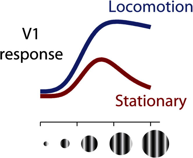
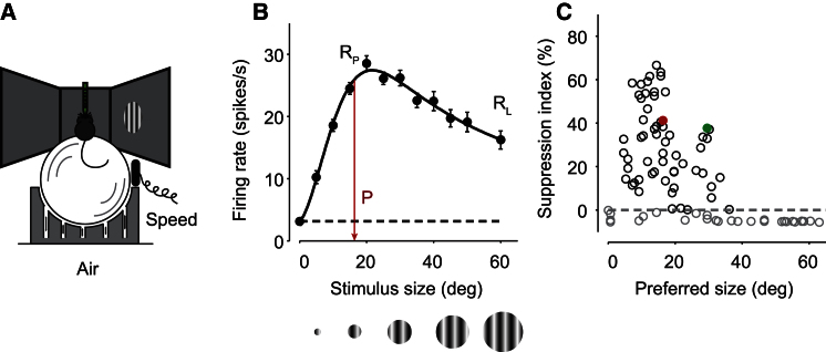
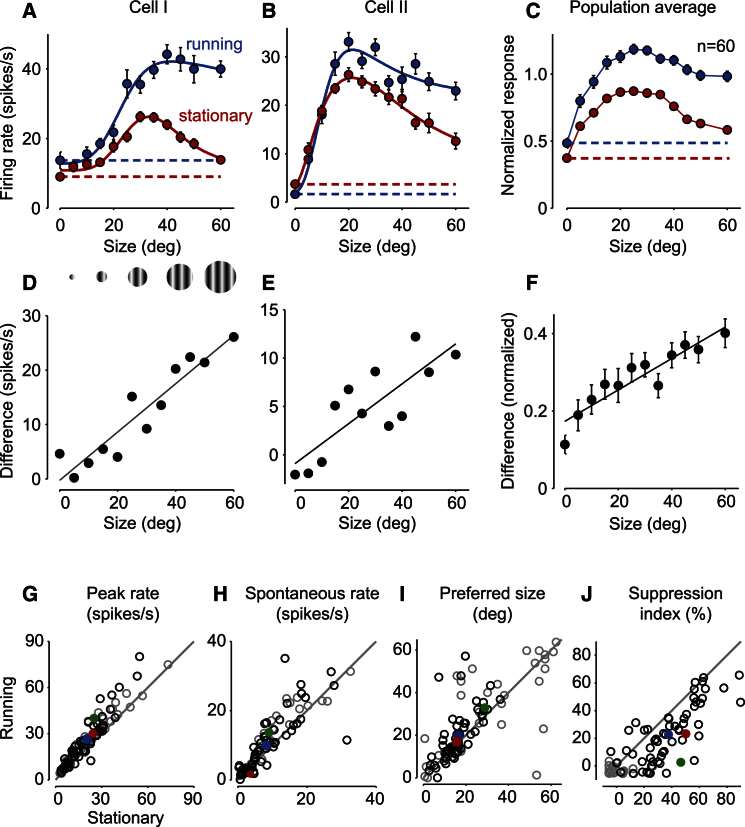
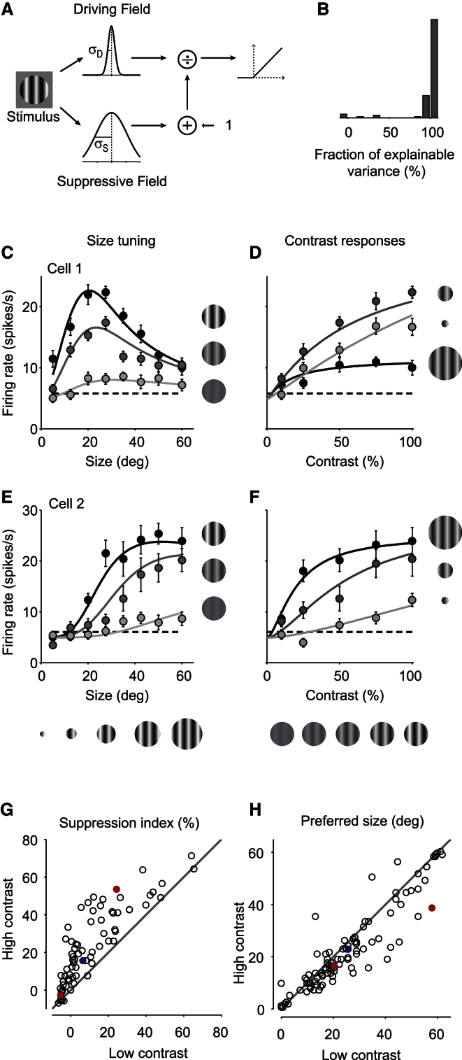
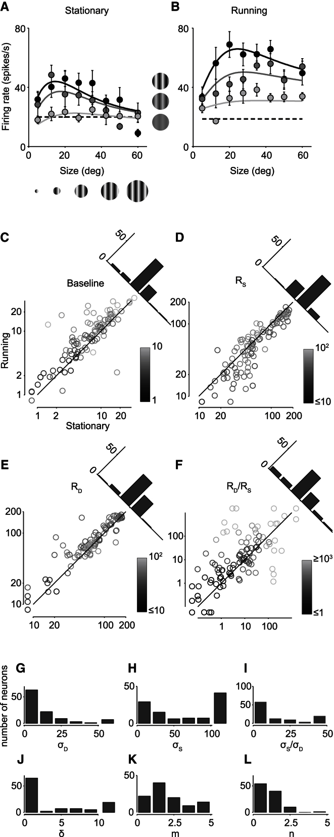
Growing evidence indicates that responses in sensory cortex are modulated by factors beyond direct sensory stimulation. In primary visual cortex (V1), for instance, responses increase with locomotion. Here we show that this increase is accompanied by a profound change in spatial integration. We recorded from V1 neurons in head-fixed mice placed on a spherical treadmill. We characterized spatial integration and found that the responses of most neurons were suppressed by large stimuli. As in primates, this surround suppression increased with stimulus contrast. These effects were captured by a divisive normalization model, where the numerator originates from a central region driving the neuron and the denominator originates from a larger suppressive field. We then studied the effects of locomotion and found that it markedly reduced surround suppression, allowing V1 neurons to integrate over larger regions of visual space. Locomotion had two main effects: it increased spontaneous activity, and it weakened the suppressive signals mediating normalization, relative to the driving signals. We conclude that a fundamental aspect of visual processing, spatial integration, is controlled by an apparently unrelated factor, locomotion. This control might operate through the mechanisms that are in place to deliver surround suppression.
Overview
The claims and statistics of this paper haven’t been checked yet.
Run the check — free, no account needed. It reads the open-access text and checks the sources it cites.
Integrity signals
Registry
Cites
Statistics
Figures
Verification
Claims the paper makes
The claims and statistics of this paper haven’t been checked yet.
Run the check — free, no account needed. It reads the open-access text and checks the sources it cites.
Claims other papers make about this one
Each is checked against this paper’s own text: does it say what the citing paper says it does?
In the citing paper
“However, the effects of locomotion on the spontaneous discharge rates of presumed pyramidal neurons recorded in other layers is more diverse”
From Waking state: rapid variations modulate neural and behavioral responses (2015) · cites this paper as Ayaz et al., 2013
Self-check
Percentages, sums and reported differences re-computed from the paper’s own numbers.
The self-check needs the paper’s full text.
Citations
Cites
Normalization as a canonical neural computation
Carandini, M., & Heeger, D. J. (2012) · Nature Reviews Neuroscience · doi:10.1038/nrn3136 · Cited by 1,906
Self-citationModulation of visual responses by behavioral state in mouse visual cortex
Niell, C. M., & Stryker, M. P. (2010) · Neuron · doi:10.1016/j.neuron.2010.01.033 · Cited by 1,483 · cited 7×
“In agreement with previous results [9], we found that locomotion increases both baseline activity and visually driven activity.”
BackgroundMethodResultInfluentialIs neocortex essentially multisensory?
GHAZANFAR, A., & SCHROEDER, C. (2006) · Trends in Cognitive Sciences · doi:10.1016/j.tics.2006.04.008 · Cited by 1,463
The Normalization Model of Attention
Reynolds, J. H., & Heeger, D. J. (2009) · Neuron · doi:10.1016/j.neuron.2009.01.002 · Cited by 1,457
Sparse Coding and Decorrelation in Primary Visual Cortex During Natural Vision
Vinje, W. E., & Gallant, J. L. (2000) · Science · doi:10.1126/science.287.5456.1273 · Cited by 1,286
Harris, K. D., & Thiele, A. (2011) · Nature reviews. Neuroscience · doi:10.1038/nrn3084 · Cited by 915
Natural signal statistics and sensory gain control
Schwartz, O., & Simoncelli, E. P. (2001) · Nature Neuroscience · doi:10.1038/90526 · Cited by 835
Nature and Interaction of Signals From the Receptive Field Center and Surround in Macaque V1 Neurons
Cavanaugh, J. R., Bair, W., & Movshon, J. A. (2002) · Journal of Neurophysiology · doi:10.1152/jn.00692.2001 · Cited by 784
A neural circuit for spatial summation in visual cortex
Adesnik, H., Bruns, W., Taniguchi, H., Huang, Z. J., & Scanziani, M. (2012) · Nature · doi:10.1038/nature11526 · Cited by 702
Sensorimotor mismatch signals in primary visual cortex of the behaving mouse
Keller, G. B., Bonhoeffer, T., & Hübener, M. (2012) · Neuron · doi:10.1016/j.neuron.2012.03.040 · Cited by 668
Cited by
Sorted by citations
Single-trial neural dynamics are dominated by richly varied movements
Musall, S., Kaufman, M. T., Juavinett, A., Gluf, S., & Churchland, A. K. (2019) · Nature Neuroscience · doi:10.1038/s41593-019-0502-4 · Cited by 1,102
A Cortical Circuit for Gain Control by Behavioral State
Fu, Y., Tucciarone, J. M., Espinosa, J. S., Sheng, N., Darcy, D. P., Nicoll, R. A., Huang, Z. J., & Stryker, M. P. (2014) · Cell · doi:10.1016/j.cell.2014.01.050 · Cited by 937
“Furthermore, besides increasing visual responses, locomotion has been shown to relieve surround suppression (Ayaz et al., 2013).”
BackgroundWaking state: rapid variations modulate neural and behavioral responses
McGinley, M. J., Vinck, M., Reimer, J., Batista-Brito, R., Zagha, E., Cadwell, C. R., Tolias, A. S., Cardin, J. A., & McCormick, D. A. (2015) · Neuron · doi:10.1016/j.neuron.2015.09.012 · Cited by 801
“However, the effects of locomotion on the spontaneous discharge rates of presumed pyramidal neurons recorded in other layers is more diverse (Ayaz et al., 2013; Beloozerova et al., 2003; Bennett et al., 2013; Nelson et al., 2013; Saleem et al., 2013; Schneider et al., 2014; Vinck et al., 2015; Zhou…”
Spike sorting for large, dense electrode arrays
Rossant, C., Kadir, S., Goodman, D. F. M., Schulman, J., Hunter, M. L. D., Saleem, A. B., Grosmark, A., Belluscio, M., Denfield, G. H., Ecker, A. S., et al. (2016) · Nature Neuroscience · doi:10.1038/nn.4268 · Cited by 800
Self-citationA Sensorimotor Circuit in Mouse Cortex for Visual Flow Predictions
Leinweber, M., Ward, D. R., Sobczak, J. M., Attinger, A., & Keller, G. B. (2017) · Neuron · doi:10.1016/j.neuron.2017.08.036 · Cited by 375
Diverse coupling of neurons to populations in sensory cortex
Okun, M., Steinmetz, N. A., Cossell, L., Iacaruso, M. F., Ko, H., Barthó, P., Moore, T., Hofer, S. B., Mrsic‐Flogel, T. D., Carandini, M., et al. (2015) · Nature · doi:10.1038/nature14273 · Cited by 429
Self-citationIntegration of visual motion and locomotion in mouse visual cortex
Saleem, A. B., Ayaz, A., Jeffery, K. J., Harris, K. D., & Carandini, M. (2013) · Nature Neuroscience · doi:10.1038/nn.3567 · Cited by 418
Self-citationSynaptic Scaling and Homeostatic Plasticity in the Mouse Visual Cortex In Vivo
Keck, T., Keller, G. B., Jacobsen, R. I., Eysel, U. T., Bonhoeffer, T., & Hübener, M. (2013) · Neuron · doi:10.1016/j.neuron.2013.08.018 · Cited by 367
Neuromodulation of brain state and behavior
McCormick, D. A., Nestvogel, D. B., & He, B. J. (2020) · Annual Review of Neuroscience · doi:10.1146/annurev-neuro-100219-105424 · Cited by 303
With or without you: predictive coding and Bayesian inference in the brain
Aitchison, L., & Lengyel, M. (2017) · Current Opinion in Neurobiology · doi:10.1016/j.conb.2017.08.010 · Cited by 308
Effects of locomotion extend throughout the mouse early visual system
Erisken, S., Vaiceliunaite, A., Jurjut, O., Fiorini, M., Katzner, S., & Busse, L. (2014) · Current Biology · doi:10.1016/j.cub.2014.10.045 · Cited by 256
Subthreshold mechanisms underlying state-dependent modulation of visual responses
Bennett, C., Arroyo, S., & Hestrin, S. (2013) · Neuron · doi:10.1016/j.neuron.2013.08.007 · Cited by 292
Vision and Locomotion Shape the Interactions between Neuron Types in Mouse Visual Cortex
Dipoppa, M., Ranson, A., Krumin, M., Pachitariu, M., Carandini, M., & Harris, K. D. (2018) · Neuron · doi:10.1016/j.neuron.2018.03.037 · Cited by 290
Self-citationIdentification of a brainstem circuit regulating visual cortical state in parallel with locomotion
Lee, A. M., Hoy, J. L., Bonci, A., Wilbrecht, L., Stryker, M. P., & Niell, C. M. (2014) · Neuron · doi:10.1016/j.neuron.2014.06.031 · Cited by 282
Coherent encoding of subjective spatial position in visual cortex and hippocampus
Saleem, A. B., Diamanti, E. M., Fournier, J., Harris, K. D., & Carandini, M. (2018) · Nature · doi:10.1038/s41586-018-0516-1 · Cited by 253
Self-citationThe Nature of Shared Cortical Variability
Lin, I.-C., Okun, M., Carandini, M., & Harris, K. D. (2015) · Neuron · doi:10.1016/j.neuron.2015.06.035 · Cited by 232
Self-citationRepresentational drift in the mouse visual cortex
Deitch, D., Rubin, A., & Ziv, Y. (2021) · Current Biology · doi:10.1016/j.cub.2021.07.062 · Cited by 241
Locomotion Enhances Neural Encoding of Visual Stimuli in Mouse V1
Dadarlat, M. C., & Stryker, M. P. (2017) · The Journal of Neuroscience · doi:10.1523/jneurosci.2728-16.2017 · Cited by 205
Zhao, X., Liu, M., & Cang, J. (2014) · Neuron · doi:10.1016/j.neuron.2014.08.037 · Cited by 212
Mismatch Receptive Fields in Mouse Visual Cortex
Zmarz, P., & Keller, G. B. (2016) · Neuron · doi:10.1016/j.neuron.2016.09.057 · Cited by 178
Zagha, E., & McCormick, D. A. (2014) · Current Opinion in Neurobiology · doi:10.1016/j.conb.2014.09.010 · Cited by 191
Somatostatin-Expressing Inhibitory Interneurons in Cortical Circuits
Yavorska, I., & Wehr, M. (2016) · Frontiers in Neural Circuits · doi:10.3389/fncir.2016.00076 · Cited by 185
Natural behavior is the language of the brain
Miller, C. T., Gire, D. H., Hoke, K. L., Huk, A. C., Kelley, D. B., Leopold, D. A., Smear, M. C., Theunissen, F. E., Yartsev, M. M., & Niell, C. M. (2022) · Current Biology · doi:10.1016/j.cub.2022.03.031 · Cited by 179
Visual Functions of the Thalamus
Usrey, W. M., & Alitto, H. J. (2015) · Annual Review of Vision Science · doi:10.1146/annurev-vision-082114-035920 · Cited by 175
Layer-specific integration of locomotion and sensory information in mouse barrel cortex
Ayaz, A., Stäuble, A., Hamada, M., Wulf, M.-A., Saleem, A. B., & Helmchen, F. (2019) · Nature Communications · doi:10.1038/s41467-019-10564-8 · Cited by 155
Self-citationMovement-Related Signals in Sensory Areas: Roles in Natural Behavior
Parker, P. R. L., Brown, M. A., Smear, M. C., & Niell, C. M. (2020) · Trends in Neurosciences · doi:10.1016/j.tins.2020.05.005 · Cited by 154
Subcortical Source and Modulation of the Narrowband Gamma Oscillation in Mouse Visual Cortex
Saleem, A. B., Lien, A. D., Krumin, M., Haider, B., Rosón, M. R., Ayaz, A., Reinhold, K., Busse, L., Carandini, M., & Harris, K. D. (2017) · Neuron · doi:10.1016/j.neuron.2016.12.028 · Cited by 154
Self-citationMineault, P. J., Tring, E., Trachtenberg, J. T., & Ringach, D. L. (2016) · The Journal of Neuroscience · doi:10.1523/jneurosci.0430-16.2016 · Cited by 148
Perception as a closed-loop convergence process
Ahissar, E., & Assa, E. (2016) · eLife · doi:10.7554/elife.12830 · Cited by 164
Inhibitory stabilization and visual coding in cortical circuits with multiple interneuron subtypes
Litwin-Kumar, A., Rosenbaum, R., & Doiron, B. (2016) · Journal of Neurophysiology · doi:10.1152/jn.00732.2015 · Cited by 146
Imaging the awake visual cortex with a genetically encoded voltage indicator
Carandini, M., Shimaoka, D., Rossi, L. F., Sato, T. K., Benucci, A., & Knöpfel, T. (2015) · The Journal of Neuroscience · doi:10.1523/jneurosci.0594-14.2015 · Cited by 115
Self-citationSynaptic Mechanisms of Feature Coding in the Visual Cortex of Awake Mice
Adesnik, H. (2017) · Neuron · doi:10.1016/j.neuron.2017.08.014 · Cited by 134
Canonical computations of cerebral cortex
Miller, K. D. (2016) · Current Opinion in Neurobiology · doi:10.1016/j.conb.2016.01.008 · Cited by 136
Subnetwork-Specific Homeostatic Plasticity in Mouse Visual Cortex In Vivo
Barnes, S. J., Sammons, R. P., Jacobsen, R. I., Mackie, J., Keller, G. B., & Keck, T. (2015) · Neuron · doi:10.1016/j.neuron.2015.05.010 · Cited by 123
Barnes, S. J., Franzoni, E., Jacobsen, R. I., Erdélyi, F., Szabó, G., Clopath, C., Keller, G. B., & Keck, T. (2017) · Neuron · doi:10.1016/j.neuron.2017.09.052 · Cited by 125
Walking enhances peripheral visual processing in humans
Cao, L., & Händel, B. (2019) · PLoS Biology · doi:10.1371/journal.pbio.3000511 · Cited by 121
Yoshida, T., & Ohki, K. (2020) · Nature Communications · doi:10.1038/s41467-020-14645-x · Cited by 122
The Cortical States of Wakefulness
Poulet, J. F. A., & Crochet, S. (2019) · Frontiers in Systems Neuroscience · doi:10.3389/fnsys.2018.00064 · Cited by 126
Fast Hemodynamic Responses in the Visual Cortex of the Awake Mouse
Pisauro, M. A., Dhruv, N. T., Carandini, M., & Benucci, A. (2013) · Journal of Neuroscience · doi:10.1523/jneurosci.2130-13.2013 · Cited by 115
Self-citationQuestioning the role of sparse coding in the brain
Spanne, A., & Jörntell, H. (2015) · Trends in Neurosciences · doi:10.1016/j.tins.2015.05.005 · Cited by 125
Layer-Specific Refinement of Visual Cortex Function after Eye Opening in the Awake Mouse
Hoy, J. L., & Niell, C. M. (2015) · Journal of Neuroscience · doi:10.1523/jneurosci.3174-14.2015 · Cited by 117
How Cortical Circuits Implement Cortical Computations: Mouse Visual Cortex as a Model
Niell, C. M., & Scanziani, M. (2021) · Annual Review of Neuroscience · doi:10.1146/annurev-neuro-102320-085825 · Cited by 120
Orientation-Tuned Surround Suppression in Mouse Visual Cortex
Self, M. W., Lorteije, J. A. M., Vangeneugden, J., van Beest, E. H., Grigore, M., Levelt, C. N., Heimel, J. A., & Roelfsema, P. R. (2014) · Journal of Neuroscience · doi:10.1523/jneurosci.5051-13.2014 · Cited by 109
Neural correlates of sparse coding and dimensionality reduction
Beyeler, M., Rounds, E. L., Carlson, K. D., Dutt, N., & Krichmar, J. L. (2019) · PLOS Computational Biology · doi:10.1371/journal.pcbi.1006908 · Cited by 104
Effects of Arousal on Mouse Sensory Cortex Depend on Modality
Shimaoka, D., Harris, K. D., & Carandini, M. (2018) · Cell Reports · doi:10.1016/j.celrep.2018.02.092 · Cited by 110
Self-citationLocomotor activity modulates associative learning in mouse cerebellum
Albergaria, C., Silva, N. T., Pritchett, D. L., & Carey, M. R. (2018) · Nature Neuroscience · doi:10.1038/s41593-018-0129-x · Cited by 97
Kafashan, M., Jaffe, A. W., Chettih, S. N., Nogueira, R., Arandia-Romero, I., Harvey, C. D., Moreno-Bote, R., & Drugowitsch, J. (2021) · Nature Communications · doi:10.1038/s41467-020-20722-y · Cited by 96
Cortico-cortical feedback engages active dendrites in visual cortex
Fişek, M., Herrmann, D., Egea-Weiss, A., Cloves, M., Bauer, L., Lee, T.-Y., Russell, L. E., & Häusser, M. (2023) · Nature · doi:10.1038/s41586-023-06007-6 · Cited by 80
FISSA: A neuropil decontamination toolbox for calcium imaging signals
Keemink, S. W., Lowe, S., Pakan, J. M. P., Dylda, E., van Rossum, M. C. W., & Rochefort, N. L. (2018) · Scientific Reports · doi:10.1038/s41598-018-21640-2 · Cited by 87
Michaiel, A. M., Parker, P. R. L., & Niell, C. M. (2019) · Cell Reports · doi:10.1016/j.celrep.2019.02.104 · Cited by 82
Diversity and Function of Somatostatin-Expressing Interneurons in the Cerebral Cortex
Riedemann, T. (2019) · International Journal of Molecular Sciences · doi:10.3390/ijms20122952 · Cited by 103
Spatial integration in mouse primary visual cortex
Vaičeliūnaitė, A., Erisken, S., Franzen, F., Katzner, S., & Busse, L. (2013) · Journal of Neurophysiology · doi:10.1152/jn.00138.2013 · Cited by 85
Invariant visual object recognition and shape processing in rats
Zoccolan, D. (2015) · Behavioural Brain Research · doi:10.1016/j.bbr.2014.12.053 · Cited by 91
Virtual reality systems for rodents
Thurley, K., & Ayaz, A. (2016) · Current Zoology · doi:10.1093/cz/zow070 · Cited by 90
Self-citationContextual signals in visual cortex
Khan, A. G., & Hofer, S. B. (2018) · Current Opinion in Neurobiology · doi:10.1016/j.conb.2018.05.003 · Cited by 83
Sensation during Active Behaviors
Busse, L., Cardin, J. A., Chiappe, M. E., Halassa, M. M., McGinley, M. J., Yamashita, T., & Saleem, A. B. (2017) · Journal of Neuroscience · doi:10.1523/jneurosci.1828-17.2017 · Cited by 84
Self-citationLocomotion modulates specific functional cell types in the mouse visual thalamus
Aydın, Ç., Couto, J., Giugliano, M., Farrow, K., & Bonin, V. (2018) · Nature Communications · doi:10.1038/s41467-018-06780-3 · Cited by 73
Visually Cued Action Timing in the Primary Visual Cortex
Namboodiri, V. M. K., Huertas, M. A., Monk, K. J., Shouval, H. Z., & Shuler, M. G. H. (2015) · Neuron · doi:10.1016/j.neuron.2015.02.043 · Cited by 79
Functional modulation of primary visual cortex by the superior colliculus in the mouse
Ahmadlou, M., Zweifel, L. S., & Heimel, J. A. (2018) · Nature Communications · doi:10.1038/s41467-018-06389-6 · Cited by 81
Action and learning shape the activity of neuronal circuits in the visual cortex
Pakan, J. M. P., Francioni, V., & Rochefort, N. L. (2018) · Current Opinion in Neurobiology · doi:10.1016/j.conb.2018.04.020 · Cited by 75
Encoding sensory and motor patterns as time-invariant trajectories in recurrent neural networks
Goudar, V., & Buonomano, D. V. (2018) · eLife · doi:10.7554/elife.31134 · Cited by 77
Cell Types, Circuits, and Receptive Fields in the Mouse Visual Cortex
Niell, C. M. (2015) · Annual Review of Neuroscience · doi:10.1146/annurev-neuro-071714-033807 · Cited by 78
Encoding of 3D Head Orienting Movements in the Primary Visual Cortex
Guitchounts, G., Masis, J. A., Wolff, S. B. E., & Cox, D. (2020) · Neuron · doi:10.1016/j.neuron.2020.07.014 · Cited by 72
Not so spontaneous: Multi-dimensional representations of behaviors and context in sensory areas
Avitan, L., & Stringer, C. (2022) · Neuron · doi:10.1016/j.neuron.2022.06.019 · Cited by 71
Joint coding of visual input and eye/head position in V1 of freely moving mice
Parker, P. R. L., Abe, E. T. T., Leonard, E. S. P., Martins, D. M., & Niell, C. M. (2022) · Neuron · doi:10.1016/j.neuron.2022.08.029 · Cited by 78
Activity in primate visual cortex is minimally driven by spontaneous movements
Talluri, B. C., Kang, I., Lazere, A., Quinn, K. R., Kaliss, N., Yates, J. L., Butts, D. A., & Nienborg, H. (2023) · Nature Neuroscience · doi:10.1038/s41593-023-01459-5 · Cited by 83
Precise movement-based predictions in the mouse auditory cortex
Audette, N. J., Zhou, W., Chioma, A. L., & Schneider, D. M. (2022) · Current Biology · doi:10.1016/j.cub.2022.09.064 · Cited by 95
Movement and VIP Interneuron Activation Differentially Modulate Encoding in Mouse Auditory Cortex
Bigelow, J., Morrill, R. J., DeKloe, J., & Hasenstaub, A. R. (2019) · eNeuro · doi:10.1523/eneuro.0164-19.2019 · Cited by 66
Three brain states in the hippocampus and cortex
Kay, K., & Frank, L. M. (2018) · Hippocampus · doi:10.1002/hipo.22956 · Cited by 69
Stable Encoding of Visual Cues in the Mouse Retrosplenial Cortex
Powell, A. L., Connelly, W. M., Vasalauskaite, A., Nelson, A. J. D., Vann, S. D., Aggleton, J. P., Sengpiel, F., & Ranson, A. (2020) · Cerebral Cortex · doi:10.1093/cercor/bhaa030 · Cited by 65
Audio-visual experience strengthens multisensory assemblies in adult mouse visual cortex
Knöpfel, T., Sweeney, Y., Radulescu, C. I., Zabouri, N., Doostdar, N., Clopath, C., & Barnes, S. J. (2019) · Nature Communications · doi:10.1038/s41467-019-13607-2 · Cited by 68
Tasks and their role in visual neuroscience
Kay, K., Bonnen, K., Denison, R. N., Arcaro, M. J., & Barack, D. L. (2023) · Neuron · doi:10.1016/j.neuron.2023.03.022 · Cited by 61
Feature-Specific Organization of Feedback Pathways in Mouse Visual Cortex
Huh, C. Y. L., Peach, J. P., Bennett, C., Vega, R. M., & Hestrin, S. (2017) · Current Biology · doi:10.1016/j.cub.2017.11.056 · Cited by 62
Garrett, J., Chak, C., Bullock, T., & Giesbrecht, B. (2024) · Communications Psychology · doi:10.1038/s44271-024-00124-2 · Cited by 76
Acute Exercise Modulates Feature-selective Responses in Human Cortex
Bullock, T., Elliott, J. C., Serences, J. T., & Giesbrecht, B. (2016) · Journal of Cognitive Neuroscience · doi:10.1162/jocn_a_01082 · Cited by 56
Chen, J. L., Andermann, M. L., Keck, T., Xu, N.-L., & Ziv, Y. (2013) · Journal of Neuroscience · doi:10.1523/jneurosci.3255-13.2013 · Cited by 58
Lakunina, A. A., Nardoci, M. B., Ahmadian, Y., & Jaramillo, S. (2020) · Journal of Neuroscience · doi:10.1523/jneurosci.1735-19.2020 · Cited by 55
Effects of Locomotion on Visual Responses in the Mouse Superior Colliculus
Savier, E. L., Chen, H., & Cang, J. (2019) · Journal of Neuroscience · doi:10.1523/jneurosci.1854-19.2019 · Cited by 54
Multiple stages of information processing are modulated during acute bouts of exercise
Bullock, T., Cecotti, H., & Giesbrecht, B. (2015) · Neuroscience · doi:10.1016/j.neuroscience.2015.08.046 · Cited by 55
Behavior-dependent directional tuning in the human visual-navigation network
Nau, M., Schröder, T. N., Frey, M., & Doeller, C. F. (2020) · Nature Communications · doi:10.1038/s41467-020-17000-2 · Cited by 53
Arousal regulates frequency tuning in primary auditory cortex
Lin, P.-A., Asinof, S. K., Edwards, N. J., & Isaacson, J. S. (2019) · Proceedings of the National Academy of Sciences · doi:10.1073/pnas.1911383116 · Cited by 51
Behavioral decomposition reveals rich encoding structure employed across neocortex in rats
Mimica, B., Tombaz, T., Battistin, C., Fuglstad, J. G., Dunn, B. A., & Whitlock, J. R. (2023) · Nature Communications · doi:10.1038/s41467-023-39520-3 · Cited by 45
The Effect of Locomotion on Early Visual Contrast Processing in Humans
Benjamin, A. V., Wailes-Newson, K. H., Ma-Wyatt, A., Baker, D. H., & Wade, A. R. (2018) · Journal of Neuroscience · doi:10.1523/jneurosci.1428-17.2017 · Cited by 47
Improved deep two-photon calcium imaging in vivo
Birkner, A., Tischbirek, C. H., & Konnerth, A. (2016) · Cell Calcium · doi:10.1016/j.ceca.2016.12.005 · Cited by 46
Reduced neural activity but improved coding in rodent higher-order visual cortex during locomotion
Christensen, A. J., & Pillow, J. W. (2022) · Nature Communications · doi:10.1038/s41467-022-29200-z · Cited by 46
Cortical sensory processing across motivational states during goal-directed behavior
Matteucci, G., Guyoton, M., Mayrhofer, J. M., Auffret, M., Foustoukos, G., Petersen, C. C. H., & El‐Boustani, S. (2022) · Neuron · doi:10.1016/j.neuron.2022.09.032 · Cited by 43
Thalamus Controls Development and Expression of Arousal States in Visual Cortex
Murata, Y., & Colonnese, M. T. (2018) · Journal of Neuroscience · doi:10.1523/jneurosci.1519-18.2018 · Cited by 44
Overground Walking Decreases Alpha Activity and Entrains Eye Movements in Humans
Cao, L., Chen, X., & Händel, B. (2020) · Frontiers in Human Neuroscience · doi:10.3389/fnhum.2020.561755 · Cited by 42
Temporal stability of stimulus representation increases along rodent visual cortical hierarchies
Piasini, E., Soltuzu, L., Muratore, P., Caramellino, R., Vinken, K., de Beeck, H. O., Balasubramanian, V., & Zoccolan, D. (2021) · Nature Communications · doi:10.1038/s41467-021-24456-3 · Cited by 44
Higher brain functions served by the lowly rodent primary visual cortexPreprint
Gavornik, J. P., & Bear, M. F. (2014) · Learning & Memory · doi:10.1101/lm.034355.114 · Cited by 42
Tang, M. F., Kheradpezhouh, E., Lee, C. C. Y., Dickinson, J. E., Mattingley, J. B., & Arabzadeh, E. (2023) · Nature Communications · doi:10.1038/s41467-023-36608-8 · Cited by 47
Top-Down Suppression of Sensory Cortex in an NMDAR Hypofunction Model of Psychosis
Ranson, A., Broom, E., Powell, A. L., Chen, F., Major, G., & Hall, J. (2019) · Schizophrenia Bulletin · doi:10.1093/schbul/sby190 · Cited by 40
Perceptual Decision-Making: A Field in the Midst of a Transformation
Najafi, F., & Churchland, A. K. (2018) · Neuron · doi:10.1016/j.neuron.2018.10.017 · Cited by 41
Rapid and active stabilization of visual cortical firing rates across light–dark transitions
Pacheco, A. T., Tilden, E. I., Grutzner, S. M., Lane, B. J., Wu, Y. K., Hengen, K. B., Gjorgjieva, J., & Turrigiano, G. G. (2019) · Proceedings of the National Academy of Sciences · doi:10.1073/pnas.1906595116 · Cited by 37
Magnetic tracking of eye position in freely behaving chickens
Schwarz, J. S., Sridharan, D., & Knudsen, E. I. (2013) · Frontiers in Systems Neuroscience · doi:10.3389/fnsys.2013.00091 · Cited by 38
Sensory experience steers representational drift in mouse visual cortex
Bauer, J., Lewin, U., Herbert, E., Gjorgjieva, J., Schoonover, C. E., Fink, A. J. P., Rose, T., Bonhoeffer, T., & Hübener, M. (2024) · Nature Communications · doi:10.1038/s41467-024-53326-x · Cited by 42
Temporal Processing in the Visual Cortex of the Awake and Anesthetized Rat
Aasebø, I. E. J., Lepperød, M. E., Stavrinou, M., Nøkkevangen, S., Einevoll, G. T., Hafting, T., & Fyhn, M. (2017) · eNeuro · doi:10.1523/eneuro.0059-17.2017 · Cited by 38
Wagatsuma, N., Nobukawa, S., & Fukai, T. (2022) · Cerebral Cortex · doi:10.1093/cercor/bhac355 · Cited by 35
Differential effects of walking across visual cortical processing stages
Chen, X., Cao, L., & Händel, B. (2022) · Cortex · doi:10.1016/j.cortex.2022.01.007 · Cited by 34
Visual Cortex Limits Pop-Out in the Superior Colliculus of Awake Mice
Ahmadlou, M., Tafreshiha, A., & Heimel, J. A. (2017) · Cerebral Cortex · doi:10.1093/cercor/bhx254 · Cited by 35
Metadata
- Authors
- Ayaz, A., Saleem, A. B., Schölvinck, M. L., & Carandini, M.
- Affiliations
- University College London (GB)
- Corresponding author
- Ayaz, Aslı
- Venue
- Current Biology
- Publisher
- Elsevier BV
- Published
- 2013-05
- Volume
- 23
- Issue
- 10
- Pages
- 890-894
- ISSN
- 0960-9822 (ISSN-L)
- PMC
- PMC3661981
- OpenAlex
- W2057290285
- Cited by
- 249
- References
- 27
- Citations by year
- 2026: 8 · 2025: 17 · 2024: 28 · 2023: 21 · 2022: 22 · 2021: 17 · 2020: 19 · 2019: 21 · 2018: 28 · 2017: 20 · 2016: 14 · 2015: 16 · 2014: 10 · 2013: 8
- FWCI
- 8.78
- Type
- journal article
- Language
- en
- Open access
- hybrid
- doi.org
- Licence
- Locations
- Current Biology (publishedVersion, cc-by)
- Europe PMC (PubMed Central) (publishedVersion, cc-by)
- PubMed Central (publishedVersion, cc-by)
- PubMed (publishedVersion)
- UCL Discovery (University College London) (submittedVersion)
- Funders
- European Research Council
- Wellcome Trust
- Medical Research Council
- Topics
- Life Sciences › Neuroscience › Cognitive Neuroscience › Visual perception and processing mechanisms
- Social Sciences › Psychology › Experimental and Cognitive Psychology › Multisensory perception and integration
- Life Sciences › Neuroscience › Cellular and Molecular Neuroscience › Neuroscience and Neuropharmacology Research
- Keywords
- locomotion, primary visual cortex, spatial integration, surround suppression, divisive normalization, spontaneous activity, stimulus contrast, mouse visual cortex
- MeSH terms
- Animals, Locomotion, Space Perception, Visual Cortex, Mice
About these checks
Registry, retraction, Cites and statistics results are computed, not judged, with one exception: a printed reference that no index lists is read once by a model before it counts as a citation error. Claims are extracted by a model and kept only when their quote appears verbatim in the text; each cited source is then checked, with a model’s help, for whether it says what the claim relies on. Those verdicts can be wrong — read the claim’s quote and the cited source before relying on one.
Statistics and arithmetic are recomputed, not judged.
Confidence bands are shown only for fields calibrated on our annotated test set. None is calibrated yet, so no band is shown.
What counts as a claim ›How we measure confidence ›How we check this ›
Are you an author, or do you see a problem with this page? Request a review
