Cited by 69Genetic Associations and EpidemiologyBioinformatics and Genomic NetworksGenetic Mapping and Diversity in Plants and Animals

The DOI matches its Crossref record; 50 of the 50 references it cites were found in a registry or an index.

Exploring the phenotypic consequences of tissue specific gene expression variation inferred from GWAS summary statistics

Open access
Barbeira, Alvaro N., Dickinson, Scott P., Bonazzola, Rodrigo, Zheng, Jiamao, Wheeler, Heather E., Torres, Jason M., Torstenson, Eric S., Shah, Kaanan P., Garcia, Tzintzuni, Edwards, Todd L., Stahl, Eli A., Huckins, Laura M., GTEx Consortium, Laboratory, Data Analysis & Coordinating Center (LDACC)—Analysis Working Group, Aguet, François, Ardlie, Kristin G., Cummings, Beryl B., Gelfand, Ellen T., Getz, Gad, Hadley, Kane, Handsaker, Robert E., Huang, Katherine H., Kashin, Seva, Karczewski, Konrad J., Lek, Monkol, Li, Xiao, MacArthur, Daniel G., Nedzel, Jared L., Nguyen, Duyen T., Noble, Michael S., Segrè, Ayellet V., Trowbridge, Casandra A., Tukiainen, Taru, Statistical Methods groups—Analysis Working Group, Abell, Nathan S., Balliu, Brunilda, Barshir, Ruth, Basha, Omer, Battle, Alexis, Bogu, Gireesh K., Brown, Andrew, Brown, Christopher D., Castel, Stephane E., Chen, Lin S., Chiang, Colby, Conrad, Donald F., Damani, Farhan N., Davis, Joe R., Delaneau, Olivier, Dermitzakis, Emmanouil T., Engelhardt, Barbara E., Eskin, Eleazar, Ferreira, Pedro G., Frésard, Laure, Gamazon, Eric R., Garrido-Martín, Diego, Gewirtz, Ariel D. H., Gliner, Genna, Gloudemans, Michael J., Guigo, Roderic, Hall, Ira M., Han, Buhm, He, Yuan, Hormozdiari, Farhad, Howald, Cedric, Jo, Brian, Kang, Eun Yong, Kim, Yungil, Kim-Hellmuth, Sarah, Lappalainen, Tuuli, Li, Gen, Li, Xin, Liu, Boxiang, Mangul, Serghei, McCarthy, Mark I., McDowell, Ian C., Mohammadi, Pejman, Monlong, Jean, Montgomery, Stephen B., Muñoz-Aguirre, Manuel, Ndungu, Anne W., Nobel, Andrew B., Oliva, Meritxell, Ongen, Halit, Palowitch, John J., Panousis, Nikolaos, Papasaikas, Panagiotis, Park, YoSon, Parsana, Princy, Payne, Anthony J., Peterson, Christine B., Quan, Jie, Reverter, Ferran, Sabatti, Chiara, Saha, Ashis, Sammeth, Michael, Scott, Alexandra J., Shabalin, Andrey A., Sodaei, Reza, Stephens, Matthew, Stranger, Barbara E., Strober, Benjamin J., Sul, Jae Hoon, Tsang, Emily K., Urbut, Sarah, van de Bunt, Martijn, Wang, Gao, Wen, Xiaoquan, Wright, Fred A., Xi, Hualin S., Yeger-Lotem, Esti, Zappala, Zachary, Zaugg, Judith B., Zhou, Yi-Hui, Enhancing GTEx (eGTEx) groups, Akey, Joshua M., Bates, Daniel, Chan, Joanne, Chen, Lin S., Claussnitzer, Melina, Demanelis, Kathryn, Diegel, Morgan, Doherty, Jennifer A., Feinberg, Andrew P., Fernando, Marian S., Halow, Jessica, Hansen, Kasper D., Haugen, Eric, Hickey, Peter F., Hou, Lei, Jasmine, Farzana, Jian, Ruiqi, Jiang, Lihua, Johnson, Audra, Kaul, Rajinder, Kellis, Manolis, Kibriya, Muhammad G., Lee, Kristen, Li, Jin Billy, Li, Qin, Li, Xiao, Lin, Jessica, Lin, Shin, Linder, Sandra, Linke, Caroline, Liu, Yaping, Maurano, Matthew T., Molinie, Benoit, Montgomery, Stephen B., Nelson, Jemma, Neri, Fidencio J., Oliva, Meritxell, Park, Yongjin, Pierce, Brandon L., Rinaldi, Nicola J., Rizzardi, Lindsay F., Sandstrom, Richard, Skol, Andrew, Smith, Kevin S., Snyder, Michael P., Stamatoyannopoulos, John, Stranger, Barbara E., Tang, Hua, Tsang, Emily K., Wang, Li, Wang, Meng, Van Wittenberghe, Nicholas, Wu, Fan, Zhang, Rui, NIH Common Fund, Nierras, Concepcion R., NIH/NCI, Branton, Philip A., Carithers, Latarsha J., Guan, Ping, Moore, Helen M., Rao, Abhi, Vaught, Jimmie B., NIH/NHGrI, Gould, Sarah E., Lockart, Nicole C., Martin, Casey, Struewing, Jeffery P., Volpi, Simona, NIH/NIMH, Addington, Anjene M., Koester, Susan E., NIH/NIDA, Little, A. Roger, Biospecimen Collection Source Site—NDrI, Brigham, Lori E., Hasz, Richard, Hunter, Marcus, Johns, Christopher, Johnson, Mark, Kopen, Gene, Leinweber, William F., Lonsdale, John T., McDonald, Alisa, Mestichelli, Bernadette, Myer, Kevin, Roe, Brian, Salvatore, Michael, Shad, Saboor, Thomas, Jeffrey A., Walters, Gary, Washington, Michael, Wheeler, Joseph, Biospecimen Collection Source Site—rPCI, Bridge, Jason, Foster, Barbara A., Gillard, Bryan M., Karasik, Ellen, Kumar, Rachna, Miklos, Mark, Moser, Michael T., Biospecimen Core resource—VArI, Jewell, Scott D., Montroy, Robert G., Rohrer, Daniel C., Valley, Dana R., Brain Bank repository—University of Miami Brain Endowment Bank, Davis, David A., Mash, Deborah C., Leidos Biomedical—Project Management, Undale, Anita H., Smith, Anna M., Tabor, David E., Roche, Nancy V., McLean, Jeffrey A., Vatanian, Negin, Robinson, Karna L., Sobin, Leslie, Barcus, Mary E., Valentino, Kimberly M., Qi, Liqun, Hunter, Steven, Hariharan, Pushpa, Singh, Shilpi, Um, Ki Sung, Matose, Takunda, Tomaszewski, Maria M., ELSI Study, Barker, Laura K., Mosavel, Maghboeba, Siminoff, Laura A., Traino, Heather M., Genome Browser Data Integration & Visualization—EBI, Flicek, Paul, Juettemann, Thomas, Ruffier, Magali, Sheppard, Dan, Taylor, Kieron, Trevanion, Stephen J., Zerbino, Daniel R., Genome Browser Data Integration & Visualization—UCSC Genomics Institute, University of California Santa Cruz, Craft, Brian, Goldman, Mary, Haeussler, Maximilian, Kent, W. James, Lee, Christopher M., Paten, Benedict, Rosenbloom, Kate R., Vivian, John, Zhu, Jingchun, Nicolae, Dan L., Cox, Nancy J., Im, Hae Kyung·2018·Nature Communications

Published version of a preprint

Abstract

Scalable, integrative methods to understand mechanisms that link genetic variants with phenotypes are needed. Here we derive a mathematical expression to compute PrediXcan (a gene mapping approach) results using summary data (S-PrediXcan) and show its accuracy and general robustness to misspecified reference sets. We apply this framework to 44 GTEx tissues and 100+ phenotypes from GWAS and meta-analysis studies, creating a growing public catalog of associations that seeks to capture the effects of gene expression variation on human phenotypes. Replication in an independent cohort is shown. Most of the associations are tissue specific, suggesting context specificity of the trait etiology. Colocalized significant associations in unexpected tissues underscore the need for an agnostic scanning of multiple contexts to improve our ability to detect causal regulatory mechanisms. Monogenic disease genes are enriched among significant associations for related traits, suggesting that smaller alterations of these genes may cause a spectrum of milder phenotypes.

Overview

The claims and statistics of this paper haven’t been checked yet.

Run the check — free, no account needed. It reads the open-access text and checks the sources it cites.

A few free checks a day · papers already verified open instantly · results are public

Integrity signals

Registry

Crossref · 10.1038/s41467-018-03621-1

Cites

50 of 50 references verified0 citation errors · 0 not checkable

Statistics

Figures

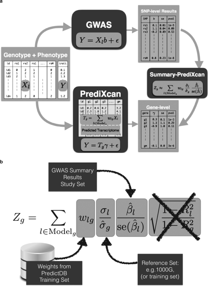
Fig. 1 Comparison between GWAS, PrediXcan, and S-PrediXcan. a Compares GWAS, PrediXcan, and Summary-PrediXcan. Both GWAS and PrediXcan take genotype and phenotype data as input. GWAS computes the regression coefficients of Y on Xl using the model Y=a+Xlb+ϵ, where Y is the phenotype and Xl the individual SNP dosage. The output is a table of SNP-level results. PrediXcan, in contrast, starts first by predicting/imputing the transcriptome. Then it calculates the regression coefficients of the phenotype Y on each gene’s predicted expression Tg. The output is a table of gene-level results. Summary-PrediXcan directly computes the gene-level association results using the output from GWAS. b Shows the components of the formula to calculate PrediXcan gene-level association results using summary statistics. The different sets involved as input data are shown. The regression coefficient between the phenotype and the genotype is obtained from the study set. The training set is the reference transcriptome dataset where the prediction models of gene expression levels are trained. The reference set (1000G, or training set having some advantages) is used to compute the variances and covariances (LD structure) of the markers used in the predicted expression levels. Both the reference set and training set values are precomputed and provided to the user so that only the study set results need to be provided to the software. The crossed out term was set to 1 as an approximation. We found this approximation to have negligible impact on the results
Fig. 1 Comparison between GWAS, PrediXcan, and S-PrediXcan. a Compares GWAS, PrediXcan, and Summary-PrediXcan. Both GWAS and PrediXcan take genotype and phenotype data as input. GWAS computes the regression coefficients of Y on Xl using the model Y=a+Xlb+ϵ, where Y is the phenotype and Xl the individual SNP dosage. The output is a table of SNP-level results. PrediXcan, in contrast, starts first by predicting/imputing the transcriptome. Then it calculates the regression coefficients of the phenotype Y on each gene’s predicted expression Tg. The output is a table of gene-level results. Summary-PrediXcan directly computes the gene-level association results using the output from GWAS. b Shows the components of the formula to calculate PrediXcan gene-level association results using summary statistics. The different sets involved as input data are shown. The regression coefficient between the phenotype and the genotype is obtained from the study set. The training set is the reference transcriptome dataset where the prediction models of gene expression levels are trained. The reference set (1000G, or training set having some advantages) is used to compute the variances and covariances (LD structure) of the markers used in the predicted expression levels. Both the reference set and training set values are precomputed and provided to the user so that only the study set results need to be provided to the software. The crossed out term was set to 1 as an approximation. We found this approximation to have negligible impact on the resultsCC BY · PubMed Central
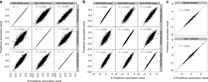
Fig. 2 Comparison of PrediXcan and S-PrediXcan results in real and simulated traits. This figure shows a comparison of PrediXcan vs. S-PrediXcan for a a simulated phenotype under null hypothesis of no genetic component; b a cellular phenotype (=intrinsic growth); and c bipolar disorder and type 1 diabetes studies from Wellcome Trust Case Control Consortium (WTCCC). Gene expression prediction models were based on the DGN cohort presented in ref. 11. For the simulated phenotype, study sets (GWAS set) and reference sets (LD calculation set) consisted of African (661), East Asian (504), and European (503) individuals from the 1000 Genomes Project. When the same study set is used as reference set, we obtained a high correlation (coefficient of determination): r2 > 0.99999. For the intrinsic growth phenotype, study sets were a subset of 140 individuals from each of the African, Asian, and European groups from 1000 Genomes Project. The reference set was the same as for the simulated phenotype. For the disease phenotypes, the study set consisted of British individuals, and the LD calculation set was the European population subset of the 1000 Genomes Project
Fig. 2 Comparison of PrediXcan and S-PrediXcan results in real and simulated traits. This figure shows a comparison of PrediXcan vs. S-PrediXcan for a a simulated phenotype under null hypothesis of no genetic component; b a cellular phenotype (=intrinsic growth); and c bipolar disorder and type 1 diabetes studies from Wellcome Trust Case Control Consortium (WTCCC). Gene expression prediction models were based on the DGN cohort presented in ref. 11. For the simulated phenotype, study sets (GWAS set) and reference sets (LD calculation set) consisted of African (661), East Asian (504), and European (503) individuals from the 1000 Genomes Project. When the same study set is used as reference set, we obtained a high correlation (coefficient of determination): r2 > 0.99999. For the intrinsic growth phenotype, study sets were a subset of 140 individuals from each of the African, Asian, and European groups from 1000 Genomes Project. The reference set was the same as for the simulated phenotype. For the disease phenotypes, the study set consisted of British individuals, and the LD calculation set was the European population subset of the 1000 Genomes ProjectCC BY · PubMed Central
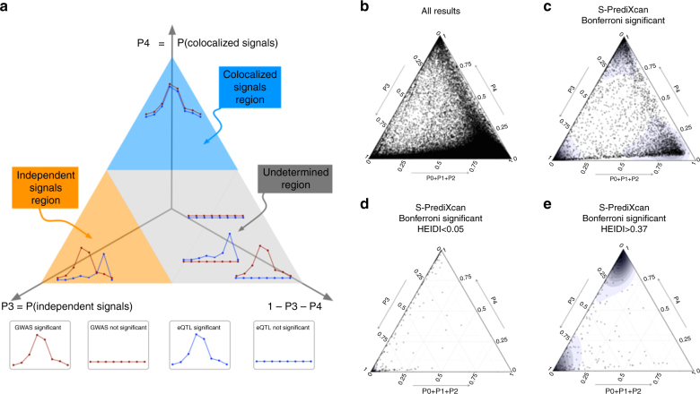
Fig. 3 Colocalization status of S-PrediXcan results. a Shows a ternary plot that represents the probabilities of various configurations from COLOC. This plot conveniently constrains the values such that the sum of the probabilities is 1. All points in a horizontal line have the same probability of “colocalized” GWAS and eQTL signals (P4), points on a line parallel to the right side of the triangle (NW to SE) have the same probability of “Independent signals” (P3), and lines parallel to the left side of the triangle (NE to SW) correspond to constant P0+P1+P2. Top sub-triangle in blue corresponds to high probability of colocalization (P4 > 0.5), lower left sub-triangle in orange corresponds to probability of independent signals (P3 > 0.5), and lower right parallelogram corresponds to genes without enough power to determine or reject colocalization. The following panels present ternary plots of COLOC probabilities with a density overlay for S-PrediXcan results of the Height phenotype. b Shows the colocalization probabilities for all gene-tissue pairs. Most results fall into the “undetermined” region. c Shows that if we keep only Bonferroni-significant S-PrediXcan results, associations tend to cluster into three distinct regions: “independent signals,” “colocalized,” and “undertermined.” d Shows that HEIDI significant genes (to be interpreted as high heterogeneity between GWAS and eQTL signals, i.e., distinct signals) tightly cluster in the “independent signal” region, in concordance with COLOC. A few genes fall in the “colocalized” region, in disagreement with COLOC classification. Unlike COLOC results, HEIDI does not partition the genes into distinct clusters and an arbitrary cutoff p-value has to be chosen. e Shows genes with large HEIDI p-value (no evidence of heterogeneity) which fall in large part in the “colocalized” region. However a substantial number fall in “independent signal” region, disagreeing with COLOC’s classification
Fig. 3 Colocalization status of S-PrediXcan results. a Shows a ternary plot that represents the probabilities of various configurations from COLOC. This plot conveniently constrains the values such that the sum of the probabilities is 1. All points in a horizontal line have the same probability of “colocalized” GWAS and eQTL signals (P4), points on a line parallel to the right side of the triangle (NW to SE) have the same probability of “Independent signals” (P3), and lines parallel to the left side of the triangle (NE to SW) correspond to constant P0+P1+P2. Top sub-triangle in blue corresponds to high probability of colocalization (P4 > 0.5), lower left sub-triangle in orange corresponds to probability of independent signals (P3 > 0.5), and lower right parallelogram corresponds to genes without enough power to determine or reject colocalization. The following panels present ternary plots of COLOC probabilities with a density overlay for S-PrediXcan results of the Height phenotype. b Shows the colocalization probabilities for all gene-tissue pairs. Most results fall into the “undetermined” region. c Shows that if we keep only Bonferroni-significant S-PrediXcan results, associations tend to cluster into three distinct regions: “independent signals,” “colocalized,” and “undertermined.” d Shows that HEIDI significant genes (to be interpreted as high heterogeneity between GWAS and eQTL signals, i.e., distinct signals) tightly cluster in the “independent signal” region, in concordance with COLOC. A few genes fall in the “colocalized” region, in disagreement with COLOC classification. Unlike COLOC results, HEIDI does not partition the genes into distinct clusters and an arbitrary cutoff p-value has to be chosen. e Shows genes with large HEIDI p-value (no evidence of heterogeneity) which fall in large part in the “colocalized” region. However a substantial number fall in “independent signal” region, disagreeing with COLOC’s classificationCC BY · PubMed Central
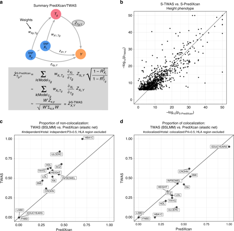
Fig. 4 Comparison between S-PrediXcan and S-TWAS. a Depicts how summary-TWAS and PrediXcan test the mediating role of gene expression level Tg. Multiple SNPs are linked to the expression level of a gene via weights wX,Tg. b Shows the significance of Summary-TWAS (BSLMM) vs. summary-PrediXcan (elastic net), for the height phenotype across 44 GTEx tissues. There is a small bias caused by using S-TWAS results available from24, which only lists significant hits. S-PrediXcan tends to yield a larger number of significant associations (see Supplementary Fig. 12). P-values were thresholded at 10−50 for visualization purposes. c Shows the proportion of non-colocalized associations (distinct eQTL and GWAS signals) from S-TWAS significant vs. S-PrediXcan significant results. For all phenotypes, S-TWAS has a higher proportion of LD-contaminated signals compared to S-PrediXcan, as estimated via COLOC. d Shows the proportion of colocalized associations (shared eQTL and GWAS signals) from S-TWAS significant vs. S-PrediXcan significant results. For most phenotypes, TWAS has lower proportion of colocalized signals compared to S-PrediXcan, as estimated via COLOC. Phenotype abbreviations are as follows: FNBD Femoral Neck Bone Density, LSBD Lumbar Spine Bone Density, BMI Body Mass Index, HEIGHT Height, LDL Low-Density Lipoprotein Cholesterol, HDL High-Density Lipoprotein Cholesterol, TRYG Tryglicerides, CROHN Crohn’s Disease, INFBOWEL Inflammatory Bowel’s Disease, ULCERC Ulcerative Colitis, HBA1C Hemogoblin Levels, HOMA-IR HOMA Insulin Response, SCZ Schizophrenia, RA Rheumatoid Arthritis, COLLEGE College Completion, EDUCYEARS Education Years
Fig. 4 Comparison between S-PrediXcan and S-TWAS. a Depicts how summary-TWAS and PrediXcan test the mediating role of gene expression level Tg. Multiple SNPs are linked to the expression level of a gene via weights wX,Tg. b Shows the significance of Summary-TWAS (BSLMM) vs. summary-PrediXcan (elastic net), for the height phenotype across 44 GTEx tissues. There is a small bias caused by using S-TWAS results available from24, which only lists significant hits. S-PrediXcan tends to yield a larger number of significant associations (see Supplementary Fig. 12). P-values were thresholded at 10−50 for visualization purposes. c Shows the proportion of non-colocalized associations (distinct eQTL and GWAS signals) from S-TWAS significant vs. S-PrediXcan significant results. For all phenotypes, S-TWAS has a higher proportion of LD-contaminated signals compared to S-PrediXcan, as estimated via COLOC. d Shows the proportion of colocalized associations (shared eQTL and GWAS signals) from S-TWAS significant vs. S-PrediXcan significant results. For most phenotypes, TWAS has lower proportion of colocalized signals compared to S-PrediXcan, as estimated via COLOC. Phenotype abbreviations are as follows: FNBD Femoral Neck Bone Density, LSBD Lumbar Spine Bone Density, BMI Body Mass Index, HEIGHT Height, LDL Low-Density Lipoprotein Cholesterol, HDL High-Density Lipoprotein Cholesterol, TRYG Tryglicerides, CROHN Crohn’s Disease, INFBOWEL Inflammatory Bowel’s Disease, ULCERC Ulcerative Colitis, HBA1C Hemogoblin Levels, HOMA-IR HOMA Insulin Response, SCZ Schizophrenia, RA Rheumatoid Arthritis, COLLEGE College Completion, EDUCYEARS Education YearsCC BY · PubMed Central
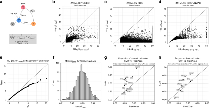
Fig. 5 Comparison between summary-PrediXcan and SMR. a Depicts how SMR tests the mediating role of gene expression level Tg. The top eQTL is linked to the phenotype as an instrumental variable in a Mendelian Randomization approach. b Shows the significance of SMR vs. the significance of Summary-PrediXcan. As expected, SMR associations tend to be smaller than S-PrediXcan ones. c and d show that the SMR statistics significance is bounded by GWAS and eQTL p-values. The p-values (−log10) of the SMR statistics are plotted against the GWAS p-value of the top eQTL SNP (c), and the gene’s top eQTL p-value (d). e Shows a QQ plot for simulated values of TSMR. Under the null hypothesis of significant eQTL signal and no GWAS association, we generated random values for ZGWAS² and ZeQTL² following the simulations from ref. 16. TSMR statistic was calculated from these values, and compared to a χ1² distribution to illustrate this statistics’ deflation. f shows the sample mean of TSMR from 1000 simulations, centered close to 0.93, instead of the expected value of 1 for a χ1²-distributed variable. g shows the proportion of non-colocalized significant associations to total significant associations in PrediXcan and SMR. h Shows the proportion of colocalized significant associations (shared eQTL and GWAS signals). As expected, SMR shows a higher proportion of colocalized and non-colocalized associations than PrediXcan. This is caused by SMR’s high eQTL significance threshold, that rules out most of the genes with low colocalization power (P0 + P1 + P2 > 0.5). For some of the associations, GWAS and eQTL p-values were more significant than shown since they were thresholded at 10−50 to improve visualization. Phenotype abbreviations are as follows: FNBD Femoral Neck Bone Density, LSBD Lumbar Spine Bone Density, BMI Body Mass Index, HEIGHT Height, LDL Low-Density Lipoprotein Cholesterol, HDL High-Density Lipoprotein Cholesterol, TRYG Tryglicerides, CROHN Crohn’s Disease, INFBOWEL Inflammatory Bowel’s Disease, ULCERC Ulcerative Colitis, HBA1C Hemogoblin Levels, HOMA-IR HOMA Insulin Response, SCZ Schizophrenia, RA Rheumatoid Arthritis, COLLEGE College Completion, EDUCYEARS Education Years
Fig. 5 Comparison between summary-PrediXcan and SMR. a Depicts how SMR tests the mediating role of gene expression level Tg. The top eQTL is linked to the phenotype as an instrumental variable in a Mendelian Randomization approach. b Shows the significance of SMR vs. the significance of Summary-PrediXcan. As expected, SMR associations tend to be smaller than S-PrediXcan ones. c and d show that the SMR statistics significance is bounded by GWAS and eQTL p-values. The p-values (−log10) of the SMR statistics are plotted against the GWAS p-value of the top eQTL SNP (c), and the gene’s top eQTL p-value (d). e Shows a QQ plot for simulated values of TSMR. Under the null hypothesis of significant eQTL signal and no GWAS association, we generated random values for ZGWAS² and ZeQTL² following the simulations from ref. 16. TSMR statistic was calculated from these values, and compared to a χ1² distribution to illustrate this statistics’ deflation. f shows the sample mean of TSMR from 1000 simulations, centered close to 0.93, instead of the expected value of 1 for a χ1²-distributed variable. g shows the proportion of non-colocalized significant associations to total significant associations in PrediXcan and SMR. h Shows the proportion of colocalized significant associations (shared eQTL and GWAS signals). As expected, SMR shows a higher proportion of colocalized and non-colocalized associations than PrediXcan. This is caused by SMR’s high eQTL significance threshold, that rules out most of the genes with low colocalization power (P0 + P1 + P2 > 0.5). For some of the associations, GWAS and eQTL p-values were more significant than shown since they were thresholded at 10−50 to improve visualization. Phenotype abbreviations are as follows: FNBD Femoral Neck Bone Density, LSBD Lumbar Spine Bone Density, BMI Body Mass Index, HEIGHT Height, LDL Low-Density Lipoprotein Cholesterol, HDL High-Density Lipoprotein Cholesterol, TRYG Tryglicerides, CROHN Crohn’s Disease, INFBOWEL Inflammatory Bowel’s Disease, ULCERC Ulcerative Colitis, HBA1C Hemogoblin Levels, HOMA-IR HOMA Insulin Response, SCZ Schizophrenia, RA Rheumatoid Arthritis, COLLEGE College Completion, EDUCYEARS Education YearsCC BY · PubMed Central
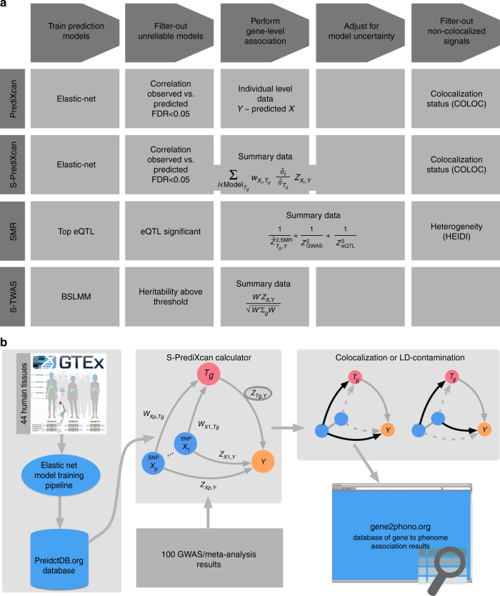
Fig. 6 MetaXcan framework and application. a Shows a general framework (MetaXcan) which encompasses methods such as PrediXcan, TWAS, SMR, COLOC among others. b Summarizes the application of the MetaXcan framework with S-PrediXcan using 44 GTEx tissue transcriptomes and over 100 GWAS and meta analysis results. We trained prediction models using elastic-net26 and deposited the weights and SNP covariances in the publicly available resource (http://predictdb.org/). The weights, covariances, and over 100 GWAS summary results were processed with S-PrediXcan. Colocalization status was computed and the full set of results was deposited in gene2pheno.org
Fig. 6 MetaXcan framework and application. a Shows a general framework (MetaXcan) which encompasses methods such as PrediXcan, TWAS, SMR, COLOC among others. b Summarizes the application of the MetaXcan framework with S-PrediXcan using 44 GTEx tissue transcriptomes and over 100 GWAS and meta analysis results. We trained prediction models using elastic-net26 and deposited the weights and SNP covariances in the publicly available resource (http://predictdb.org/). The weights, covariances, and over 100 GWAS summary results were processed with S-PrediXcan. Colocalization status was computed and the full set of results was deposited in gene2pheno.orgCC BY · PubMed Central
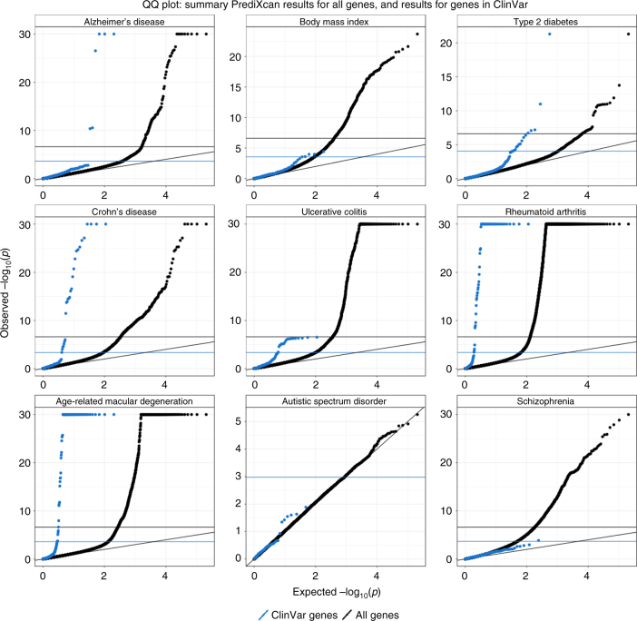
Fig. 7 ClinVar genes show significant S-PrediXcan associations. Genes implicated in ClinVar tended to be more significant in S-PrediXcan for most diseases tested, except for schizophrenia and autism. This suggests that more moderate alteration of monogenic disease genes may contribute in a continuum of more moderate but related phenotypes. Alternatively, a more complex interplay between common and rare variation could be taking place such as higher tolerance to loss of function mutations in lower expressing haplotypes which could induce association with predicted expression. Blue circles correspond to the QQ plot of genes in ClinVar that were annotated with the phenotype and black circles correspond to all genes
Fig. 7 ClinVar genes show significant S-PrediXcan associations. Genes implicated in ClinVar tended to be more significant in S-PrediXcan for most diseases tested, except for schizophrenia and autism. This suggests that more moderate alteration of monogenic disease genes may contribute in a continuum of more moderate but related phenotypes. Alternatively, a more complex interplay between common and rare variation could be taking place such as higher tolerance to loss of function mutations in lower expressing haplotypes which could induce association with predicted expression. Blue circles correspond to the QQ plot of genes in ClinVar that were annotated with the phenotype and black circles correspond to all genesCC BY · PubMed Central
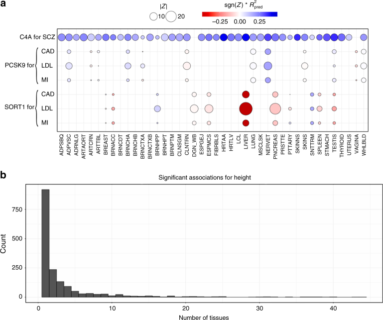
Fig. 8 S-PrediXcan associations in different tissues. a Displays associations for PCSK9, SORT1, and C4A on relevant traits by tissue. This figure shows the association strength between three well studied genes and corresponding phenotypes. C4A associations with schizophrenia (SCZ) are significant across most tissues. SORT1 associations with LDL-C, coronary artery disease (CAD), and myocardial infarction (MI) are most significant in liver. PCSK9 associations with LDL-C, coronary artery disease (CAD), and myocardial infarction (MI) are most significant in tibial nerve. The size of the points represent the significance of the association between predicted expression and the traits indicated on the top labels. Red indicates negative correlation whereas blue indicates positive correlation. Rpred² is a performance measure computed as the correlation squared between observed and predicted expression, cross validated in the training set. Darker points indicate larger genetic component and consequently more active regulation in the tissue. b Displays a histogram of the number of tissues for which a gene is significantly associated with height (other phenotypes show a similar pattern). Tissue abbreviations: ADPSBQ Adipose-Subcutaneous, ADPVSC Adipose-Visceral(Omentum), ADRNLG Adrenal Gland, ARTAORT Artery-Aorta, ARTCRN Artery-Coronary, ARTTBL Artery-Tibial, BLDDER Bladder, BRNAMY Brain-Amygdala, BRNACC Brain-Anterior cingulate cortex (BA24), BRNCDT Brain-Caudate(basal ganglia), BRNCHB Brain-Cerebellar Hemisphere, BRNCHA Brain-Cerebellum, BRNCTXA Brain-Cortex, BRNCTXB Brain-Frontal Cortex (BA9), BRNHPP Brain-Hippocampus, BRNHPT Brain-Hypothalamus, BRNNCC Brain Nucleus accumbens(basal ganglia), BRNPTM Brain-Putamen (basal ganglia), BRNSPC Brain-Spinal cord(cervical c-1), BRNSNG Brain-Substantia nigra, BREAST Breast-Mammary Tissue, LCL Cells-EBV-transformed lymphocytes, FIBRBLS Cells-Transformed fibroblasts, CVXECT Cervix-Ectocervix, CVSEND Cervix-Endocervix, CLNSGM Colon-Sigmoid, CLNTRN Colon-Transverse, ESPGEJ Esophagus-Gastroesophageal Junction, ESPMCS Esophagus-Mucosa, ESPMSL Esophagus-Muscularis, FLLPNT Fallopian Tube, HRTAA Heart-Atrial Appendage, HRTLV Heart-Left Ventricle, KDNCTX Kidney-Cortex, LIVER Liver, LUNG Lung, SLVRYG Minor Salivary Gland, MSCLSK Muscle-Skeletal, NERVET Nerve-Tibial, OVARY Ovary, PNCREAS Pancreas, PTTARY Pituitary, PRSTTE Prostate, SKINNS Skin-Not Sun Exposed (Suprapubic), SKINS Skin-Sun Exposed (Lower leg), SNTTRM Small Intestine-Terminal Ileum, SPLEEN Spleen, STMACH Stomach, TESTIS Testis, THYROID Thyroid, UTERUS Uterus, VAGINA Vagina, WHLBLD Whole Blood
Fig. 8 S-PrediXcan associations in different tissues. a Displays associations for PCSK9, SORT1, and C4A on relevant traits by tissue. This figure shows the association strength between three well studied genes and corresponding phenotypes. C4A associations with schizophrenia (SCZ) are significant across most tissues. SORT1 associations with LDL-C, coronary artery disease (CAD), and myocardial infarction (MI) are most significant in liver. PCSK9 associations with LDL-C, coronary artery disease (CAD), and myocardial infarction (MI) are most significant in tibial nerve. The size of the points represent the significance of the association between predicted expression and the traits indicated on the top labels. Red indicates negative correlation whereas blue indicates positive correlation. Rpred² is a performance measure computed as the correlation squared between observed and predicted expression, cross validated in the training set. Darker points indicate larger genetic component and consequently more active regulation in the tissue. b Displays a histogram of the number of tissues for which a gene is significantly associated with height (other phenotypes show a similar pattern). Tissue abbreviations: ADPSBQ Adipose-Subcutaneous, ADPVSC Adipose-Visceral(Omentum), ADRNLG Adrenal Gland, ARTAORT Artery-Aorta, ARTCRN Artery-Coronary, ARTTBL Artery-Tibial, BLDDER Bladder, BRNAMY Brain-Amygdala, BRNACC Brain-Anterior cingulate cortex (BA24), BRNCDT Brain-Caudate(basal ganglia), BRNCHB Brain-Cerebellar Hemisphere, BRNCHA Brain-Cerebellum, BRNCTXA Brain-Cortex, BRNCTXB Brain-Frontal Cortex (BA9), BRNHPP Brain-Hippocampus, BRNHPT Brain-Hypothalamus, BRNNCC Brain Nucleus accumbens(basal ganglia), BRNPTM Brain-Putamen (basal ganglia), BRNSPC Brain-Spinal cord(cervical c-1), BRNSNG Brain-Substantia nigra, BREAST Breast-Mammary Tissue, LCL Cells-EBV-transformed lymphocytes, FIBRBLS Cells-Transformed fibroblasts, CVXECT Cervix-Ectocervix, CVSEND Cervix-Endocervix, CLNSGM Colon-Sigmoid, CLNTRN Colon-Transverse, ESPGEJ Esophagus-Gastroesophageal Junction, ESPMCS Esophagus-Mucosa, ESPMSL Esophagus-Muscularis, FLLPNT Fallopian Tube, HRTAA Heart-Atrial Appendage, HRTLV Heart-Left Ventricle, KDNCTX Kidney-Cortex, LIVER Liver, LUNG Lung, SLVRYG Minor Salivary Gland, MSCLSK Muscle-Skeletal, NERVET Nerve-Tibial, OVARY Ovary, PNCREAS Pancreas, PTTARY Pituitary, PRSTTE Prostate, SKINNS Skin-Not Sun Exposed (Suprapubic), SKINS Skin-Sun Exposed (Lower leg), SNTTRM Small Intestine-Terminal Ileum, SPLEEN Spleen, STMACH Stomach, TESTIS Testis, THYROID Thyroid, UTERUS Uterus, VAGINA Vagina, WHLBLD Whole BloodCC BY · PubMed Central
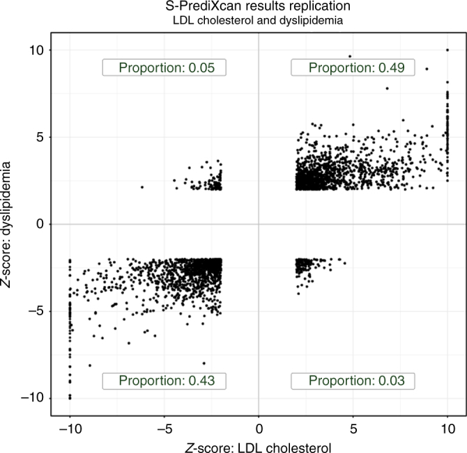
Fig. 9 Discovery and replication Z-scores for lipid trait. This figure shows the Z-scores of the association between dyslipidemia (GERA) and predicted gene expression levels on the vertical axis and the Z-scores for LDL cholesterol on the horizontal axis. To facilitate visualization, very large Z-scores where thresholded to 10. Proportions in each quadrant were computed excluding Z-scores with magnitude smaller than 2 to filter out noise
Fig. 9 Discovery and replication Z-scores for lipid trait. This figure shows the Z-scores of the association between dyslipidemia (GERA) and predicted gene expression levels on the vertical axis and the Z-scores for LDL cholesterol on the horizontal axis. To facilitate visualization, very large Z-scores where thresholded to 10. Proportions in each quadrant were computed excluding Z-scores with magnitude smaller than 2 to filter out noiseCC BY · PubMed Central

Verification

Claims the paper makes

The claims and statistics of this paper haven’t been checked yet.

Run the check — free, no account needed. It reads the open-access text and checks the sources it cites.

A few free checks a day · papers already verified open instantly · results are public

Claims other papers make about this one

Each is checked against this paper’s own text: does it say what the citing paper says it does?

Self-check

Percentages, sums and reported differences re-computed from the paper’s own numbers.

The self-check needs the paper’s full text.

Citations

Cites

Show all 50 references

Cited by

Sorted by citations

See all 69

Metadata

Authors
Barbeira, A. N., Dickinson, S. P., Bonazzola, R., Zheng, J., Wheeler, H. E., Torres, J. M., Torstenson, E. S., Shah, K. P., Garcia, T., Edwards, T. L., Stahl, E. A., Huckins, L. M., GTEx Consortium, Laboratory, D. A. &. C. C. (. W. G., Aguet, F., Ardlie, K. G., Cummings, B. B., Gelfand, E. T., Getz, G., Hadley, K., Handsaker, R. E., Huang, K. H., Kashin, S., Karczewski, K. J., Lek, M., Li, X., MacArthur, D. G., Nedzel, J. L., Nguyen, D. T., Noble, M. S., Segrè, A. V., Trowbridge, C. A., Tukiainen, T., Statistical Methods groups—Analysis Working Group, Abell, N. S., Balliu, B., Barshir, R., Basha, O., Battle, A., Bogu, G. K., Brown, A., Brown, C. D., Castel, S. E., Chen, L. S., Chiang, C., Conrad, D. F., Damani, F. N., Davis, J. R., Delaneau, O., Dermitzakis, E. T., Engelhardt, B. E., Eskin, E., Ferreira, P. G., Frésard, L., Gamazon, E. R., Garrido-Martín, D., Gewirtz, A. D. H., Gliner, G., Gloudemans, M. J., Guigo, R., Hall, I. M., Han, B., He, Y., Hormozdiari, F., Howald, C., Jo, B., Kang, E. Y., Kim, Y., Kim-Hellmuth, S., Lappalainen, T., Li, G., Li, X., Liu, B., Mangul, S., McCarthy, M. I., McDowell, I. C., Mohammadi, P., Monlong, J., Montgomery, S. B., Muñoz-Aguirre, M., Ndungu, A. W., Nobel, A. B., Oliva, M., Ongen, H., Palowitch, J. J., Panousis, N., Papasaikas, P., Park, Y., Parsana, P., Payne, A. J., Peterson, C. B., Quan, J., Reverter, F., Sabatti, C., Saha, A., Sammeth, M., Scott, A. J., Shabalin, A. A., Sodaei, R., Stephens, M., Stranger, B. E., Strober, B. J., Sul, J. H., Tsang, E. K., Urbut, S., van de Bunt, M., Wang, G., Wen, X., Wright, F. A., Xi, H. S., Yeger-Lotem, E., Zappala, Z., Zaugg, J. B., Zhou, Y.-H., groups, E. G. (., Akey, J. M., Bates, D., Chan, J., Chen, L. S., Claussnitzer, M., Demanelis, K., Diegel, M., Doherty, J. A., Feinberg, A. P., Fernando, M. S., Halow, J., Hansen, K. D., Haugen, E., Hickey, P. F., Hou, L., Jasmine, F., Jian, R., Jiang, L., Johnson, A., Kaul, R., Kellis, M., Kibriya, M. G., Lee, K., Li, J. B., Li, Q., Li, X., Lin, J., Lin, S., Linder, S., Linke, C., Liu, Y., Maurano, M. T., Molinie, B., Montgomery, S. B., Nelson, J., Neri, F. J., Oliva, M., Park, Y., Pierce, B. L., Rinaldi, N. J., Rizzardi, L. F., Sandstrom, R., Skol, A., Smith, K. S., Snyder, M. P., Stamatoyannopoulos, J., Stranger, B. E., Tang, H., Tsang, E. K., Wang, L., Wang, M., Van Wittenberghe, N., Wu, F., Zhang, R., Fund, N. C., Nierras, C. R., NIH/NCI, Branton, P. A., Carithers, L. J., Guan, P., Moore, H. M., Rao, A., Vaught, J. B., NIH/NHGrI, Gould, S. E., Lockart, N. C., Martin, C., Struewing, J. P., Volpi, S., NIH/NIMH, Addington, A. M., Koester, S. E., NIH/NIDA, Little, A. R., Site—NDrI, B. C. S., Brigham, L. E., Hasz, R., Hunter, M., Johns, C., Johnson, M., Kopen, G., Leinweber, W. F., Lonsdale, J. T., McDonald, A., Mestichelli, B., Myer, K., Roe, B., Salvatore, M., Shad, S., Thomas, J. A., Walters, G., Washington, M., Wheeler, J., Site—rPCI, B. C. S., Bridge, J., Foster, B. A., Gillard, B. M., Karasik, E., Kumar, R., Miklos, M., Moser, M. T., resource—VArI, B. C., Jewell, S. D., Montroy, R. G., Rohrer, D. C., Valley, D. R., Brain Bank repository—University of Miami Brain Endowment Bank, Davis, D. A., Mash, D. C., Leidos Biomedical—Project Management, Undale, A. H., Smith, A. M., Tabor, D. E., Roche, N. V., McLean, J. A., Vatanian, N., Robinson, K. L., Sobin, L., Barcus, M. E., Valentino, K. M., Qi, L., Hunter, S., Hariharan, P., Singh, S., Um, K. S., Matose, T., Tomaszewski, M. M., Study, E., Barker, L. K., Mosavel, M., Siminoff, L. A., Traino, H. M., Visualization—EBI, G. B. D. I. &., Flicek, P., Juettemann, T., Ruffier, M., Sheppard, D., Taylor, K., Trevanion, S. J., Zerbino, D. R., Genome Browser Data Integration & Visualization—UCSC Genomics Institute, U. O. C. S. C., Craft, B., Goldman, M., Haeussler, M., Kent, W. J., Lee, C. M., Paten, B., Rosenbloom, K. R., Vivian, J., Zhu, J., Nicolae, D. L., Cox, N. J., & Im, H. K.
Affiliations
  • University of Chicago (US)
  • Loyola University Chicago (US)
  • Vanderbilt University (US)
  • Vanderbilt University Medical Center (US)
  • Broad Institute (US)
  • Stanford University (US)
  • Ben-Gurion University of the Negev (IL)
  • Johns Hopkins University (US)
  • Universitat Pompeu Fabra (ES)
  • University of Geneva (CH)
  • University of Pennsylvania (US)
  • Columbia University Irving Medical Center (US)
  • Washington University in St. Louis (US)
  • Princeton University (US)
  • University of California, Los Angeles (US)
  • Universidade do Porto (PT)
  • Amsterdam UMC Location University of Amsterdam (NL)
  • Asan Medical Center (KR)
  • Columbia University (US)
  • Centre for Human Genetics (GB)
  • Duke University (US)
  • University of North Carolina at Chapel Hill (US)
  • The University of Texas MD Anderson Cancer Center (US)
  • Pfizer (United States) (US)
  • Universidade Federal do Rio de Janeiro (BR)
  • University of Utah (US)
  • University of Michigan (US)
  • North Carolina State University (US)
  • European Molecular Biology Laboratory (DE)
  • Altius Institute for Biomedical Sciences (US)
  • University of Washington (US)
  • NYU Langone Health (US)
  • National Institutes of Health (US)
  • National Cancer Institute (US)
  • National Institute of Dental and Craniofacial Research (US)
  • National Human Genome Research Institute (US)
  • Lifenet Health (US)
  • National Disease Research Interchange (US)
  • University at Buffalo, State University of New York (US)
  • Roswell Park Comprehensive Cancer Center (US)
  • Van Andel Institute (US)
  • University of Miami (US)
  • Leidos Biomedical Research Inc. (United States) (US)
  • Temple University (US)
  • Virginia Commonwealth University (US)
  • European Bioinformatics Institute (GB)
  • University of California, Santa Cruz (US)
Corresponding author
Im, Hae Kyung
ORCID
Venue
Nature Communications
Published
2018-05-08
Volume
9
Issue
1
Pages
1825-1825
ISSN
2041-1723 (ISSN-L)
OpenAlex
W2952346218
Cited by
69
References
50
Citations by year
2026: 16 · 2025: 3 · 2024: 4 · 2023: 2 · 2022: 1 · 2021: 6 · 2020: 2 · 2019: 10 · 2018: 16
FWCI
5.20
Type
journal article
Language
en
Open access
Locations
  • Nature Communications (publishedVersion, cc-by)
  • bioRxiv (Cold Spring Harbor Laboratory) (acceptedVersion, cc-by)
  • Europe PMC (PubMed Central) (publishedVersion, cc-by)
  • PubMed Central (publishedVersion, cc-by)
  • PubMed (publishedVersion)
  • Repositori digital de la UPF (Universitat Pompeu Fabra) (publishedVersion, cc-by)
  • Digital Access to Scholarship at Harvard (DASH) (Harvard University) (submittedVersion, cc-by)
  • Loyola eCommons (Loyola University of Chicago) (submittedVersion, cc-by)
  • RePEc: Research Papers in Economics (submittedVersion)
  • DOAJ (DOAJ: Directory of Open Access Journals) (submittedVersion, cc-by-sa)
  • DOAJ (DOAJ: Directory of Open Access Journals) (submittedVersion)
  • TUScholarShare (Temple University) (submittedVersion, cc-by)
  • RECERCAT (Consorci de Serveis Universitaris de Catalunya) (submittedVersion, cc-by)
  • Seoul National University Open Repository (Seoul National University) (submittedVersion)
Funders
  • University of Miami
  • University of Pennsylvania
  • Harvard University
  • Loyola University Chicago
  • Georgia Clinical and Translational Science Alliance (UL1 TR000430)
  • Université de Genève
  • National Institutes of Health (UL1TR000430, 5p50mh094267-05)
  • Medical Research Council (MR/N01104X/1)
  • National Heart, Lung, and Blood Institute
  • National Institute of Mental Health (R01MH101814, T32MH020065, R01MH101822, R01MH090937, R01MH107666, R01MH101810, R01MH101782, R01MH101819, R01MH101820, R01MH090948, R01MH101825, R01MH090941, R01MH090936, R01MH090951)
  • National Institute on Drug Abuse (R01DA033684, R01DA006227, P50DA037844)
  • National Human Genome Research Institute (R15HG009569)
  • NIH Office of the Director
  • National Cancer Institute
  • National Institute of Diabetes and Digestive and Kidney Diseases (F31DK101202, P30DK020595)
  • National Institute of Neurological Disorders and Stroke
  • Common Fund
Topics
  • Life Sciences › Biochemistry, Genetics and Molecular Biology › Genetics › Genetic Associations and Epidemiology
  • Life Sciences › Biochemistry, Genetics and Molecular Biology › Molecular Biology › Bioinformatics and Genomic Networks
  • Life Sciences › Biochemistry, Genetics and Molecular Biology › Genetics › Genetic Mapping and Diversity in Plants and Animals
Keywords
tissue-specific gene expression, expression quantitative trait loci, PrediXcan, GWAS summary statistics, GTEx, gene mapping, phenotypic association, colocalization
MeSH terms
Chromosome Mapping, Computer Simulation, Humans, Models, Genetic, Organ Specificity, Phenotype, Genetic Variation, Meta-Analysis as Topic, Gene Expression, Polymorphism, Single Nucleotide, Quantitative Trait Loci, Genome-Wide Association Study

About these checks

Registry, retraction, Cites and statistics results are computed, not judged, with one exception: a printed reference that no index lists is read once by a model before it counts as a citation error. Claims are extracted by a model and kept only when their quote appears verbatim in the text; each cited source is then checked, with a model’s help, for whether it says what the claim relies on. Those verdicts can be wrong — read the claim’s quote and the cited source before relying on one.

Statistics and arithmetic are recomputed, not judged.

Confidence bands are shown only for fields calibrated on our annotated test set. None is calibrated yet, so no band is shown.

What counts as a claim ›How we measure confidence ›How we check this ›

Are you an author, or do you see a problem with this page? Request a review