CoChat

Slide-tags enables single-nucleus barcoding for multimodal spatial genomics

Open access

The DOI matches its Crossref record; 99 of the 99 references it cites were found in a registry or an index.

Abstract

Recent technological innovations have enabled the high-throughput quantification of gene expression and epigenetic regulation within individual cells, transforming our understanding of how complex tissues are constructed 1–6. However, missing from these measurements is the ability to routinely and easily spatially localize these profiled cells. We developed a strategy, Slide-tags, in which single nuclei within an intact tissue section are tagged with spatial barcode oligonucleotides derived from DNA-barcoded beads with known positions. These tagged nuclei can then be used as an input into a wide variety of single-nucleus profiling assays. Application of Slide-tags to the mouse hippocampus positioned nuclei at less than 10 μm spatial resolution and delivered whole-transcriptome data that are indistinguishable in quality from ordinary single-nucleus RNA-sequencing data. To demonstrate that Slide-tags can be applied to a wide variety of human tissues, we performed the assay on brain, tonsil and melanoma. We revealed cell-type-specific spatially varying gene expression across cortical layers and spatially contextualized receptor–ligand interactions driving B cell maturation in lymphoid tissue. A major benefit of Slide-tags is that it is easily adaptable to almost any single-cell measurement technology. As a proof of principle, we performed multiomic measurements of open chromatin, RNA and T cell receptor (TCR) sequences in the same cells from metastatic melanoma, identifying transcription factor motifs driving cancer cell state transitions in spatially distinct microenvironments. Slide-tags offers a universal platform for importing the compendium of established single-cell measurements into the spatial genomics repertoire.

Overview

The claims and statistics of this paper haven’t been checked yet.

Free: it reads the open-access text and checks the first 5 claims that cite a source we can check. Create a free account to check every claim.

A few free checks a day · papers already verified open instantly · results are public

Integrity signals

Registry

Crossref · 10.1038/s41586-023-06837-4

Cites

99 of 99 references verified0 citation errors · 0 not checkable

Statistics

Figures

Fig. 1 Slide-tags enables single-nucleus spatial transcriptomics in the mouse hippocampus. a, Schematic of Slide-tags. A 20-μm fresh-frozen tissue section is applied to a monolayer of randomly deposited, DNA-barcoded beads that have been spatially indexed. These DNA spatial barcodes are photocleaved and associate with nuclei. Spatially barcoded nuclei are then profiled using established droplet-based single-nucleus sequencing technologies. The diagram was created using BioRender. b, Uniform manifold approximation and projection (UMAP) embedding of snRNA-seq profiles coloured by cell type annotations. DG, dentate gyrus; oligo, oligodendrocyte. c, The signal spatial barcode clusters after noise filtering by DBSCAN for selected cells, coloured according to cell type annotations (as in b) and the number of spatial barcode UMIs. Raw plots for these cells are plotted in Extended Data Fig. 2k. d, Slide-tags enables localization of nuclei to spatial coordinates in the mouse hippocampus; cells are coloured according to cell type annotation (as in b). e, Spatial expression of known marker genes compared with in situ hybridization data from the Allen Mouse Brain Atlas23. Colour scales, normalized average counts. f, The distance from the centroid for each of the spatial barcodes across all signal spatial barcode clusters; points are coloured by the two-dimensional kernel density estimation with an axis-aligned bivariate normal kernel, evaluated on a square grid. Kernel density estimates are displayed for x and y. For the plots on the outside, the centre lines show the median, and the adjacent lines show the upper and lower quartiles. g–i, Comparison metrics plotted for snRNA-seq compared with Slide-tags snRNA-seq, performed on consecutive sections. g, Cell type proportions and mean UMIs per cell are plotted by cell type. h, The normalized average UMI counts were determined per gene across all cells. i, Normalized average counts. Expression counts for each cell were divided by the total counts for that cell and multiplied by 10,000, this value + 1 was then natural-log transformed. r is the Pearson correlation coefficient. The error bands denote the 95% confidence intervals. For c–e, scale bars, 500 μm.
Fig. 1 Slide-tags enables single-nucleus spatial transcriptomics in the mouse hippocampus. a, Schematic of Slide-tags. A 20-μm fresh-frozen tissue section is applied to a monolayer of randomly deposited, DNA-barcoded beads that have been spatially indexed. These DNA spatial barcodes are photocleaved and associate with nuclei. Spatially barcoded nuclei are then profiled using established droplet-based single-nucleus sequencing technologies. The diagram was created using BioRender. b, Uniform manifold approximation and projection (UMAP) embedding of snRNA-seq profiles coloured by cell type annotations. DG, dentate gyrus; oligo, oligodendrocyte. c, The signal spatial barcode clusters after noise filtering by DBSCAN for selected cells, coloured according to cell type annotations (as in b) and the number of spatial barcode UMIs. Raw plots for these cells are plotted in Extended Data Fig. 2k. d, Slide-tags enables localization of nuclei to spatial coordinates in the mouse hippocampus; cells are coloured according to cell type annotation (as in b). e, Spatial expression of known marker genes compared with in situ hybridization data from the Allen Mouse Brain Atlas23. Colour scales, normalized average counts. f, The distance from the centroid for each of the spatial barcodes across all signal spatial barcode clusters; points are coloured by the two-dimensional kernel density estimation with an axis-aligned bivariate normal kernel, evaluated on a square grid. Kernel density estimates are displayed for x and y. For the plots on the outside, the centre lines show the median, and the adjacent lines show the upper and lower quartiles. g–i, Comparison metrics plotted for snRNA-seq compared with Slide-tags snRNA-seq, performed on consecutive sections. g, Cell type proportions and mean UMIs per cell are plotted by cell type. h, The normalized average UMI counts were determined per gene across all cells. i, Normalized average counts. Expression counts for each cell were divided by the total counts for that cell and multiplied by 10,000, this value + 1 was then natural-log transformed. r is the Pearson correlation coefficient. The error bands denote the 95% confidence intervals. For c–e, scale bars, 500 μm.CC BY · PubMed Central
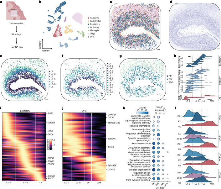
Fig. 2 Spatially resolved cell-type-specific expression in the human brain using Slide-tags snRNA-seq. a, Schematic of Slide-tags snRNA-seq analysis of a 10-mm square region of the human prefrontal cortex. Scale bar, 10 mm. The diagram was created using BioRender. b, UMAP embedding of snRNA-seq profiles, coloured according to cell type assignment. c, Spatial mapping of snRNA-seq profiles, coloured by cell type as in b. d, A Nissl-stained tissue section adjacent to the profiled section. e, Spatial mapping of grouped excitatory neuron subtypes. L1–6, cortical layers 1–6. f, Spatial mapping of grouped inhibitory neuron subtypes. g, Spatial mapping of astrocyte (AS) subtypes. GM, grey matter; PP, protoplasmic; WM, white matter. h, The layer specificity of grouped excitatory neuron, grouped inhibitory neuron and AS subtypes. i,j Heat maps of one-dimensional gene expression for excitatory neurons (i) and OPCs (j). k, Gene Ontology analysis of the highest spatially variable genes in each cell type. EX, excitatory; INH, inhibitory; Padj, adjusted P value. l, The spatial expression of genes with contrasting gradients across cell types. For c–g, scale bars, 500 μm.
Fig. 2 Spatially resolved cell-type-specific expression in the human brain using Slide-tags snRNA-seq. a, Schematic of Slide-tags snRNA-seq analysis of a 10-mm square region of the human prefrontal cortex. Scale bar, 10 mm. The diagram was created using BioRender. b, UMAP embedding of snRNA-seq profiles, coloured according to cell type assignment. c, Spatial mapping of snRNA-seq profiles, coloured by cell type as in b. d, A Nissl-stained tissue section adjacent to the profiled section. e, Spatial mapping of grouped excitatory neuron subtypes. L1–6, cortical layers 1–6. f, Spatial mapping of grouped inhibitory neuron subtypes. g, Spatial mapping of astrocyte (AS) subtypes. GM, grey matter; PP, protoplasmic; WM, white matter. h, The layer specificity of grouped excitatory neuron, grouped inhibitory neuron and AS subtypes. i,j Heat maps of one-dimensional gene expression for excitatory neurons (i) and OPCs (j). k, Gene Ontology analysis of the highest spatially variable genes in each cell type. EX, excitatory; INH, inhibitory; Padj, adjusted P value. l, The spatial expression of genes with contrasting gradients across cell types. For c–g, scale bars, 500 μm.CC BY · PubMed Central
Fig. 3 Slide-tags enables cell-type-specific spatially varying gene expression analysis and spatial receptor–ligand interaction prediction within the human tonsil. a, Schematic of Slide-tags snRNA-seq analysis of a 3-mm-diameter region of human tonsil tissue. Scale bar, 3 mm. The diagram was created using BioRender. b, UMAP embedding of snRNA-seq profiles coloured by cell type annotations. mDC, myeloid dendritic cells; pDC, plasmacytoid dendritic cells; TFH cells, T follicular helper cells. c, Spatial mapping of snRNA-seq profiles, coloured by cell type as in b. d, Adjacent haematoxylin and eosin (H&E)-stained section of the profiled region. e, Magnified view of two germinal centres coloured by cell type. f, Expression of dark-zone and light-zone marker genes identified as spatially varying within germinal centres. g, GCB cell state classification and zone segmentation on the basis of the cluster density of dark-zone GCB cells. h, Spatial mapping of TFH cells and follicular dendritic cells on zoned germinal centres. i, Selected spatially co-occurring receptor–ligand interactions within certain sender–receiver cell type pairs. j, Spatial mapping of interaction intensity scores for CD40 in GCB cells and CD40LG in TFH cells. For c–h and j, scale bars, 500 μm.
Fig. 3 Slide-tags enables cell-type-specific spatially varying gene expression analysis and spatial receptor–ligand interaction prediction within the human tonsil. a, Schematic of Slide-tags snRNA-seq analysis of a 3-mm-diameter region of human tonsil tissue. Scale bar, 3 mm. The diagram was created using BioRender. b, UMAP embedding of snRNA-seq profiles coloured by cell type annotations. mDC, myeloid dendritic cells; pDC, plasmacytoid dendritic cells; TFH cells, T follicular helper cells. c, Spatial mapping of snRNA-seq profiles, coloured by cell type as in b. d, Adjacent haematoxylin and eosin (H&E)-stained section of the profiled region. e, Magnified view of two germinal centres coloured by cell type. f, Expression of dark-zone and light-zone marker genes identified as spatially varying within germinal centres. g, GCB cell state classification and zone segmentation on the basis of the cluster density of dark-zone GCB cells. h, Spatial mapping of TFH cells and follicular dendritic cells on zoned germinal centres. i, Selected spatially co-occurring receptor–ligand interactions within certain sender–receiver cell type pairs. j, Spatial mapping of interaction intensity scores for CD40 in GCB cells and CD40LG in TFH cells. For c–h and j, scale bars, 500 μm.CC BY · PubMed Central
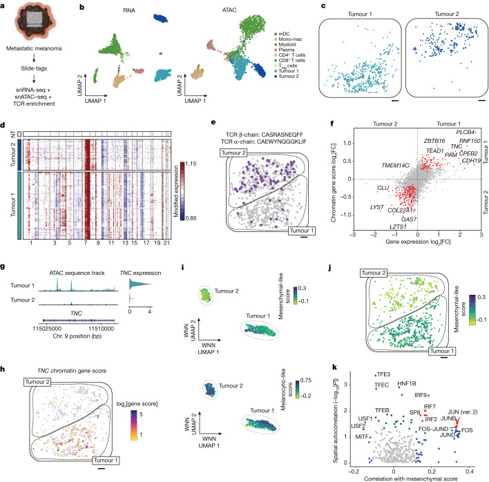
Fig. 4 Multiomic Slide-tags captures spatially resolved clonal relationships between single nuclei in human melanoma. a, Schematic of joint snATAC–seq and snRNA-seq analysis of a 5.5-mm square region of a human melanoma lymph node metastasis. Scale bar, 5.5 mm. The diagram was created using BioRender. b, UMAP embeddings of snRNA-seq and snATAC–seq profiles coloured by cell type. Mono-mac, monocyte-derived macrophages, Treg cells, regulatory T cells. c, Spatial mapping of tumour cluster 1 and tumour cluster 2. d, Inferred copy-number alterations from transcriptomic data. NT, a representative subset of non-tumour cells. e, Spatial mapping of a TCR β-chain clonotype expanded in the tumour cluster 2 compartment, with the matched α-chain indicated above. Grey cells show the positions of all CD8+ T cells. f, Differential gene expression and differential chromatin gene scores between tumour cluster 1 and tumour cluster 2. The red points have Padj < 0.05 for both tests. g, Genome coverage track and gene expression violin plot of TNC between tumour clusters. The range of the normalized chromatin accessibility signal is 0–50. Chr., chromosome. h, The spatial distribution of TNC chromatin accessibility gene scores. Gene scores are log2-transformed. i, Weighted nearest-neighbour (WNN) UMAP embedding of tumour cells, with cells coloured according to mesenchymal-like and melanocytic-like cell state scores. j, Spatial mapping of mesenchymal-like cell state scores in tumour cells. k, Spatial autocorrelation of accessibility in chromVAR transcription factor motifs correlated with mesenchymal-like cell state scores. The red points indicate spatial autocorrelation Moran’s I raw P < 0.05 and significant correlation with mesenchymal-like score (Padj < 0.05). The green points indicate only spatial autocorrelation raw P < 0.05. The blue points indicate only significant correlation with mesenchymal-like score (Padj < 0.05). Only chromVAR transcription factor motifs with a positive Moran’s I are shown. For c, e, h and j, scale bars, 500 μm.
Fig. 4 Multiomic Slide-tags captures spatially resolved clonal relationships between single nuclei in human melanoma. a, Schematic of joint snATAC–seq and snRNA-seq analysis of a 5.5-mm square region of a human melanoma lymph node metastasis. Scale bar, 5.5 mm. The diagram was created using BioRender. b, UMAP embeddings of snRNA-seq and snATAC–seq profiles coloured by cell type. Mono-mac, monocyte-derived macrophages, Treg cells, regulatory T cells. c, Spatial mapping of tumour cluster 1 and tumour cluster 2. d, Inferred copy-number alterations from transcriptomic data. NT, a representative subset of non-tumour cells. e, Spatial mapping of a TCR β-chain clonotype expanded in the tumour cluster 2 compartment, with the matched α-chain indicated above. Grey cells show the positions of all CD8+ T cells. f, Differential gene expression and differential chromatin gene scores between tumour cluster 1 and tumour cluster 2. The red points have Padj < 0.05 for both tests. g, Genome coverage track and gene expression violin plot of TNC between tumour clusters. The range of the normalized chromatin accessibility signal is 0–50. Chr., chromosome. h, The spatial distribution of TNC chromatin accessibility gene scores. Gene scores are log2-transformed. i, Weighted nearest-neighbour (WNN) UMAP embedding of tumour cells, with cells coloured according to mesenchymal-like and melanocytic-like cell state scores. j, Spatial mapping of mesenchymal-like cell state scores in tumour cells. k, Spatial autocorrelation of accessibility in chromVAR transcription factor motifs correlated with mesenchymal-like cell state scores. The red points indicate spatial autocorrelation Moran’s I raw P < 0.05 and significant correlation with mesenchymal-like score (Padj < 0.05). The green points indicate only spatial autocorrelation raw P < 0.05. The blue points indicate only significant correlation with mesenchymal-like score (Padj < 0.05). Only chromVAR transcription factor motifs with a positive Moran’s I are shown. For c, e, h and j, scale bars, 500 μm.CC BY · PubMed Central
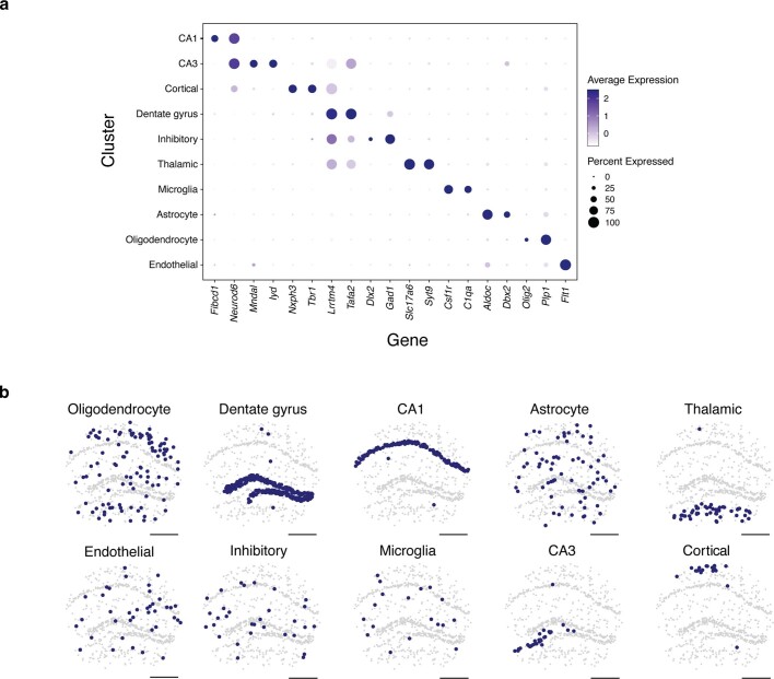
Extended Data Fig. 1 Cell type assignment and spatial mapping in the mouse hippocampus. a, Expression of marker genes by cell type cluster. b, Spatial positions of each cell by cell type cluster. All scale bars denote 500 μm. CA1 = Cornu Ammonis area 1, CA3 = Cornu Ammonis area 3. n = 839 nuclei.
Extended Data Fig. 1 Cell type assignment and spatial mapping in the mouse hippocampus. a, Expression of marker genes by cell type cluster. b, Spatial positions of each cell by cell type cluster. All scale bars denote 500 μm. CA1 = Cornu Ammonis area 1, CA3 = Cornu Ammonis area 3. n = 839 nuclei.CC BY · PubMed Central
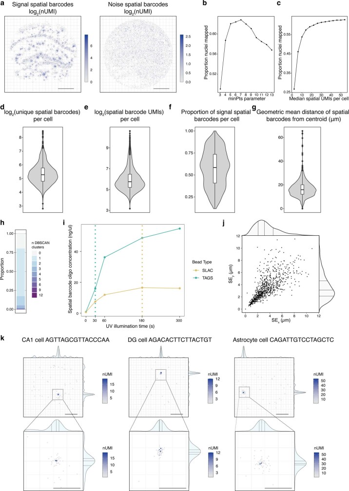
Extended Data Fig. 2 Assessing the mapping of single nuclei using spatial barcodes in the mouse hippocampus. a, Each recovered signal and noise spatial barcode is shown coloured by the number of detected UMIs. b, The proportion of nuclei mapped for each minPts parameter tested in DBSCAN. c, The proportion of nuclei mapped at different median spatial barcode nUMIs per cell. d-e, Violin plots showing different spatial barcode metrics for every cell that is a spatial singlet. f, Violin plot showing the proportion of spatial barcode UMIs that are assigned to the DBSCAN singlet cluster (signal) vs. all other spatial barcode UMIs recovered for that cell. g, Violin plot showing the mean radial distance for spatial barcodes for each spatial singlet cluster. h, The proportion of cells that are assigned to each number of DBSCAN clusters. i, plot showing the concentration of oligos released by time under illumination at the same light source power, for each bead type used in Slide-tags experiments. The time used for cleavage for each bead type is shown with the dotted lines. j, Plot showing the standard error (SE) for each singlet true spatial barcode cluster in x and y. Density shows: centre line, median; adjacent lines, upper and lower quartiles. k, The full set of spatial barcodes recovered for each of the nuclei plotted in Fig. 1c, with their xy positions, kernel density estimates, and coloured by nUMI associated with each cell are plotted (top). Points centred around the signal cluster are shown at higher magnification with final cell position shown as a cross (bottom). Scale bars denotes 500 μm, except for magnified plots, where scale bars denote 200 μm. Boxplots show: centre line, median; box limits, upper and lower quartiles; whiskers, 1.5x interquartile range; points, outliers. CA1 = Cornu Ammonis area 1, DG = dentate gyrus. a,j, n = 839 nuclei. d-g, n = 1042 nuclei. b,c,h, n = 1889 nuclei.
Extended Data Fig. 2 Assessing the mapping of single nuclei using spatial barcodes in the mouse hippocampus. a, Each recovered signal and noise spatial barcode is shown coloured by the number of detected UMIs. b, The proportion of nuclei mapped for each minPts parameter tested in DBSCAN. c, The proportion of nuclei mapped at different median spatial barcode nUMIs per cell. d-e, Violin plots showing different spatial barcode metrics for every cell that is a spatial singlet. f, Violin plot showing the proportion of spatial barcode UMIs that are assigned to the DBSCAN singlet cluster (signal) vs. all other spatial barcode UMIs recovered for that cell. g, Violin plot showing the mean radial distance for spatial barcodes for each spatial singlet cluster. h, The proportion of cells that are assigned to each number of DBSCAN clusters. i, plot showing the concentration of oligos released by time under illumination at the same light source power, for each bead type used in Slide-tags experiments. The time used for cleavage for each bead type is shown with the dotted lines. j, Plot showing the standard error (SE) for each singlet true spatial barcode cluster in x and y. Density shows: centre line, median; adjacent lines, upper and lower quartiles. k, The full set of spatial barcodes recovered for each of the nuclei plotted in Fig. 1c, with their xy positions, kernel density estimates, and coloured by nUMI associated with each cell are plotted (top). Points centred around the signal cluster are shown at higher magnification with final cell position shown as a cross (bottom). Scale bars denotes 500 μm, except for magnified plots, where scale bars denote 200 μm. Boxplots show: centre line, median; box limits, upper and lower quartiles; whiskers, 1.5x interquartile range; points, outliers. CA1 = Cornu Ammonis area 1, DG = dentate gyrus. a,j, n = 839 nuclei. d-g, n = 1042 nuclei. b,c,h, n = 1889 nuclei.CC BY · PubMed Central
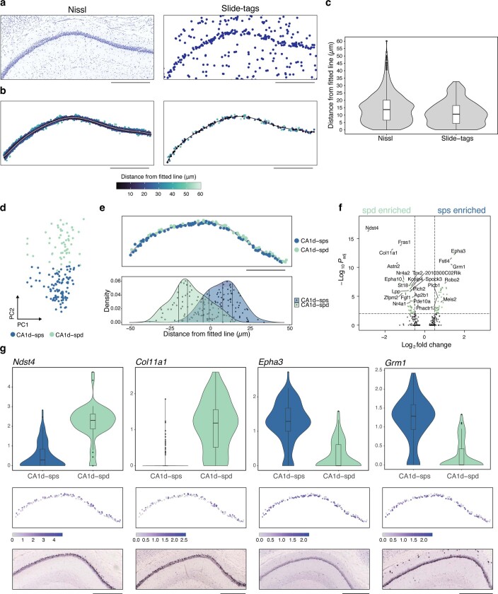
Extended Data Fig. 3 Spatial resolution measurements in the mouse hippocampus and Slide-tags snRNA-seq enables characterization of the deep and superficial sublayers in the mouse hippocampal CA1 field. a, A 10 um nissl-stained section (left) was taken adjacently to the Slide-tags profiled section (right). b, The CA1 nuclei were subsetted in each case and a line was fitted to measure the midpoint of this structure. For Slide-tags, nuclei were selected based on their cell type assignment in Figure S1, with 2 spatial outliers removed. For Nissl, nuclei were computationally segmented. Orthogonal distances from this midpoint were then calculated and points are coloured by this distance. c, Violin plots showing the distribution of distances from the fitted line in b. d, PCA plot showing cells from the CA1 cluster after subsetting, reprojection, and reclustering. Cells are coloured according to their new sub-cluster assignment. e, Cells from a are plotted according to their spatial location (top). The spatial density of nuclei from each population is plotted (bottom). f, Volcano plot showing differentially expressed genes between sps and spd. g, Violin plots showing gene expression differences between each subcluster (top) and the expression of these genes spatially (middle), as well as in situ hybridization data (bottom) from Allen Mouse Brain Atlas23. Genes were selected based on being discovered as differentially expressed between these two sub-clusters in our dataset and also identified in previous studies as defining these two sub-layers68,69. Boxplots show: centre line, median; box limits, upper and lower quartiles; whiskers, 1.5x interquartile range; points, outliers. All scale bars denote 500 μm. For Slide-tags CA1, n = 155 nuclei. For imaging data, n = 898 segmented nuclei.
Extended Data Fig. 3 Spatial resolution measurements in the mouse hippocampus and Slide-tags snRNA-seq enables characterization of the deep and superficial sublayers in the mouse hippocampal CA1 field. a, A 10 um nissl-stained section (left) was taken adjacently to the Slide-tags profiled section (right). b, The CA1 nuclei were subsetted in each case and a line was fitted to measure the midpoint of this structure. For Slide-tags, nuclei were selected based on their cell type assignment in Figure S1, with 2 spatial outliers removed. For Nissl, nuclei were computationally segmented. Orthogonal distances from this midpoint were then calculated and points are coloured by this distance. c, Violin plots showing the distribution of distances from the fitted line in b. d, PCA plot showing cells from the CA1 cluster after subsetting, reprojection, and reclustering. Cells are coloured according to their new sub-cluster assignment. e, Cells from a are plotted according to their spatial location (top). The spatial density of nuclei from each population is plotted (bottom). f, Volcano plot showing differentially expressed genes between sps and spd. g, Violin plots showing gene expression differences between each subcluster (top) and the expression of these genes spatially (middle), as well as in situ hybridization data (bottom) from Allen Mouse Brain Atlas23. Genes were selected based on being discovered as differentially expressed between these two sub-clusters in our dataset and also identified in previous studies as defining these two sub-layers68,69. Boxplots show: centre line, median; box limits, upper and lower quartiles; whiskers, 1.5x interquartile range; points, outliers. All scale bars denote 500 μm. For Slide-tags CA1, n = 155 nuclei. For imaging data, n = 898 segmented nuclei.CC BY · PubMed Central
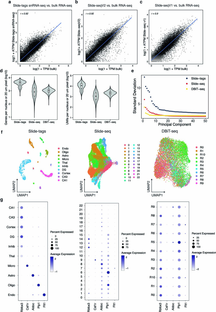
Extended Data Fig. 4 Comparison of Slide-tags to Bulk RNA-seq, Slide-seqV2 and DBiT-seq. a, Slide-tags snRNA-seq vs. bulk RNA-seq. b, Slide-seqV2 vs. bulkRNA-seq. c, Slide-seqV1 vs. bulkRNA-seq. Log10 transformations are shown in each bulk comparison case. d, Violin plots of log10-transformed genes and UMIs per nucleus (Slide-tags) or 20 μm spatial spot (Slide-seqV2 and DBiT-seq / spatial-ATAC-RNA-seq) in the mouse brain. n = 839 nuclei for Slide-tags, n = 18,950 20 μm pixels for Slide-seq, and n = 9,215 pixels for DBiT-seq. e, Elbow plot of standard deviations of principal components from Slide-tags snRNA-seq, Slide-seqV2, and DBiT-seq in the mouse brain. f, UMAP embeddings of snRNA-seq profiles from Slide-tags snRNA-seq (cell type labels), Slide-seqV2 (de novo clusters), and DBiT-seq (RNA clusters from Zhang et al.13) in the mouse brain. g, Dotplot expression of select markers across transcriptome clusters from Slide-tags snRNA-seq, Slide-seqV2, and DBiT-seq in the mouse brain. Boxplots show: centre line, median; box limits, upper and lower quartiles; whiskers, 1.5x interquartile range; points, outliers.
Extended Data Fig. 4 Comparison of Slide-tags to Bulk RNA-seq, Slide-seqV2 and DBiT-seq. a, Slide-tags snRNA-seq vs. bulk RNA-seq. b, Slide-seqV2 vs. bulkRNA-seq. c, Slide-seqV1 vs. bulkRNA-seq. Log10 transformations are shown in each bulk comparison case. d, Violin plots of log10-transformed genes and UMIs per nucleus (Slide-tags) or 20 μm spatial spot (Slide-seqV2 and DBiT-seq / spatial-ATAC-RNA-seq) in the mouse brain. n = 839 nuclei for Slide-tags, n = 18,950 20 μm pixels for Slide-seq, and n = 9,215 pixels for DBiT-seq. e, Elbow plot of standard deviations of principal components from Slide-tags snRNA-seq, Slide-seqV2, and DBiT-seq in the mouse brain. f, UMAP embeddings of snRNA-seq profiles from Slide-tags snRNA-seq (cell type labels), Slide-seqV2 (de novo clusters), and DBiT-seq (RNA clusters from Zhang et al.13) in the mouse brain. g, Dotplot expression of select markers across transcriptome clusters from Slide-tags snRNA-seq, Slide-seqV2, and DBiT-seq in the mouse brain. Boxplots show: centre line, median; box limits, upper and lower quartiles; whiskers, 1.5x interquartile range; points, outliers.CC BY · PubMed Central
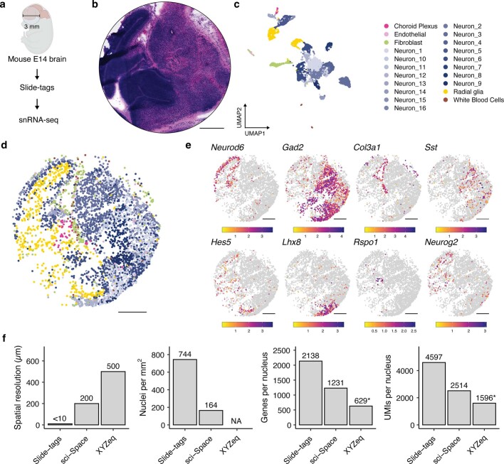
Extended Data Fig. 5 Slide-tags snRNA-seq applied to the embryonic mouse brain at E14. a, Schematic of Slide-tags snRNA-seq on a 3 mm diameter region of the embryonic mouse brain at E14. b. A haematoxylin and eosin stained section which was adjacent to the profiled section. c. UMAP embedding of snRNA-seq profiles coloured by cell-type annotations. d. Spatial positions of cells coloured as in C. e. Spatial marker gene expression. Expression counts for each cell were divided by the total counts for that cell and multiplied by 10,000, this value + 1 is then natural-log transformed. f. Comparison metrics plotted for Slide-tags snRNA-seq on the mouse E14 embryonic brain. * = XYZeq was not performed on embryonic mouse brain at E14 and so these metrics may not be directly comparable due to tissue-specific effects. All scale bars denote 500 μm.
Extended Data Fig. 5 Slide-tags snRNA-seq applied to the embryonic mouse brain at E14. a, Schematic of Slide-tags snRNA-seq on a 3 mm diameter region of the embryonic mouse brain at E14. b. A haematoxylin and eosin stained section which was adjacent to the profiled section. c. UMAP embedding of snRNA-seq profiles coloured by cell-type annotations. d. Spatial positions of cells coloured as in C. e. Spatial marker gene expression. Expression counts for each cell were divided by the total counts for that cell and multiplied by 10,000, this value + 1 is then natural-log transformed. f. Comparison metrics plotted for Slide-tags snRNA-seq on the mouse E14 embryonic brain. * = XYZeq was not performed on embryonic mouse brain at E14 and so these metrics may not be directly comparable due to tissue-specific effects. All scale bars denote 500 μm.CC BY · PubMed Central
Extended Data Fig. 6 Slide-tags snRNA-seq applied to the human brain enables spatial mapping of cell types and cell-type specific spatially varying gene expression. a, Individual plots of per-cell type spatial distribution. The diagram was created using BioRender. b, Dotplot showing the marker genes used to assign cell types to clusters. c, The gene expression distribution of four canonical layer marker genes in excitatory neurons. d,e, A 1D gene expression heatmap for genes in inhibitory neurons and astrocytes. All scale bars represent 500 µm. Oligo = Oligodendrocyte, OPC = Oligodendrocyte precursor cell, Astro = Astrocyte, Endo = Endothelial, WM = White matter. Gene names and details in Supplementary Table 2.
Extended Data Fig. 6 Slide-tags snRNA-seq applied to the human brain enables spatial mapping of cell types and cell-type specific spatially varying gene expression. a, Individual plots of per-cell type spatial distribution. The diagram was created using BioRender. b, Dotplot showing the marker genes used to assign cell types to clusters. c, The gene expression distribution of four canonical layer marker genes in excitatory neurons. d,e, A 1D gene expression heatmap for genes in inhibitory neurons and astrocytes. All scale bars represent 500 µm. Oligo = Oligodendrocyte, OPC = Oligodendrocyte precursor cell, Astro = Astrocyte, Endo = Endothelial, WM = White matter. Gene names and details in Supplementary Table 2.CC BY · PubMed Central
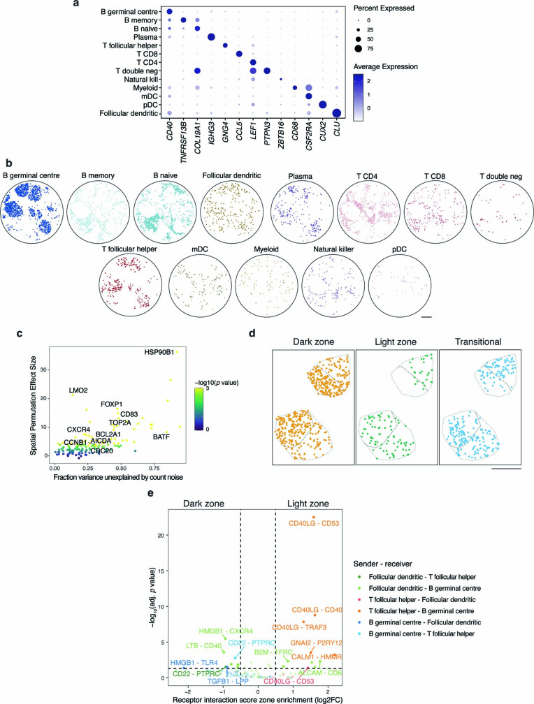
Extended Data Fig. 7 Receptor-ligand prediction from Slide-tags human tonsil data. a, Expression of select marker genes by cell type cluster. b, Spatial mapping of cell types. c, Scatter plot of gene expression variance not explained by count noise and spatial permutation effect size of previously reported dark zone and light zone marker genes. d, Spatial mapping of dark zone, light zone, and transitional germinal centre B cells in two representative germinal centres. e, Volcano plot of receptor interaction intensity scores compared between zones in two representative germinal centres. All scale bars denote 500 μm. T double neg = T double negative, mDC = myeloid dendritic cells, pDC = plasmacytoid dendritic cells.
Extended Data Fig. 7 Receptor-ligand prediction from Slide-tags human tonsil data. a, Expression of select marker genes by cell type cluster. b, Spatial mapping of cell types. c, Scatter plot of gene expression variance not explained by count noise and spatial permutation effect size of previously reported dark zone and light zone marker genes. d, Spatial mapping of dark zone, light zone, and transitional germinal centre B cells in two representative germinal centres. e, Volcano plot of receptor interaction intensity scores compared between zones in two representative germinal centres. All scale bars denote 500 μm. T double neg = T double negative, mDC = myeloid dendritic cells, pDC = plasmacytoid dendritic cells.CC BY · PubMed Central
Extended Data Fig. 8 Slide-tags snRNA-seq on human melanoma. a, Schematic representation of Slide-tags snRNA-seq and Slide-tags multiome (Fig. 4) profiled regions across tumour 1 and 2 compartments. b, UMAP embeddings of snRNA-seq profiles coloured by cell type. c, Spatial mapping of cell types. d, Spatial mapping of profiled cell types. e, Expression of select cell type marker genes and melanoma cell state marker genes. f, Inferred copy number alterations from transcriptomic data. NT indicates a representative subset of non-tumour cells. All scale bars denote 500 μm. T reg = T regulatory cells, mDC = myeloid dendritic cells, Mono-mac = monocyte-derived macrophages, pDC = plasmacytoid dendritic cells.
Extended Data Fig. 8 Slide-tags snRNA-seq on human melanoma. a, Schematic representation of Slide-tags snRNA-seq and Slide-tags multiome (Fig. 4) profiled regions across tumour 1 and 2 compartments. b, UMAP embeddings of snRNA-seq profiles coloured by cell type. c, Spatial mapping of cell types. d, Spatial mapping of profiled cell types. e, Expression of select cell type marker genes and melanoma cell state marker genes. f, Inferred copy number alterations from transcriptomic data. NT indicates a representative subset of non-tumour cells. All scale bars denote 500 μm. T reg = T regulatory cells, mDC = myeloid dendritic cells, Mono-mac = monocyte-derived macrophages, pDC = plasmacytoid dendritic cells.CC BY · PubMed Central
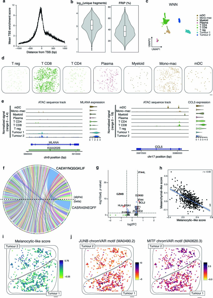
Extended Data Fig. 9 Slide-tags multiome on human melanoma. a, Mean TSS enrichment score. b, Violin plots of log10-transformed unique fragments and fraction of reads in peaks (FRiP) percentage. n = 2,529 nuclei. Boxplots show: centre line, median; box limits, upper and lower quartiles; whiskers, 1.5x interquartile range; points, outliers. c, Weighted nearest neighbour UMAP embeddings of snRNA-seq and snATAC-seq profiles coloured by cell type. d, Spatial mapping of cell types. e, ATAC sequence track and gene expression violin plot of MLANA and CCL5 across cell types. f, TCR pairing chord plot of alpha and beta chain pairing frequencies in CD8 T cells. g, Differential gene expression volcano plot between CD8 T cells in tumour compartment 1 vs tumour compartment 2. h, Scatter plot of melanocytic-like scores and mesenchymal-like scores of tumour cluster 1 cells in tumour compartment 1. Pearson’s r value is reported. Error band represents the 95% confidence interval. i, Mesenchymal-like cell state score spatial distribution. j, Spatial distribution of JUNB and MITF chromVAR motif scores. All scale bars denote 500 μm. T reg = T regulatory cells, mDC = myeloid dendritic cells, Mono-mac = monocyte-derived macrophages.
Extended Data Fig. 9 Slide-tags multiome on human melanoma. a, Mean TSS enrichment score. b, Violin plots of log10-transformed unique fragments and fraction of reads in peaks (FRiP) percentage. n = 2,529 nuclei. Boxplots show: centre line, median; box limits, upper and lower quartiles; whiskers, 1.5x interquartile range; points, outliers. c, Weighted nearest neighbour UMAP embeddings of snRNA-seq and snATAC-seq profiles coloured by cell type. d, Spatial mapping of cell types. e, ATAC sequence track and gene expression violin plot of MLANA and CCL5 across cell types. f, TCR pairing chord plot of alpha and beta chain pairing frequencies in CD8 T cells. g, Differential gene expression volcano plot between CD8 T cells in tumour compartment 1 vs tumour compartment 2. h, Scatter plot of melanocytic-like scores and mesenchymal-like scores of tumour cluster 1 cells in tumour compartment 1. Pearson’s r value is reported. Error band represents the 95% confidence interval. i, Mesenchymal-like cell state score spatial distribution. j, Spatial distribution of JUNB and MITF chromVAR motif scores. All scale bars denote 500 μm. T reg = T regulatory cells, mDC = myeloid dendritic cells, Mono-mac = monocyte-derived macrophages.CC BY · PubMed Central
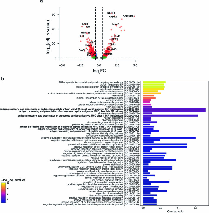
Extended Data Fig. 10 Differential gene expression and gene set enrichment analysis between tumour cluster 1 and 2. a, Volcano plot of differentially expressed genes comparing tumour cluster 1 against tumour cluster 2 from the Slide-tags snRNA-seq run. b, Gene ontology biological process (GO_Biological_Process_2021) gene set enrichment analysis on genes upregulated in tumour cluster 2 (negative log2FC) compared with tumour cluster 1 from the Slide-tags snRNA-seq experiment.
Extended Data Fig. 10 Differential gene expression and gene set enrichment analysis between tumour cluster 1 and 2. a, Volcano plot of differentially expressed genes comparing tumour cluster 1 against tumour cluster 2 from the Slide-tags snRNA-seq run. b, Gene ontology biological process (GO_Biological_Process_2021) gene set enrichment analysis on genes upregulated in tumour cluster 2 (negative log2FC) compared with tumour cluster 1 from the Slide-tags snRNA-seq experiment.CC BY · PubMed Central

Verification

Claims the paper makes

The claims and statistics of this paper haven’t been checked yet.

Free: it reads the open-access text and checks the first 5 claims that cite a source we can check. Create a free account to check every claim.

A few free checks a day · papers already verified open instantly · results are public

Claims other papers make about this one

Each is checked against this paper’s own text: does it say what the citing paper says it does?

Self-check

Percentages, sums and reported differences re-computed from the paper’s own numbers.

The self-check needs the paper’s full text.

Citations

Cites

Show all 99 references

Research works printed but not linked: 2

  1. Xu, X., Ester, M., Kriegel, H.-P. & Sander, J. A distribution-based clustering algorithm for mining in large spatial databases. In Proc. 14th International Conference on Data Engineering 324–331 (IEEE, 1998).
  2. Ester, M., Kriegel, H.-P., Sander, J. & Xu, X. A density-based algorithm for discovering clusters in large spatial databases with noise. In Proc. Second International Conference on Knowledge Discovery and Data Mining (eds Simoudis, E. et al.) 226–231 (AAAI Press, 1996).

Cited by

See all 225

Metadata

Authors
Russell, A. J. C., Weir, J. A., Nadaf, N. M., Shabet, M., Kumar, V., Kambhampati, S., Raichur, R., Marrero, G. J., Liu, S., Balderrama, K. S., Vanderburg, C. R., Shanmugam, V., Tian, L., Iorgulescu, J. B., Yoon, C. H., Wu, C. J., Macosko, E. Z., & Chen, F.
Affiliations
  • Broad Institute (US)
  • Brigham and Women's Hospital (US)
Corresponding author
  • Macosko, Evan Z.
  • Chen, Fei
Venue
Nature
Published
2023-12-13
Volume
625
Issue
7993
Pages
101-109
ISSN
  • 0028-0836 (ISSN-L)
  • 1476-4687
OpenAlex
W4389670531
Cited by
225
References
85
Citations by year
2026: 75 · 2025: 92 · 2024: 54 · 2023: 4
FWCI
19.88
Type
journal article
Language
en
Open access
Licence
Locations
  • Nature (publishedVersion, cc-by)
  • PubMed Central (publishedVersion, cc-by)
  • PubMed (publishedVersion)
  • Digital Access to Scholarship at Harvard (DASH) (Harvard University) (submittedVersion, cc-by)
  • RePEc: Research Papers in Economics (submittedVersion)
Funders
  • National Human Genome Research Institute (R01HG010647)
  • National Cancer Institute (UH3CA246632)
  • National Institute of Neurological Disorders and Stroke (UG3NS132135)
Topics
  • Life Sciences › Biochemistry, Genetics and Molecular Biology › Molecular Biology › Single-cell and spatial transcriptomics
  • Life Sciences › Biochemistry, Genetics and Molecular Biology › Molecular Biology › Genomics and Chromatin Dynamics
  • Life Sciences › Biochemistry, Genetics and Molecular Biology › Cell Biology › Biotin and Related Studies
Keywords
spatial genomics, single-nucleus RNA sequencing, whole transcriptome profiling, hippocampus, B cell maturation, ligand-receptor interactions, multi-omics, open chromatin, T cell receptor sequences, metastatic melanoma, transcription factor binding motifs, tumor microenvironment, cortical layers
MeSH terms
Single-Cell Gene Expression Analysis, Animals, Brain, Chromatin, Hippocampus, Humans, Ligands, Melanoma, Organ Specificity, Receptors, Antigen, T-Cell, RNA, Palatine Tonsil, Transcription Factors, Response Elements, Gene Expression Profiling, Genomics, Epigenesis, Genetic, Mice, DNA Barcoding, Taxonomic, Single-Cell Analysis, Tumor Microenvironment, Transcriptome

About these checks

Registry, retraction, Cites and statistics results are computed, not judged, with one exception: a printed reference that no index lists is read once by a model before it counts as a citation error. Claims are extracted by a model and kept only when their quote appears verbatim in the text; each cited source is then checked, with a model’s help, for whether it says what the claim relies on. Those verdicts can be wrong — read the claim’s quote and the cited source before relying on one.

Statistics and arithmetic are recomputed, not judged.

Confidence bands are shown only for fields calibrated on our annotated test set. None is calibrated yet, so no band is shown.

What counts as a claim ›How we measure confidence ›How we check this ›

Are you an author, or do you see a problem with this page? Request a review

How to cite

Cite CoChat for the checks on this page, and the paper for its own findings.

This page
CoChat. (2026). Citation check: Slide-tags enables single-nucleus barcoding for multimodal spatial genomics. https://app.cochat.ai/papers/10.1038/s41586-023-06837-4
The paper
Russell, A. J. C., Weir, J. A., Nadaf, N. M., Shabet, M., Kumar, V., Kambhampati, S., Raichur, R., Marrero, G. J., Liu, S., Balderrama, K. S., Vanderburg, C. R., Shanmugam, V., Tian, L., Iorgulescu, J. B., Yoon, C. H., Wu, C. J., Macosko, E. Z., & Chen, F. (2024). Slide-tags enables single-nucleus barcoding for multimodal spatial genomics. Nature. https://doi.org/10.1038/s41586-023-06837-4

Data sources

Bibliographic data: Semantic Scholar, OpenAlex, Crossref.

Contains information from the Semantic Scholar Academic Graph Datasets, made available under the ODC Attribution License (ODC-BY 1.0).

Semantic Scholar’s data is described in: Kinney, R., et al. (2023). The Semantic Scholar Open Data Platform. arXiv:2301.10140.