

The DOI matches its Crossref record; 75 of the 77 references it cites were found in a registry or an index.
BANKSY unifies cell typing and tissue domain segmentation for scalable spatial omics data analysis
Open accessPublished version of a preprint
Abstract
Spatial omics data are clustered to define both cell types and tissue domains. We present Building Aggregates with a Neighborhood Kernel and Spatial Yardstick (BANKSY), an algorithm that unifies these two spatial clustering problems by embedding cells in a product space of their own and the local neighborhood transcriptome, representing cell state and microenvironment, respectively. BANKSY’s spatial feature augmentation strategy improved performance on both tasks when tested on diverse RNA (imaging, sequencing) and protein (imaging) datasets. BANKSY revealed unexpected niche-dependent cell states in the mouse brain and outperformed competing methods on domain segmentation and cell typing benchmarks. BANKSY can also be used for quality control of spatial transcriptomics data and for spatially aware batch effect correction. Importantly, it is substantially faster and more scalable than existing methods, enabling the processing of millions of cell datasets. In summary, BANKSY provides an accurate, biologically motivated, scalable and versatile framework for analyzing spatially resolved omics data.
Overview
The claims and statistics of this paper haven’t been checked yet.
Run the check — free, no account needed. It reads the open-access text and checks the sources it cites.
Integrity signals
Registry
Cites
Statistics
Figures
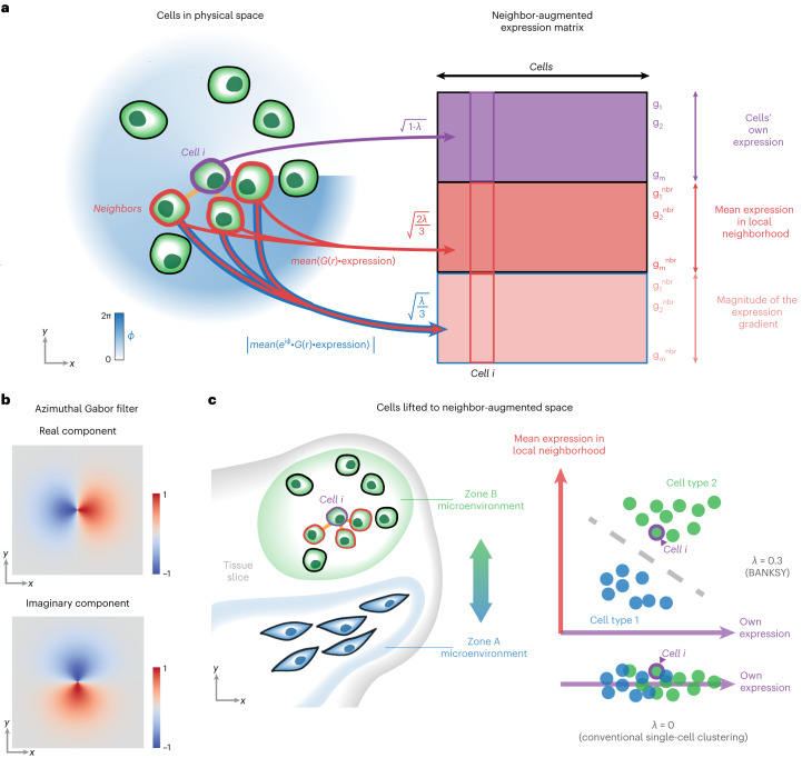
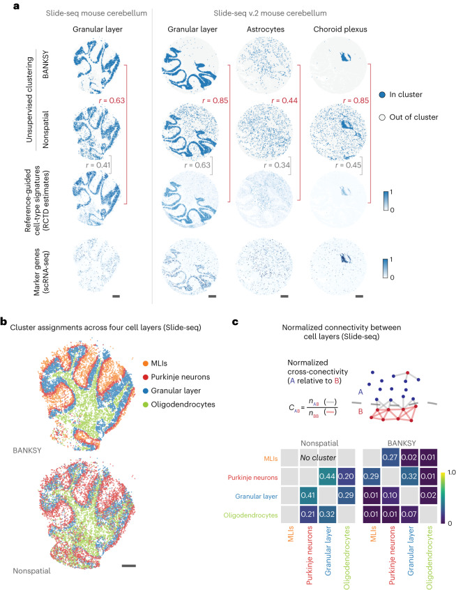
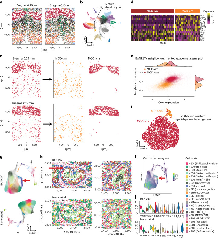
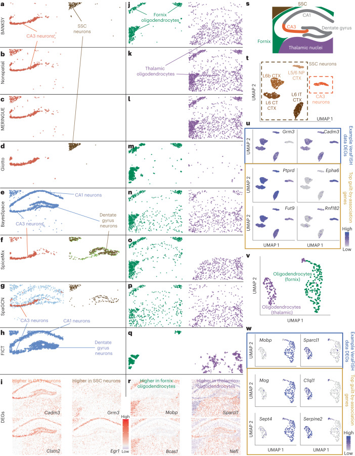
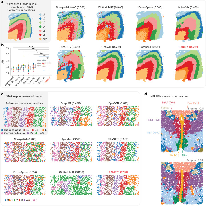
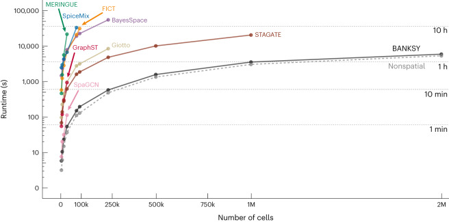
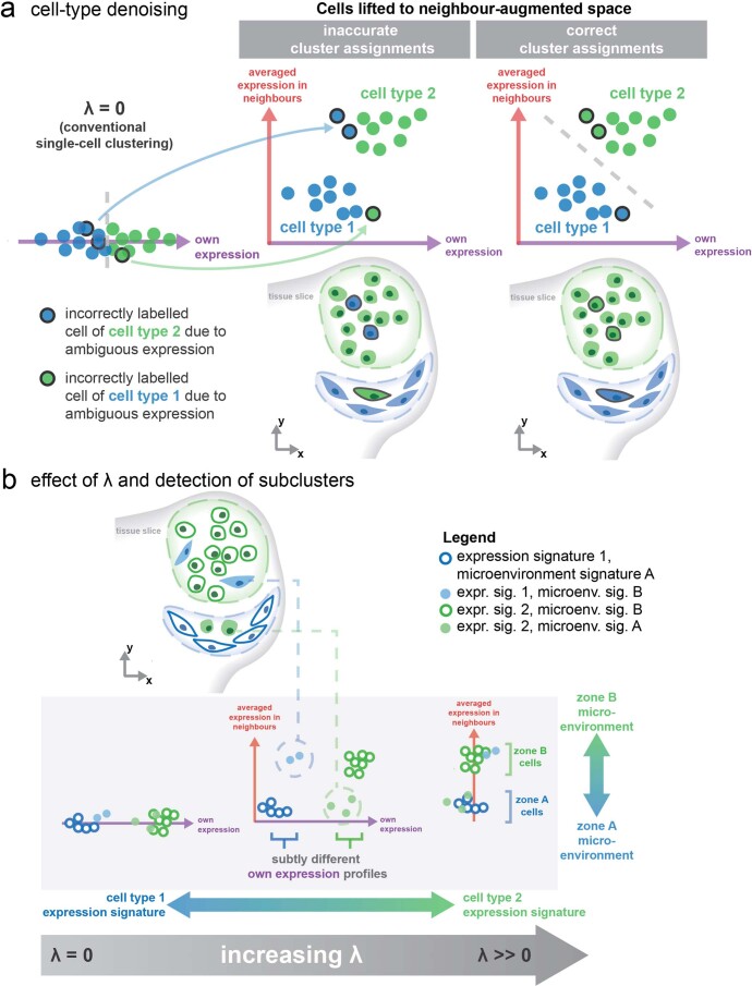
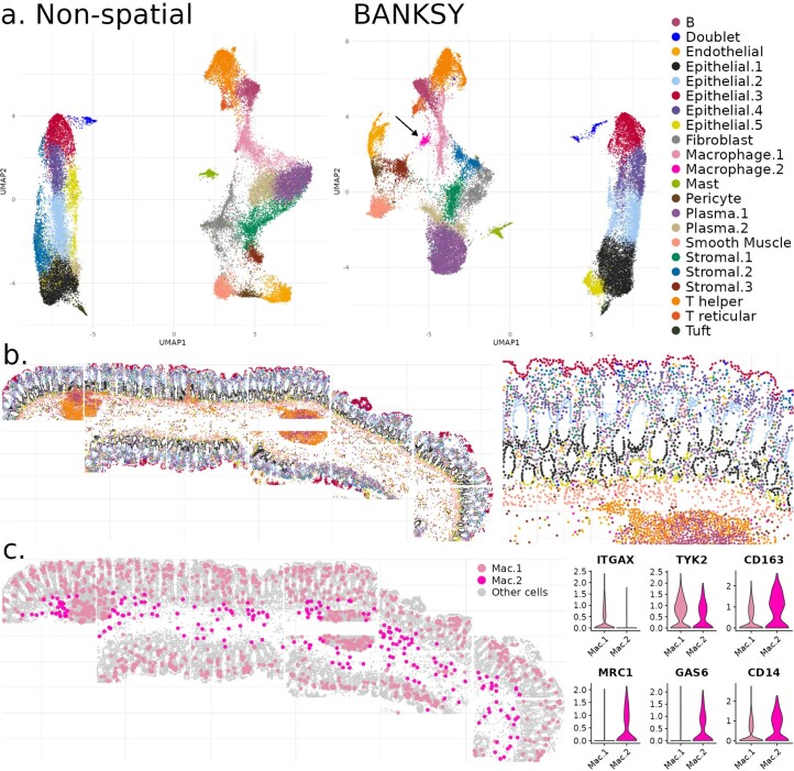
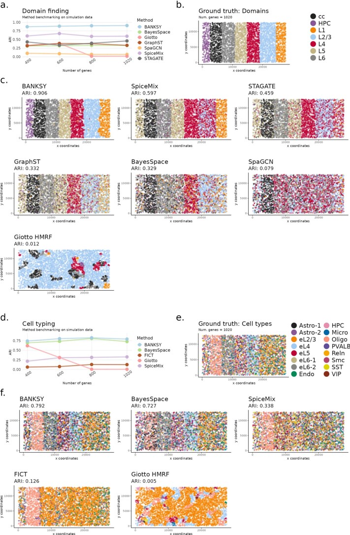
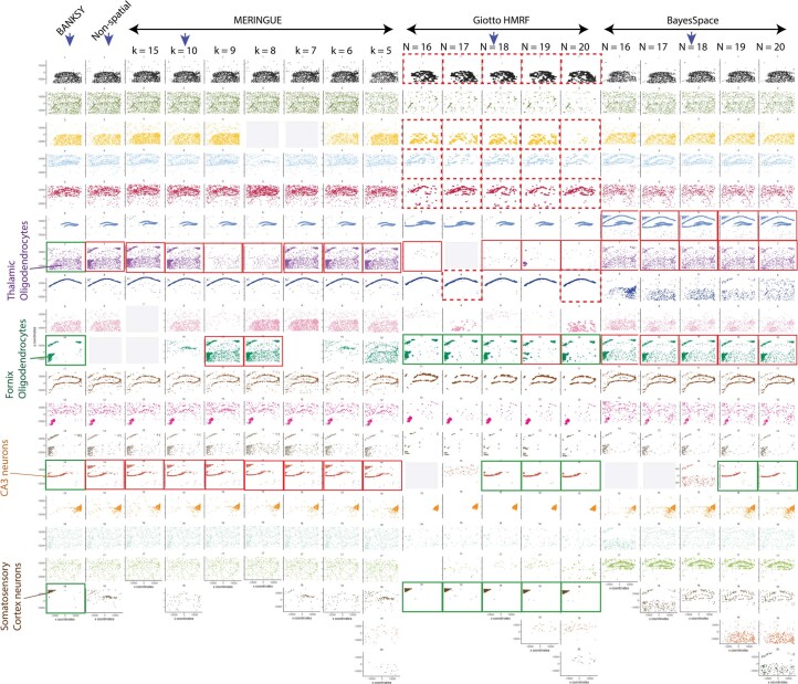
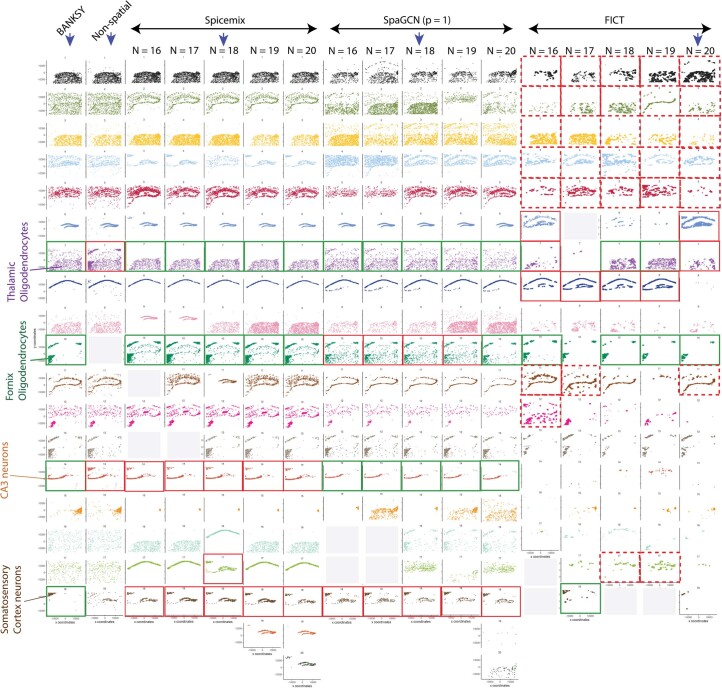
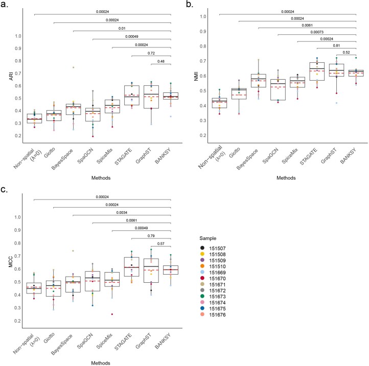
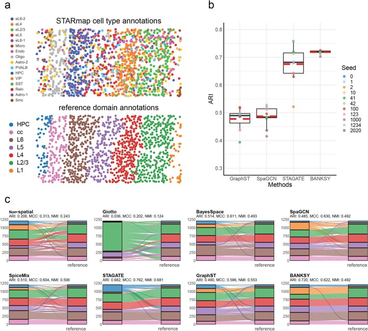
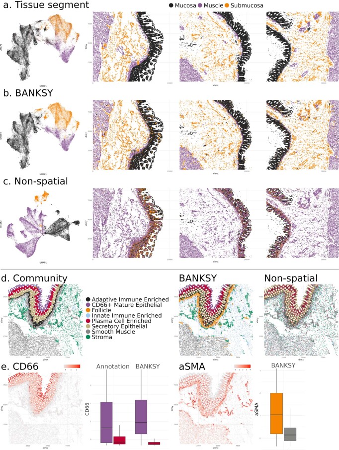
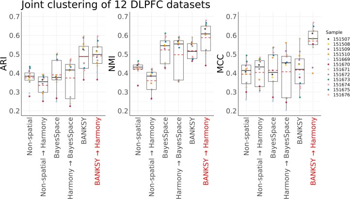
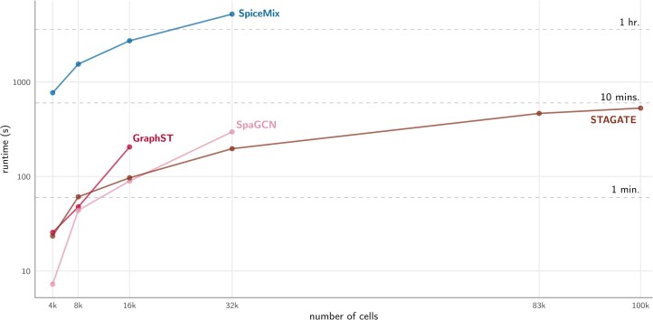
Verification
Claims the paper makes
The claims and statistics of this paper haven’t been checked yet.
Run the check — free, no account needed. It reads the open-access text and checks the sources it cites.
Claims other papers make about this one
Each is checked against this paper’s own text: does it say what the citing paper says it does?
The cited source says what the claim attributes to it.
In the citing paper
“Using BANKSY50-derived spatial domains and Harmony39 correction, we identified 18 reproducible niches shared across 20 samples (Figures S5A–S5C; STAR Methods).”
From Cellular senescence in human liver under normal aging and cancer (2026) · cites this paper as [50]
Self-check
Percentages, sums and reported differences re-computed from the paper’s own numbers.
The self-check needs the paper’s full text.
Citations
Cites
SciPy 1.0: fundamental algorithms for scientific computing in Python
Virtanen, P., Gommers, R., Oliphant, T. E., Haberland, M., Reddy, T., Cournapeau, D., Burovski, E., Peterson, P., Weckesser, W., Bright, J., et al. (2020) · Nature Methods · doi:10.1038/s41592-019-0686-2 · Cited by 38,430
Efficient Estimation of Word Representations in Vector Space
Mikolov, T., Chen, K., Corrado, G., & Dean, J. (2013) · arXiv · doi:10.48550/arxiv.1301.3781 · Cited by 26,568
Self-citationFast unfolding of communities in large networks
Blondel, V. D., Guillaume, J.-L., Lambiotte, R., & Lefebvre, E. (2008) · Journal of Statistical Mechanics: Theory and Experiment · doi:10.1088/1742-5468/2008/10/p10008 · Cited by 21,424
Integrated analysis of multimodal single-cell data
Hao, Y., Hao, S., Andersen-Nissen, E., Mauck, W. M., Zheng, S., Butler, A., Lee, M. J., Wilk, A. J., Darby, C., Zagar, M., et al. (2020) · doi:10.1101/2020.10.12.335331 · Cited by 15,508
Comprehensive Integration of Single-Cell Data
Stuart, T., Butler, A., Hoffman, P., Hafemeister, C., Papalexi, E., Mauck, W. M., Hao, Y., Stoeckius, M., Smibert, P., & Satija, R. (2019) · Cell · doi:10.1016/j.cell.2019.05.031 · Cited by 15,453
The Hungarian method for the assignment problem
Kuhn, H. W. (1955) · Naval Research Logistics Quarterly · doi:10.1002/nav.3800020109 · Cited by 13,120
Fast, sensitive and accurate integration of single-cell data with Harmony
Korsunsky, I., Millard, N., Fan, J., Slowikowski, K., Zhang, F., Wei, K., Baglaenko, Y., Brenner, M., Loh, P.-R., & Raychaudhuri, S. (2019) · Nature Methods · doi:10.1038/s41592-019-0619-0 · Cited by 10,488
SciPy 1.0: fundamental algorithms for scientific computing in Python
Virtanen, P., Gommers, R., Oliphant, T. E., Haberland, M., Reddy, T., Cournapeau, D., Burovski, E., Peterson, P., Weckesser, W., Bright, J., et al. (2019) · Apollo - University of Cambridge Repository · doi:10.17863/cam.64134 · Cited by 10,460
SCANPY: large-scale single-cell gene expression data analysis
Wolf, F. A., Angerer, P., & Theis, F. J. (2018) · Genome Biology · doi:10.1186/s13059-017-1382-0 · Cited by 8,881
Macrophage activation and polarization: nomenclature and experimental guidelines
Murray, P. J., Allen, J. E., Biswas, S. K., Fisher, E. A., Gilroy, D. W., Goerdt, S., Gordon, S., Hamilton, J. A., Ivashkiv, L. B., Lawrence, T., et al. (2014) · Immunity · doi:10.1016/j.immuni.2014.06.008 · Cited by 6,337
Research works printed but not linked: 3
- Huuki-Myers, L. et al. Integrated single cell and unsupervised spatial transcriptomic analysis defines molecular anatomy of the human dorsolateral prefrontal cortex. Preprint at bioRxiv https://doi.org/10.1101/2023.02.15.528722 (2023). · DOI
- Gabor, D. Theory of communication. J. Inst. Electrical Engineering 93, 429–441 (1946).
- Csardi, G. & Nepusz, T. The igraph software package for complex network research. Int. J. Complex Syst. 1695, 1–9 (2006).
Cited by
Sorted by citations
Items 201–284 of 284
Hu, Y., Xie, M., Li, Y., Rao, M., Shen, W., Luo, C., Qin, H., Baek, J., & Zhou, X. M. (2024) · Figshare · doi:10.6084/m9.figshare.26531073
Stassen, S. V., Kobashi, M., Lam, E. Y. M., Huang, Y., Ho, J. W. K., & Tsia, K. K. (2024) · Figshare · doi:10.6084/m9.figshare.26777827
Microenvironment-aware spatial modeling for accurate inference of cell identity
Liu, Q., Wang, Y., Hsu, C., Wanjalla, C. N., Lau, K. S., & Shyr, Y. (2025) · Nucleic Acids Research · doi:10.1093/nar/gkaf1477
Li, J., Yan, J., Liao, Y., Liao, W., Liu, Y., & Cai, H. (2026) · IEEE Journal of Biomedical and Health Informatics · doi:10.1109/jbhi.2025.3644379
Wang, H., Zhang, W., Liu, Z., & Ma, X. (2026) · PLoS Computational Biology · doi:10.1371/journal.pcbi.1013867 · Cited by 1
Xiong, Y., Zito, A., Liang, H., Biouss, G., Yang, J., Balsamo, F., Yeganeh, M., Lee, C., Lee, D., Wang, C.-Y., et al. (2026) · Cellular and Molecular Gastroenterology and Hepatology · doi:10.1016/j.jcmgh.2026.101730 · Cited by 3
Piao, H., Chen, D., Feng, T., Wang, Y., Pei, S., & Wang, Q. (2026) · Research Square · doi:10.21203/rs.3.rs-8197716/v1
Köhler, D., Kleinenkuhnen, N., Rastegar, K., Baar, T., Nikopoulou, C., Kondylis, V., Milchevskaya, V., Schmid, M., Tessarz, P., & Tresch, A. (2026) · Bioinformatics · doi:10.1093/bioinformatics/btag052
CEMUSA: a graph-based integrative metric for evaluating clusters in spatial transcriptomics
Hu, J., Du, Y., Hou, S., Ding, Y., Li, J., Wu, H., & Sun, X. (2026) · Bioinformatics · doi:10.1093/bioinformatics/btag056 · Cited by 1
JGR-NMF: joint graph-regularized non-negative matrix factorization for spatial domain identification
Liang, J., Huang, J., Xi, C., Wang, Y., & Li, J. (2026) · PeerJ · doi:10.7717/peerj.20585 · Cited by 1
Reconstructing multi-scale tissue spatial architecture from single-cell RNA-seq with REMAPPreprint
Jiang, S., Coleman, K., Chen, Z., Jin, K., Liu, Y., Lee, D. H., Hwang, T. H., Xiao, R., Jin, J., Walsh, C. A., et al. (2026) · bioRxiv (Cold Spring Harbor Laboratory) · doi:10.64898/2026.02.21.707167 · Cited by 1
Benchmarking niche identification via domain segmentation for spatial transcriptomics dataPreprint
Wang, Y., Chen, Y., Yang, L., Wang, C., Cai, J., & Xin, H. (2026) · bioRxiv (Cold Spring Harbor Laboratory) · doi:10.64898/2026.02.27.708202 · Cited by 1
Spatial transcriptomic map of the mouse urinary bladder
Matković, N., Gelemanović, A., Popović, K., Vilović, K., Oneto, C., Lazarević, D., Marinovic‐Terzić, I., Novak, I., Korać-Prlić, J., Roje, B. M., et al. (2026) · Scientific Reports · doi:10.1038/s41598-026-42931-z
Composition‐Aware Cross‐Sectional Integration for Spatial Transcriptomics
Dong, Q., Huang, Z., Wang, X., Feng, Z., Liu, W., & Huang, B. (2026) · Advanced Intelligent Discovery · doi:10.1002/aidi.202500226
Liu, K., Liao, S., Li, X., Song, L., Poo, M.-M., Zhao, J., Zhou, W., Cai, R., Wang, M., Ma, X., et al. (2026) · Cell Research · doi:10.1038/s41422-026-01246-4
Multi-omic analyses to characterize retinoblastoma heterogeneity and clonal evolution
Hua, C. (2024) · theses.fr (ABES) · doi:10.70675/317c0f7azf042z488eza0ddz1ec00ba2ac96
Liang, Z., Zhong, B., Jiao, M., Wang, Y., & Liu, S. (2026) · Nature Communications · doi:10.1038/s41467-026-71759-4
Concordia: Spatial Domain Detection via Augmented Graphs for Population-Level Spatial ProteomicsPreprint
Liu, S., Hsu, L., & Sun, W. (2026) · bioRxiv (Cold Spring Harbor Laboratory) · doi:10.64898/2026.04.19.719422
An, S., Keller, M. S., Gehlenborg, N., & Hemberg, M. (2026) · bioRxiv (Cold Spring Harbor Laboratory) · doi:10.64898/2026.04.22.720136 · Cited by 1
Kojima, Y., Tanaka, Y., Hirose, H., Chiwaki, F., Nishimura, K., Hayashi, S., Itahashi, K., Ishikawa, M., Shimamura, T., & Mano, H. (2026) · bioRxiv (Cold Spring Harbor Laboratory) · doi:10.64898/2026.04.21.719876
Magoulopoulou, A., Chatzinikolaou, M. P., Metousis, A., Hu, T., Yu, H., Zerdes, I., Wang, K., Foukakis, T., Long, M., Leandersson, K., et al. (2026) · EBioMedicine · doi:10.1016/j.ebiom.2026.106264
Spatiotemporal single-cell atlas of suture stem cell dynamics in craniosynostosis
Chen, X. W., Lai, C., He, T., Chen, Z., & Jin, X. (2026) · Stem Cell Research & Therapy · doi:10.1186/s13287-026-04987-6
InterScale reveals multi-scale cellular interaction programs in spatial transcriptomicsPreprint
Drummer, F., Jiménez, S., Marco, F. D., Schaar, A. C., Pentimalli, T. M., Beckmann, J., Rajewsky, N., & Theis, F. J. (2026) · bioRxiv (Cold Spring Harbor Laboratory) · doi:10.64898/2026.05.07.723456
Shree, A., Aditya, V., Kumar, T., & Zafar, H. (2026) · bioRxiv (Cold Spring Harbor Laboratory) · doi:10.64898/2026.05.11.724248
Su, J. E., Chen, S., Mankala, S., Zhou, W., Liu, T., Zhao, Y., & Wang, X. (2025) · International Conference on Computational Biology and Bioinformatics (ICCBB) · doi:10.1145/3789938.3789958
Bian, B., Cao, Y., & Yang, J. Y. H. (2026) · Briefings in Bioinformatics · doi:10.1093/bib/bbag176
Deciphering interaction syntax via decoupling intrinsic lineages and niche pressurePreprint
Guo, Q., Zhong, W., Zeng, Z. Q., Nie, Q. H., Zhou, P., & Zhang, L. (2026) · bioRxiv (Cold Spring Harbor Laboratory) · doi:10.64898/2026.05.18.725889
Mao, Y., Quan, L., Chen, X., Wang, S. Q., Zhang, G., Li, S., Jiang, Y., Nie, L., Wu, T., Meng, L., et al. (2026) · Briefings in Bioinformatics · doi:10.1093/bib/bbag248
Ma, H., 黄深思, Wang, H., Zhao, J., & Xia, J. (2026) · IEEE Transactions on Computational Biology and Bioinformatics · doi:10.1109/tcbbio.2026.3697726
Ni, R., Dong, H., Han, R.-D., Ren, X.-C., Qu, Y., Wang, L., Chen, S.-S., & Zhang, Y.-C. (2026) · World Journal of Gastrointestinal Oncology · doi:10.4251/wjgo.121446
Li, Z., Luo, M., Zhu, M., & Bai, Y. (2026) · Genes · doi:10.3390/genes17060616
Generalisable tissue-wide molecular reconstruction from histologyPreprint
Zhang, A., Yu, L., Bian, B., Cao, Y., Ye, S., Han, E., Robertson, H., Dong, Y., Mao, Y., Liu, B., et al. (2026) · bioRxiv (Cold Spring Harbor Laboratory) · doi:10.64898/2026.06.09.731252
SECTOR: structural entropy-based learning of spatiotemporal organisation in spatial transcriptomics
Huang, L., Zhang, J., Gong, W., Zeng, G., Peng, H., & Chen, D. (2026) · Bioinformatics · doi:10.1093/bioinformatics/btag367
Multicellular ecosystems: Linking cellular diversity to tissue function and disease
Shi, Q., Tang, F., Chen, Y., & Zhang, Z. (2026) · Trends in Cell Biology · doi:10.1016/j.tcb.2026.06.005 · Cited by 1
Fault-tolerant 3D reconstruction from 2D spatial proteomics sectionsPreprint
Zhang, Z., Tan, Y., Snyder, M. P., Nolan, G. P., & Ma, Z. (2026) · bioRxiv (Cold Spring Harbor Laboratory) · doi:10.64898/2026.06.23.733649
An integrated skin cell atlas decodes the pilosebaceous unit
Düz, T., Törőcsik, D., Momnougui, S. M. E., Oubounyt, M., Al, B., Gallinat, S., Baumbach, J., & Holzscheck, N. (2026) · Journal of Investigative Dermatology · doi:10.1016/j.jid.2026.06.1282 · Cited by 1
Mitsuhashi, H., Rao, H. R., Amadei, S. S., Chawla, A., Davoli, M. A., Mechawar, N., Turecki, G., & Nagy, C. (2026) · bioRxiv (Cold Spring Harbor Laboratory) · doi:10.64898/2026.07.02.735636
Accessible spatial host–microbe profiling in tumour tissuesPreprint
Wan, Y. K., Ng, A., Tham, J. Y., Li, B., Lim, M., Tan, I. B. H., Prabhakar, S., Nagarajan, N., Yeo, G. H. T., & Chia, M. (2026) · bioRxiv (Cold Spring Harbor Laboratory) · doi:10.64898/2026.07.02.735997
Self-citationDai, R., Wang, Z., Zhang, Z., Lei, L., Wang, M., Li, Z., Liu, X., & Guo, Q. (2026) · Functional & Integrative Genomics · doi:10.1007/s10142-026-01960-7
wang, H., Yang, X., Wang, S., Yang, Z., Yang, X., Yang, Y., Li, Z., Ren, Y., Zhang, Q., Zhao, B., et al. (2026) · iMeta · doi:10.1002/imt2.70146
Structural-information guided fusion for spatial domain identification from spatial transcriptomics
Zhang, M., Gao, P., Chen, C., Ma, X. Y., Chen, X., & Feng, S. (2026) · Bioinformatics · doi:10.1093/bioinformatics/btag508
Li, X., Jiang, X. Y., Dong, Q., Wu, J., Li, Y., Zhang, Y., & Zhong, L. (2026) · medRxiv · doi:10.64898/2026.06.30.26356926
Ependymomas are cancers of the pre-neural crest/roof plate lineagePreprint
Balin, P., Kumar, S. A., Galton, R., Delaidelli, A., Orisme, W., Haldipur, P., Mankahla, N., Saadeldin, A. M., von Krosigk, N., Vladoiu, M. C., et al. (2026) · bioRxiv (Cold Spring Harbor Laboratory) · doi:10.64898/2026.07.13.736818
Self-citationWu, C., Luo, X., Zhao, Y., Chen, Y., & Zuo, N. (2026) · Briefings in Bioinformatics · doi:10.1093/bib/bbag362
SEMA: A Framework of Spatial-Aware Enrichment for Multi-pathway AnalysisPreprint
Fan, X. (2026) · Research Square · doi:10.21203/rs.3.rs-10387597/v1
Yu, T., Zhang, M., Zhou, J., & Lu, X. (2026) · Expert Systems with Applications · doi:10.1016/j.eswa.2026.133725
Mao, Q., Ahmadi, A., de Vries, S. I., Heezen, L. G. M., Vacca, O., Doisy, M., Aartsma-Rus, A. M., van Putten, M., Goyenvalle, A., Mahfouz, A. E., et al. (2026) · iScience · doi:10.1016/j.isci.2026.116906
Birk, S., Merchant, A., Vahidi, A., Theis, F. J., & Lotfollahi, M. (2026) · bioRxiv (Cold Spring Harbor Laboratory) · doi:10.64898/2026.08.07.743490
Deep-learning-driven tumor microenvironment profiling improves immunotherapy response predictionPreprint
Wang, R., Benard, B. A., Ilerten, I., Zdravkovic, S., Al-Humadi, R., Nasr, S., Howitt, B., & Gentles, A. J. (2026) · bioRxiv (Cold Spring Harbor Laboratory) · doi:10.64898/2026.10.06.757143
Totty, M. S., Bach, S. V., Valentine, M. R., Tippani, M., Maguire, S. E., Rosario, I. D., Miller, R. A., Kleinman, J. E., Maynard, K. R., Page, S. C., et al. (2026) · bioRxiv (Cold Spring Harbor Laboratory) · doi:10.64898/2026.08.22.746381
Paired-surface spatial mechanomics links tissue stiffness maps to spatial transcriptomicsPreprint
Ong, H. T., Lou, Y., Turley, J., Hengst, R. M., Ramli, M. F. H., Shen, X., Marlena, J., Zhu, J., Li, R., Chan, C. J., et al. (2026) · bioRxiv (Cold Spring Harbor Laboratory) · doi:10.64898/2026.08.29.748050
Zahedi, R., Argha, A., Farbehi, N., Bakhshayeshi, I., Porntaveetus, T., Ye, Y., Lovell, N. H., & Alinejad‐Rokny, H. (2026) · Advanced Science · doi:10.1002/advs.77003 · Cited by 1
Webber, E., Porter, K., Li, L. Z., Aksu, M., & Gasier, H. G. (2026) · Experimental Neurology · doi:10.1016/j.expneurol.2026.116004
Xu, M., Dong, Z., & Xia, B. (2026) · Briefings in Bioinformatics · doi:10.1093/bib/bbag480
Chopp, L. B., Xing, X., Wasikowski, R., Fox, J. P., Kirma, J., Kahlenberg, J. M., Tsoi, L. C., Chan, M. P., & Gudjonsson, J. E. (2026) · Journal of Investigative Dermatology · doi:10.1016/j.jid.2026.08.011
Hai, C., Hou, Y., Yu, S., Pan, X., Nicolas, G. M., Li, P., Gungor, C., Yuan, T., Wang, Z., Wang, Z., et al. (2026) · Gut · doi:10.1136/gutjnl-2026-338471
Li, J., Garg, V., Martiartu, A., Tanzillo, A. F., Zhang, Y., & Petros, T. J. (2026) · bioRxiv (Cold Spring Harbor Laboratory) · doi:10.64898/2026.09.08.749487
Sun, P., Wang, J., Wang, Y., Zhang, Y., Tang, Y., Yang, J., & Wang, Z. (2026) · Research Square · doi:10.21203/rs.3.rs-10804793/v1
Tang, B., Mao, M., Li, J., & Zhou, F. (2026) · Pattern Recognition · doi:10.1016/j.patcog.2026.114923
Huang, Y., Zhang, J., Lou, J., Bian, B., Zhang, M., Gou, T., Jiang, T., & Zhang, G. (2026) · Cells · doi:10.3390/cells15181676
Structure-Aware Multi-Modal Fusion for Interpretable Niche Prediction in Spatial Omics
Jiang, P., Shi, B., Qin, Y., Li, Y., Wang, Q., Sataer, Y., & Tao, X. (2026) · International Symposium on Communications and Information Technologies · doi:10.1109/iscit70453.2026.11695369
Xia, Y., Ji, X., Liu, H., Guo, F., Feng, X., He, L., Cui, H., Xu, S., Su, R., Wei, L., et al. (2026) · Lecture notes in computer science · doi:10.1007/978-3-032-38069-2_34
Shi, H., Zhang, X., Shouliang, C., Xu, B., Wang, H., Cui, J., Yang, Z., Chen, S., Zhou, Z., Zhang, S., et al. (2026) · Science Advances · doi:10.1126/sciadv.aeg7722
The tumor microenvironment landscape in lung adenocarcinoma with spatial transcriptomic mappingPreprint
Nie¹, J., Song¹, W., Yang, B., Li¹, X., Li¹, W., Duan, P., Lv, X., & Hou, S. (2026) · Research Square · doi:10.21203/rs.3.rs-10946821/v1
A meta-interaction basis for cell-cell communication in tissuesPreprint
Tang, J., Liang, S., Alam, S., Cheng, W., Zhang, Y., & Ma, J. (2026) · bioRxiv (Cold Spring Harbor Laboratory) · doi:10.64898/2026.09.21.753369
Trustworthy super-resolution reconstruction across spatial omics modalitiesPreprint
Li, M.-H., Wang, X.-T., Xu, S.-S.-G.-H.-J.-B.-S.-W.-Z.-C.-X.-L., Yin, Y.-X., Chen, D., Guo, X.-C., & Song, D.-Y. (2026) · bioRxiv · doi:10.64898/2026.09.25.754471
Spatial evolution of a cachexia-promoting microenvironment in pancreatic cancer
Hu, Y., Lv, G., Yuan, H., Zhou, Z., Zhang, S., Ye, Y., Chen, Q., Cai, Y., Yang, J., Zhang, Y., et al. (2026) · Cell · doi:10.1016/j.cell.2026.09.012 · Cited by 1
Edula, C. S. R., Sun, Y., & Zhang, X. (2026) · Journal of Computational Biology · doi:10.1177/15578666261491611
Spatial transcriptomics profiling across tissue boundaries in the developing mouse brain
Hammer, V., & Ossowski, S. (2026) · iScience · doi:10.1016/j.isci.2026.117765
Zhu, L., Dong, H., Zhang, Y., Zhang, Y., Xinyi, 黄. H., & Wang, H. (2026) · Frontiers in Physiology · doi:10.3389/fphys.2026.1967219
VINTER: a generative vision–language model for annotating and interrogating spatial tissuesPreprint
JinYu, W., Xu, W., Zhuang, Y., Zhang, Y., Loza, M., Yang, Y., & Nakai, K. (2026) · bioRxiv (Cold Spring Harbor Laboratory) · doi:10.64898/2026.10.01.752251
Zhong, Z., Zhu, X., Guo, J., Liao, S., & Chen, A. (2026) · Briefings in Bioinformatics · doi:10.1093/bib/bbag512
Micu, A., Matei, A., Li, Y., Pecher, A., Filla, T., Bruch, P., Dietrich, S., Henes, J. C., Zweck, E., Eckstein, M., et al. (2026) · bioRxiv (Cold Spring Harbor Laboratory) · doi:10.64898/2026.10.06.756898
Scalable localization of clustering instability for spatial transcriptomicsPreprint
Wu, W., Nguyen, J. T., & Molloy, E. K. (2026) · bioRxiv (Cold Spring Harbor Laboratory) · doi:10.64898/2026.10.08.738042
li, Z., & Yang, J. (2026) · bioRxiv (Cold Spring Harbor Laboratory) · doi:10.64898/2026.10.08.757757
Leon, J., Yoshinaga, S., Koya, I., Palafox, G., Ando, Y., Kubo, K., Moody, J., Takao, M., Carninci, P., Shin, J. W., et al. (2026) · bioRxiv (Cold Spring Harbor Laboratory) · doi:10.64898/2026.10.07.757387
Huo, M., Xue, Z., Sheng, Y., & Li, S. (2026) · Frontiers in Materials · doi:10.3389/fmats.2026.1969087
SpatialZoomer: multi-scale feature analysis of spatial transcriptomics
Li, X., Fan, Y., Han, Y., Guo, W., Huang, J., Yan, N., Chen, Z., Wu, Y., Miao, Y., Hou, L., et al. (2026) · Nature Biomedical Engineering · doi:10.1038/s41551-026-01800-w
ALBIS: simulation of multi-resolution and multi-dimensional spatial transcriptomics dataPreprint
Matthias, J., Yao, J., & Hicks, S. C. (2026) · bioRxiv (Cold Spring Harbor Laboratory) · doi:10.64898/2026.10.06.757026
Wyler, E., Albertini, S., Friedel, C. C., Manukyan, A., Winterfeldt, A., Bracker, N., Huang, J., Krasemann, S., Plumbom, I., Altmüller, J., et al. (2026) · Science Advances · doi:10.1126/sciadv.aef5563
Donor-Resolved Analysis of HES1-Associated Fibroblast States in Systemic Sclerosis
shenyi, F., Huang, L., & Wang, M. (2026) · Biomedicines · doi:10.3390/biomedicines14102360
Artificial intelligence in spatial transcriptomics: a review of methods, datasets, and directions
Sharma, N., Şen, R., & Erdem, C. (2026) · Briefings in Bioinformatics · doi:10.1093/bib/bbag569
Identification and characterization of neoplastic cells in keratin-positive giant cell–rich tumors
van der Linde, R. M., Chrisinger, J. S. A., Demicco, E. G., Dehner, C. A., Charville, G. W., Bruijn, I. H. B., Varma, S., Zhu, C., Matusiak, M., Bovée, J. V. M. G., et al. (2026) · Proceedings of the National Academy of Sciences · doi:10.1073/pnas.2611959123
Advances in early human embryonic development and organogenesis from spatiotemporal multi-omics
Zhu, H., Yang, X., Wang, X., & Xiao, Z. (2026) · Journal of Translational Genetics and Genomics · doi:10.20517/jtgg.2026.26
Metadata
- Authors
- Singhal, V., Chou, N., Lee, J., Yue, Y., Liu, J., Chock, W. K., Lin, L., Chang, Y.-C., Teo, E. M. L., Aow, J., Lee, H. K., Chen, K. H., & Prabhakar, S.
- Affiliations
- Agency for Science, Technology and Research (SG)
- National University of Singapore (SG)
- Corresponding author
- Chen, Kok Hao
- Prabhakar, Shyam
- ORCID
- Venue
- Nature Genetics
- Published
- 2024-02-27
- Volume
- 56
- Issue
- 3
- Pages
- 431-441
- ISSN
- 1061-4036 (ISSN-L)
- 1546-1718
- PMC
- PMC10937399
- OpenAlex
- W4392198237
- Cited by
- 282
- References
- 77
- Citations by year
- 2026: 124 · 2025: 103 · 2024: 47
- FWCI
- 37.44
- Type
- journal article
- Language
- en
- Open access
- hybrid
- doi.org
- Locations
- Nature Genetics (publishedVersion, cc-by)
- bioRxiv (Cold Spring Harbor Laboratory) (acceptedVersion, cc-by-nc-nd)
- PubMed Central (publishedVersion, cc-by)
- PubMed (publishedVersion)
- DR-NTU (Nanyang Technological University) (submittedVersion, cc-by)
- Funders
- MOH | National Medical Research Council (OFIRG21jun-0090, OF-YIRG18nov-0014, OFIRG-000618-00)
- Agency for Science, Technology and Research (#H18/01/a0/020, 202D800010, H18/01/a0/020, I1801E0029)
- National Research Foundation Singapore (NRF-CRP25-2020-0001)
- Topics
- Life Sciences › Biochemistry, Genetics and Molecular Biology › Molecular Biology › Single-cell and spatial transcriptomics
- Life Sciences › Biochemistry, Genetics and Molecular Biology › Biophysics › Cell Image Analysis Techniques
- Life Sciences › Biochemistry, Genetics and Molecular Biology › Molecular Biology › Gene expression and cancer classification
- Keywords
- spatial omics, cell typing, spatial clustering, mouse brain, batch effect correction, scalable data analysis
- MeSH terms
- Data Analysis, Algorithms, Animals, RNA, Benchmarking, Gene Expression Profiling, Mice, Transcriptome
About these checks
Registry, retraction, Cites and statistics results are computed, not judged, with one exception: a printed reference that no index lists is read once by a model before it counts as a citation error. Claims are extracted by a model and kept only when their quote appears verbatim in the text; each cited source is then checked, with a model’s help, for whether it says what the claim relies on. Those verdicts can be wrong — read the claim’s quote and the cited source before relying on one.
Statistics and arithmetic are recomputed, not judged.
Confidence bands are shown only for fields calibrated on our annotated test set. None is calibrated yet, so no band is shown.
What counts as a claim ›How we measure confidence ›How we check this ›
Are you an author, or do you see a problem with this page? Request a review
