

The DOI matches its Crossref record; 122 of the 122 references it cites were found in a registry or an index; 74 of the 92 sources its claims cite were checked for support.
Predicting RNA-seq coverage from DNA sequence as a unifying model of gene regulation
Open accessPublished version of a preprint
Abstract
Sequence-based machine-learning models trained on genomics data improve genetic variant interpretation by providing functional predictions describing their impact on the cis-regulatory code. However, current tools do not predict RNA-seq expression profiles because of modeling challenges. Here, we introduce Borzoi, a model that learns to predict cell-type-specific and tissue-specific RNA-seq coverage from DNA sequence. Using statistics derived from Borzoi's predicted coverage, we isolate and accurately score DNA variant effects across multiple layers of regulation, including transcription, splicing and polyadenylation. Evaluated on quantitative trait loci, Borzoi is competitive with and often outperforms state-of-the-art models trained on individual regulatory functions. By applying attribution methods to the derived statistics, we extract cis-regulatory motifs driving RNA expression and post-transcriptional regulation in normal tissues. The wide availability of RNA-seq data across species, conditions and assays profiling specific aspects of regulation emphasizes the potential of this approach to decipher the mapping from DNA sequence to regulatory function.
Overview
AI snapshot
Written from the paper’s full text.
TL;DR
Borzoi is a sequence-based neural network that predicts cell-type- and tissue-specific RNA-seq coverage directly from DNA sequence, enabling variant-effect scoring across transcription, splicing and polyadenylation. It performs competitively with or better than state-of-the-art models on several QTL and regulatory-variant tasks while also recovering known cis-regulatory motifs.
Key findings
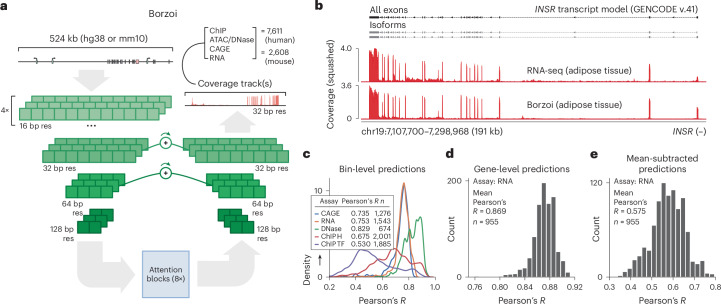
- Borzoi predicts RNA-seq coverage with mean Pearson’s R = 0.74 per model replicate and 0.75 for the ensemble across human samples; gene-level Pearson’s R = 0.87, and residual across-track Pearson’s R = 0.58.
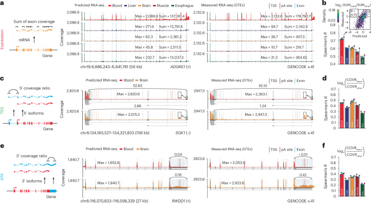
- In five GTEx tissues, predicted versus measured tissue-specific expression fold-change correlations ranged from Spearman’s R = 0.52 to 0.75; TSS usage correlations were R = 0.85 pooled and R = 0.29–0.50 tissue-specific; APA correlations were R = 0.81 pooled and R = 0.23–0.41 tissue-specific.
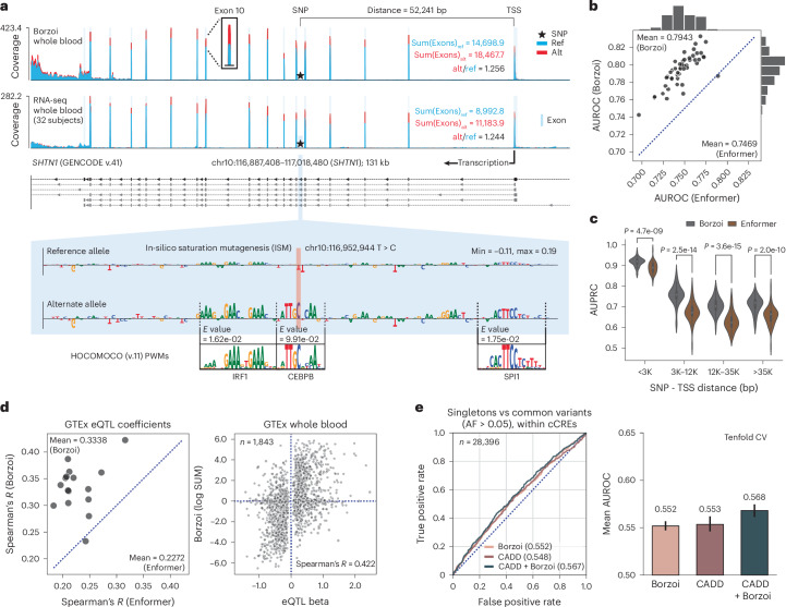
- Borzoi discriminated fine-mapped GTEx eQTLs from matched negatives with mean AUROC = 0.794 versus Enformer’s 0.747, and predicted eQTL effect sizes with mean Spearman’s R = 0.334 versus Enformer’s 0.227. For paQTLs, Borzoi achieved AUPRC = 0.64–0.74 and outperformed APARENT2; for sQTLs, Pangolin had a slight overall advantage (dAUPRC = 0.01) but Borzoi was better near splice junctions (dAUPRC = 0.02).
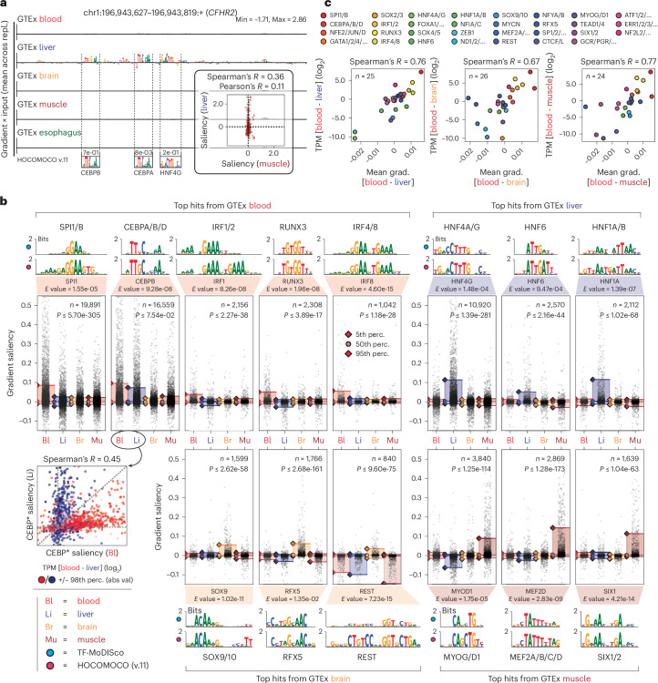
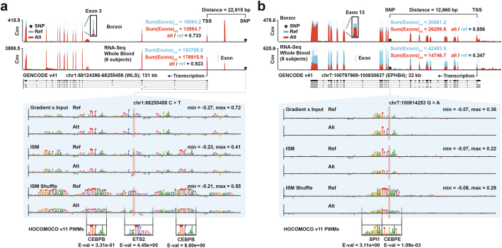
- Motif discovery recovered known regulators such as SPI1/B and IRF4/8 in blood, HNF4A/G and HNF1A in liver, SOX9 and REST in brain, and MYOD1 and MEF2D in muscle; TF saliency differences correlated with measured TPM fold changes up to Spearman’s R = 0.77 for blood versus muscle.
Methods
- Borzoi uses an Enformer-like convolution and self-attention core at 128 bp resolution, followed by U-net upsampling to predict coverage in 32 bp bins from 524 kb input sequences.
- Training data included 867 human and 278 mouse ENCODE RNA-seq tracks, GTEx recount3 tracks, and Enformer assays such as CAGE, DNase-seq, ATAC-seq and ChIP–seq; four randomly initialized replicates were trained and ensembled.
- The model was trained with species-specific heads, Poisson and multinomial loss components, and evaluated on held-out genomic partitions for Figs. 1–2; downstream variant analyses used attribution methods, TF-MoDISco/Tomtom motif discovery, and QTL classification/regression benchmarks.
Limitations
- The paper states that Borzoi is far from perfect: most tissue-specific splicing events were not captured well, the model tended to predict average RNA-seq shape, and no sequence elements related to mRNA half-life were found in attributions.
- The paper notes that sequencing bias, such as greater read density at transcript 3′ ends and GC bias, caused false positives when classifying alternatively used splice sites, and that attribution method choice matters, with window-shuffled ISM working better for 3′ UTRs.
- The text also makes evident that Enformer comparisons are imperfect because of different data processing, test sets, bin resolution and CAGE strand splitting; eGene prioritization performed only marginally better than a TSS-distance baseline, and Borzoi and CADD had equal discriminative power for singletons versus common variation (mean AUROC = 0.55).
Model-written summary. Check it against the paper before relying on it.
Integrity signals
Registry
Cites
Statistics
Figures
Verification
Claims the paper makes
69 Own result · 23 No basis given · 21 Own interpretation · 17 Supported · 16 Own method · 9 Partly supported · 5 Supported so far · 4 Couldn’t confirm · 1 Not checked yet · accuracy not yet measured
The cited sources support only part of this claim — read each source’s verdict below.
In the paper
“Thus far, such models have focused on assays in which measured activity is proportional to local sequencing read counts.”
§ Predicting RNA-seq coverage from DNA sequence as a unifying model of gene regulation > Main
What the sources say
- Not checked — no full text of the sourcecites [4] Alipanahi, B., Delong, A., Weirauch, M. T. & Frey, B. J. Predicting the sequence specificities of DNA- and RNA-binding proteins by deep learning. Nat. Biotechnol. 33, 831–838 (2015). source
- Partly supportedcites [5] Zhou, J. & Troyanskaya, O. G. Predicting effects of noncoding variants with deep learning-based sequence model. Nat. Methods 12, 931–934 (2015). sourceExperimental — accuracy not yet measured
The paper describes a sequence-based model trained on TF-binding, DNase I–sensitivity, and histone-mark profiles (Abstract) and uses sequencing reads to assess allelic imbalance (Online Methods, ‘Evaluation of the single-nucleotide sensitivity of chromatin feature prediction’). It does not state that measured activity in these assays is proportional to local read counts, or establish that sequence-based models generally had focused on such assays. Its own training labels are binary peak-overlap labels (Online Methods, ‘Data for training DeepSEA’). (LLM, conf=0.78)
- Partly supportedcites [6] Kelley, D. R., Snoek, J. & Rinn, J. L. Basset: learning the regulatory code of the accessible genome with deep convolutional neural networks. Genome Res. 26, 990–999 (2016). sourceExperimental — accuracy not yet measured
The Results section describes Basset as a sequence-based model of accessibility using DNase-seq data. But Methods (“DNase I hypersensitivity data”; page not provided) says its training labels were binary indicators of significant peaks, not activity values proportional to local sequencing read counts. The paper therefore supports the assay focus but not the claimed read-count relationship. (LLM, conf=0.84)
- Partly supportedcites [7] Avsec, Ž. et al. Base-resolution models of transcription-factor binding reveal soft motif syntax. Nat. Genet. 53, 354–366 (2021). sourceExperimental — accuracy not yet measured
The Introduction (page unavailable) describes existing transcription-factor binding models as predicting binary binding events or continuous binding signals, and the Results describe ChIP-nexus profiles in terms of local read counts. This supports the claim for the transcription-factor binding models discussed, but the paper does not establish that sequence-based models generally had focused on read-count-based assays. (LLM, conf=0.78)
- Supportedcites [8] Kelley, D. R. et al. Sequential regulatory activity prediction across chromosomes with convolutional neural networks. Genome Res. 28, 739–750 (2018). source
The Results (Basenji; page not supplied) describe models of DNase-seq, ChIP-seq, and CAGE assays built from sequencing reads. The Methods (Data preprocessing; page not supplied) state that read-coverage estimates were summed in local genomic bins as the signal to predict, supporting the cited characterization of these assays. (LLM, conf=0.85)
- Partly supportedcites [9] Kelley, D. R. Cross-species regulatory sequence activity prediction. PLoS Comput. Biol. 16, e1008050 (2020). sourceExperimental — accuracy not yet measured
The Materials and methods section (Functional genomics data; page not specified) says the models focused on sequencing assays and describes deriving local signal from aligned reads. But it also says the models used log-fold-change signal tracks for many datasets; those targets are not simply proportional to local read counts. (LLM, conf=0.85)
- Partly supportedcites [10] Chen, K. M., Wong, A. K., Troyanskaya, O. G. & Zhou, J. A sequence-based global map of regulatory activity for deciphering human genetics. Nat. Genet. 54, 940–949 (2022). sourceExperimental — accuracy not yet measured
The Main section says earlier sequence models focused on predicting transcription-factor binding and histone modifications. Results describes Sei’s chromatin-profile targets, but Methods (Deep learning sequence model training; page unavailable) says its training labels are binary peak calls. The paper does not establish that measured activity in these assays is proportional to local sequencing read counts. (LLM, conf=0.78)
plain- Asserted: passes — The authors put it forward as true.
- Checkable: passes — It can be checked against evidence.
- Load-bearing: passes — The paper’s conclusions depend on it.
- Based: passes — The paper gives a reason why it holds.
The cited sources support only part of this claim — read each source’s verdict below.
In the paper
“However, such metrics inevitably struggle to describe complex splicing outcomes, unannotated de novo events or the intricate and sometimes competitive relationship between transcription, splicing and (intronic) polyadenylation24–26.”
§ Predicting RNA-seq coverage from DNA sequence as a unifying model of gene regulation > Main
What the sources say
- Partly supportedcites [24] Hallier, M., Tavitian, A. & Moreau-Gachelin, F. The transcription factor Spi-1/PU.1 binds RNA and interferes with the RNA-binding protein p54nrb. J. Biol. Chem. 271, 11177–11181 (1996). sourceExperimental — accuracy not yet measured
The Results and Discussion report that the transcription factor Spi-1/PU.1 interfered with splicing in an in vitro β-globin assay, offering a limited example of a transcription-associated protein affecting splicing. The paper does not address whether post-transcriptional metrics struggle to describe splicing outcomes, unannotated de novo events, or the relationship with intronic polyadenylation; searches for those terms found no supporting passage. The indexed passages provide no page number for the Results and Discussion. (LLM, conf=0.76)
- Not checked yetcites [25] Oksuz, O. et al. Transcription factors interact with RNA to regulate genes. Mol. Cell 83, 2449–2463.e13 (2023). source
Checked before — its earlier verdict is held back until a new check runs.
- Partly supportedcites [26] Kwon, B. et al. Enhancers regulate 3′ end processing activity to control expression of alternative 3′UTR isoforms. Nat. Commun. 13, 2709 (2022). sourceExperimental — accuracy not yet measured
The Introduction (page unavailable) says it is difficult to disentangle transcript production from processing when assessing expression of single-UTR genes. That supports a narrower version of the claimed complexity, but the paper does not establish that summary metrics inevitably fail to describe complex splicing, unannotated de novo events, or competition with intronic polyadenylation. (LLM, conf=0.76)
plain- Asserted: passes — The authors put it forward as true.
- Checkable: passes — It can be checked against evidence.
- Load-bearing: passes — The paper’s conclusions depend on it.
- Based: passes — The paper gives a reason why it holds.
- Partly supported
The cited sources support only part of this claim — read each source’s verdict below.
In the paper
“Predicted tissue-pooled distal-to-proximal polyadenylation coverage ratios of held-out genes were highly correlated with measurements from GTEx (Spearman’s R = 0.81; Supplementary Fig. 3f) and PolyADB v.3 (refs. 43,44) (Supplementary Fig. 3g).”
§ Predicting RNA-seq coverage from DNA sequence as a unifying model of gene regulation > Results > Inference of tissue-specific expression and isoform usage
What the sources say
- Partly supportedcites [43] Zhang, H., Hu, J., Recce, M. & Tian, B. PolyA_DB: a database for mammalian mRNA polyadenylation. Nucleic Acids Res. 33, D116–D120 (2005). sourceExperimental — accuracy not yet measured
The Results (Data access and visualization; page unavailable) identify polyA_DB as a database of polyadenylation sites, supporting the citation’s identification of the resource. Our copy does not identify the database as PolyADB v.3 or establish that this version supplied the cited measurements. The correlation is presented as a result of the citing study, not a finding attributed to this source. (LLM, conf=0.86)
- Supportedcites [44] Wang, R., Nambiar, R., Zheng, D. & Tian, B. PolyA_DB 3 catalogs cleavage and polyadenylation sites identified by deep sequencing in multiple genomes. Nucleic Acids Res. 46, D315–D319 (2018). source
The citation identifies PolyA_DB version 3 as a source of polyadenylation-site measurements, not as the source of the citing authors’ correlation result. The Summary and Future Directions and Database Content sections describe PolyA_DB 3 as a collection of polyadenylation sites with quantitative usage data, including normalized read counts. (LLM, conf=0.93)
plaincorrelational- Asserted: passes — The authors put it forward as true.
- Checkable: passes — It can be checked against evidence.
- Load-bearing: passes — The paper’s conclusions depend on it.
- Based: passes — The paper gives a reason why it holds.
- Partly supported
Every source the paper cites for this claim was checked and supports it.
In the paper
“Recent work on the Enformer model using self-attention has demonstrated a path toward achieving this goal13.”
§ Predicting RNA-seq coverage from DNA sequence as a unifying model of gene regulation > Main
What the sources say
- Supportedcites [13] Avsec, Ž. et al. Effective gene expression prediction from sequence by integrating long-range interactions. Nat. Methods 18, 1196–1203 (2021). source
The Results section, “Enformer improves gene expression prediction,” says Enformer uses transformer attention layers to integrate information from distal regulatory elements up to 100 kb away. The Methods section, “Model architecture,” likewise says its transformer blocks capture long-range interactions across the sequence. This supports the citing sentence’s characterization of Enformer as a path toward modeling long-range regulatory information. (LLM, conf=0.94)
boostedcorrelational- Asserted: passes — The authors put it forward as true.
- Checkable: passes — It can be checked against evidence.
- Load-bearing: passes — The paper’s conclusions depend on it.
- Based: passes — The paper gives a reason why it holds.
- Supported
The cited sources support only part of this claim — read each source’s verdict below.
In the paper
“Previous models have only attempted to work with RNA-seq after summarizing gene expression in a single statistic.”
§ Predicting RNA-seq coverage from DNA sequence as a unifying model of gene regulation > Main
What the sources say
- Not checked — no full text of the sourcecites [11] Agarwal, V. & Shendure, J. Predicting mRNA abundance directly from genomic sequence using deep convolutional neural networks. Cell Rep. 31, 107663 (2020). source
- Partly supportedcites [12] Zhou, J. et al. Deep learning sequence-based ab initio prediction of variant effects on expression and disease risk. Nat. Genet. 50, 1171–1179 (2018). sourceExperimental — accuracy not yet measured
The Online Methods section on representative transcription start sites says most expression-profiling datasets were quantified at the gene level, including RNA-seq datasets. That supports the idea of summarizing expression, but it does not establish that all previous models worked with RNA-seq only after reducing expression to a single statistic. No page number is available in our copy. (LLM, conf=0.82)
- Partly supportedcites [13] Avsec, Ž. et al. Effective gene expression prediction from sequence by integrating long-range interactions. Nat. Methods 18, 1196–1203 (2021). sourceExperimental — accuracy not yet measured
The Results section (page unavailable) identifies ExPecto as a previous model trained to predict gene-expression levels measured by RNA-seq. It does not say that all previous models used RNA-seq only after reducing expression to a single statistic. The Methods passage about summing CAGE counts describes this paper’s evaluation, not that broader claim about earlier RNA-seq models. (LLM, conf=0.82)
plain- Asserted: passes — The authors put it forward as true.
- Checkable: passes — It can be checked against evidence.
- Load-bearing: passes — The paper’s conclusions depend on it.
- Based: passes — The paper gives a reason why it holds.
The cited sources support only part of this claim — read each source’s verdict below.
In the paper
“Borzoi enables direct characterization of tissue-specific cis-regulatory TF motifs by applying attribution methods to the predicted RNA-seq coverage statistics45–50.”
§ Predicting RNA-seq coverage from DNA sequence as a unifying model of gene regulation > Results > Borzoi identifies regulatory motifs driving RNA expression
What the sources say
- Could not verifycites [45] Talukder, A., Barham, C., Li, X. & Hu, H. Interpretation of deep learning in genomics and epigenomics. Brief. Bioinform. 22, bbaa177 (2021). sourceExperimental — accuracy not yet measured
The Chromatin interactions section describes saliency maps for Basenji, and the Gene expression prediction section discusses RNA-seq as a data source, but neither addresses Borzoi. Searches for Borzoi and for attribution of predicted RNA-seq coverage to tissue-specific TF motifs found no passage supporting the claim in our copy; page numbers were not available. (LLM, conf=0.76)
- Not matchedcites [46] Simonyan, K., Vedaldi, A. & Zisserman, A. Deep inside convolutional networks: visualising image classification models and saliency maps. In Proc. International Conference on Learning Representations (ICLR) 2014 (ICLR, 2014).
Couldn’t be matched to a paper in Crossref, so it can’t be checked.
- Supportedcites [47] Sundararajan, M., Taly, A. & Yan, Q. Axiomatic attribution for deep networks. In Proc. 34th International Conference on Machine Learning (PMLR 70) (eds Precup, D. & Teh, Y. W.) 3319–3328 (Curran Associates, 2017). source
The citation supports the attribution-method component of the sentence: the Abstract introduces Integrated Gradients, and Section 1 defines attribution as assigning input features contributions to a network prediction. The statement about applying such methods to Borzoi’s predicted RNA-seq coverage is the citing authors’ application, not a result attributed to this paper. (LLM, conf=0.88)
- Not matchedcites [48] Smilkov, D., Thorat, N., Kim, B., Viégas, F. & Wattenberg, M. SmoothGrad: removing noise by adding noise. In International Conference on Machine Learning, Workshop on Visualization for Deep Learning (ICML, 2017).
Couldn’t be matched to a paper in Crossref, so it can’t be checked.
- Partly supportedcites [49] Shrikumar, A., Greenside, P. & Kundaje, A. Learning important features through propagating activation differences. In Proc. 34th International Conference on Machine Learning (PMLR 70) (eds Precup, D. & Teh, Y. W.) 3145–3153 (Curran Associates, 2017). sourceExperimental — accuracy not yet measured
Section 4.2 (pp. 7–8) shows that attribution methods can identify regulatory-protein motifs in a simulated DNA classification task. It does not address Borzoi, tissue-specific characterization, or attribution applied to predicted RNA-seq coverage statistics. (LLM, conf=0.86)
- Partly supportedcites [50] Lundberg, S. M. & Lee, S.-I. A unified approach to interpreting model predictions. In Proc. 31st Conference on Neural Information Processing Systems (NIPS 2017) (eds. von Luxburg, U. et al.) 1–10 (Curran Associates, 2017). sourceExperimental — accuracy not yet measured
Section 2 (p. 2) describes methods that attribute a model’s output to its input features, supporting the reference to attribution methods. The cited paper does not establish that Borzoi applies those methods to predicted RNA-seq coverage statistics or that this characterizes tissue-specific cis-regulatory TF motifs. (LLM, conf=0.86)
plaindirect- Asserted: passes — The authors put it forward as true.
- Checkable: passes — It can be checked against evidence.
- Load-bearing: passes — The paper’s conclusions depend on it.
- Based: passes — The paper gives a reason why it holds.
- Could not verify
The cited sources support only part of this claim — read each source’s verdict below.
In the paper
“Similarly, sequence-based models of post-transcriptional regulation rely on genome annotations and transformed measurements extracted from RNA-seq to isolate each regulatory mechanism (for example, percent spliced-in for splicing)14–23.”
§ Predicting RNA-seq coverage from DNA sequence as a unifying model of gene regulation > Main
What the sources say
- Partly supportedcites [14] Cheng, J. et al. MMSplice: modular modeling improves the predictions of genetic variant effects on splicing. Genome Biol. 20, 48 (2019). sourceExperimental — accuracy not yet measured
The Background (page unavailable) describes percent spliced-in as an RNA-seq-derived measure used by sequence-based splicing models. The Results, “Modular modeling strategy” (page unavailable), says MMSplice trains separate splicing modules using genome annotations and measured splicing outcomes. These passages support the splicing example, but not the broader claim that models of post-transcriptional regulation generally use those inputs to isolate each regulatory mechanism. (LLM, conf=0.85)
- Not checked — no full text of the sourcecites [15] Jaganathan, K. et al. Predicting splicing from primary sequence with deep learning. Cell 176, 535–548.e24 (2019). source
- Partly supportedcites [16] Zeng, T. & Li, Y. I. Predicting RNA splicing from DNA sequence using Pangolin. Genome Biol. 23, 103 (2022). sourceExperimental — accuracy not yet measured
The Methods section ('Generating training and test sets'; page unavailable) says Pangolin mapped RNA-seq reads using genome annotations and derived splice-site usage labels from those reads. Its training measurement was a Splice-Site Strength Estimate, not percent spliced-in; the paper discusses percent spliced-in for a separate evaluation using minigene assays. The source supports the splicing example in broad terms, but not the specific measurement example or the claim about post-transcriptional models generally. (LLM, conf=0.86)
- Supportedcites [17] Leung, M. K. K., Delong, A. & Frey, B. J. Inference of the human polyadenylation code. Bioinformatics 34, 2889–2898 (2018). source
Sections 2.3 and 2.4 describe a sequence-based model of alternative polyadenylation that combines genome annotations with processed 3′-end sequencing reads. The authors transform read counts into relative polyadenylation-site usage as the model’s training target. This supports the cited paper as an example of the approach, rather than as evidence about every post-transcriptional mechanism. (LLM, conf=0.88)
- Partly supportedcites [18] Vainberg Slutskin, I., Weinberger, A. & Segal, E. Sequence determinants of polyadenylation-mediated regulation. Genome Res. 29, 1635–1647 (2019). sourceExperimental — accuracy not yet measured
The Discussion describes sequence-based models of polyadenylation-mediated regulation, and Methods > Computational analyses describes a transformed RNA-level measurement. But Results > High-throughput measurement of expression levels and cleavage maps says the models use measurements from a designed reporter library, not genome annotations and RNA-seq-derived measurements to isolate regulatory mechanisms. The paper does not address percent spliced-in or splicing. (LLM, conf=0.85)
- Partly supportedcites [19] Arefeen, A., Xiao, X. & Jiang, T. DeepPASTA: deep neural network based polyadenylation site analysis. Bioinformatics 35, 4577–4585 (2019). sourceExperimental — accuracy not yet measured
Sections 2.1 and 2.3 describe a sequence-based polyadenylation model trained on PolyA-Seq sites and on labels derived from sequencing read counts; Section 3.1 also uses Ensembl gene information. The paper supports this as an example for polyadenylation, but does not establish that sequence-based models generally rely on genome annotations and transformed RNA-seq measurements to isolate each post-transcriptional mechanism, including splicing. (LLM, conf=0.82)
- Partly supportedcites [20] Li, Z. et al. DeeReCT-APA: prediction of alternative polyadenylation site usage through deep learning. Genomics Proteomics Bioinformatics 20, 483–495 (2022). sourceExperimental — accuracy not yet measured
The Methods section ('A genome-wide PAS quantification dataset'; page unavailable) describes a sequence-based model trained on PAS usage values calculated from 3′-mRNA sequencing reads, using a reference of identified PASs. This supports the claim for alternative polyadenylation, but the paper does not establish that sequence-based models generally rely on genome annotations and RNA-seq-derived measurements to isolate each post-transcriptional mechanism. (LLM, conf=0.83)
- Partly supportedcites [21] Bogard, N., Linder, J., Rosenberg, A. B. & Seelig, G. A deep neural network for predicting and engineering alternative polyadenylation. Cell 178, 91–106.e23 (2019). sourceExperimental — accuracy not yet measured
The “APARENT Accurately Predicts Native APA” section (page unavailable) uses annotated APA events and RNA-seq read counts to estimate isoform proportions. But the Abstract and “A Massively Parallel Reporter Assay for APA” section say APARENT itself was trained on sequenced synthetic reporter constructs, not that it relies on genome annotations and transformed RNA-seq measurements to isolate each regulatory mechanism. The paper therefore supports an example of using those data, not the broader claim of reliance. (LLM, conf=0.83)
- Partly supportedcites [22] Linder, J., Koplik, S. E., Kundaje, A. & Seelig, G. Deciphering the impact of genetic variation on human polyadenylation using APARENT2. Genome Biol. 23, 232 (2022). sourceExperimental — accuracy not yet measured
The Methods sections on endogenous datasets and tissue-specific modeling describe mapping RNA-seq reads to annotated polyadenylation sites and normalizing read counts into isoform proportions. The paper thus supports this approach for modeling polyadenylation, but its APARENT2 training data also come from a massively parallel reporter assay; it does not establish that sequence-based models of post-transcriptional regulation generally rely on genome annotations and RNA-seq transformations to isolate each mechanism. No page numbers are available in our copy. (LLM, conf=0.82)
- Partly supportedcites [23] Agarwal, V. & Kelley, D. R. The genetic and biochemical determinants of mRNA degradation rates in mammals. Genome Biol. 23, 245 (2022). sourceExperimental — accuracy not yet measured
The Methods sections on gene annotations, half-life data pre-processing, and Saluki training describe a sequence-based model that uses annotated mRNA structure and transformed half-life measurements to study RNA degradation. The paper does not establish that all those measurements were extracted from RNA-seq, and it models mRNA decay rather than the cited sentence’s splicing example (percent spliced-in). (LLM, conf=0.78)
plain- Asserted: passes — The authors put it forward as true.
- Checkable: passes — It can be checked against evidence.
- Load-bearing: passes — The paper’s conclusions depend on it.
- Based: passes — The paper gives a reason why it holds.
- Partly supported
Every source the paper cites for this claim was checked and supports it.
In the paper
“Models trained on data from multiple species have been shown to improve performance9, but chromatin profiling and the CAGE gene expression assays have been performed on far fewer species than RNA-seq.”
§ Predicting RNA-seq coverage from DNA sequence as a unifying model of gene regulation > Main
What the sources say
- Supportedcites [9] Kelley, D. R. Cross-species regulatory sequence activity prediction. PLoS Comput. Biol. 16, e1008050 (2020). source
The Results section, “Multi-genome training improves gene expression prediction accuracy,” reports higher test-set accuracy for models trained jointly on human and mouse data than for single-genome models, especially for CAGE datasets. The Discussion likewise states that joint training produced more accurate predictions on unseen sequences. (LLM, conf=0.94)
boosteddirect- Asserted: passes — The authors put it forward as true.
- Checkable: passes — It can be checked against evidence.
- Load-bearing: passes — The paper’s conclusions depend on it.
- Based: passes — The paper gives a reason why it holds.
- Supported
The sources with a verdict support this claim; the rest weren’t checked yet, have no full text we could read, or their verdicts aren’t rated yet.
In the paper
“By processing a large region centered on the transcription start site (TSS), several models can predict normalized gene counts11–13.”
§ Predicting RNA-seq coverage from DNA sequence as a unifying model of gene regulation > Main
What the sources say
- Not checked — no full text of the sourcecites [11] Agarwal, V. & Shendure, J. Predicting mRNA abundance directly from genomic sequence using deep convolutional neural networks. Cell Rep. 31, 107663 (2020). source
- Supportedcites [12] Zhou, J. et al. Deep learning sequence-based ab initio prediction of variant effects on expression and disease risk. Nat. Genet. 50, 1171–1179 (2018). source
The Online Methods (ExPecto framework architecture; page unavailable) describe tissue-specific models that predict gene expression as log RPKM using sequence features from bins within 20 kb on either side of the TSS. The Results (Sequence-based cell type-specific expression prediction; page unavailable) report predictions across 218 tissues and cell types. Log RPKM is a normalized measure of gene expression, consistent with the citing sentence’s paraphrase. (LLM, conf=0.90)
- Supportedcites [13] Avsec, Ž. et al. Effective gene expression prediction from sequence by integrating long-range interactions. Nat. Methods 18, 1196–1203 (2021). source
The Methods (Model training and evaluation; page unavailable) describe long DNA-sequence inputs and gene-expression predictions derived from CAGE read counts at TSS locations. They also describe evaluating log-transformed, standardized gene-expression values. The Main section compares this model with earlier sequence-based models, supporting the claim's reference to several models. (LLM, conf=0.88)
plaincorrelational- Asserted: passes — The authors put it forward as true.
- Checkable: passes — It can be checked against evidence.
- Load-bearing: passes — The paper’s conclusions depend on it.
- Based: passes — The paper gives a reason why it holds.
Every source the paper cites for this claim was checked and supports it.
In the paper
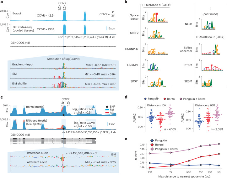
“When running MoDISco on gradients from tissue-pooled exon-to-intron coverage ratios for genes from the Gasperini set58, we found known splice-regulatory motifs (Fig. 7b).”
§ Predicting RNA-seq coverage from DNA sequence as a unifying model of gene regulation > Results > Functional splicing variant interpretation
What the sources say
- Supportedcites [58] Gasperini, M. et al. A genome-wide framework for mapping gene regulation via cellular genetic screens. Cell 176, 377–390.e19 (2019). source
The citation is attached to “genes from the Gasperini set,” not to the citing authors’ MoDISco result. The Results section identifies 353 target genes in the paper’s high-confidence enhancer–gene pairs, supporting the citation as identification of a gene set. No page number is available in our copy. (LLM, conf=0.91)
plaincorrelational- Asserted: passes — The authors put it forward as true.
- Checkable: passes — It can be checked against evidence.
- Load-bearing: passes — The paper’s conclusions depend on it.
- Based: passes — The paper gives a reason why it holds.
- The authors state this as an assumption: The inverse transforms applied to Borzoi's raw predictions yield a tensor that can be reasonably assumed to reflect counts.
- Supported
- Probably not a substantial claim. 49
- It may state two separate claims as one. 28
- The quote only partly states this claim. 1
The cited sources support only part of this claim — read each source’s verdict below.
In the paper
“Machine-learning models trained to predict function from DNA sequences have been successful at characterizing regulatory syntax and interpreting genetic variant effects.”
§ Predicting RNA-seq coverage from DNA sequence as a unifying model of gene regulation > Main
What the sources say
- Not checked — no full text of the sourcecites [4] Alipanahi, B., Delong, A., Weirauch, M. T. & Frey, B. J. Predicting the sequence specificities of DNA- and RNA-binding proteins by deep learning. Nat. Biotechnol. 33, 831–838 (2015). source
- Supportedcites [5] Zhou, J. & Troyanskaya, O. G. Predicting effects of noncoding variants with deep learning-based sequence model. Nat. Methods 12, 931–934 (2015). source
The Abstract (page not provided) says DeepSEA learns a regulatory sequence code from DNA to predict chromatin features. It also reports accurate predictions of single-nucleotide variant effects and improved prioritization of functional variants, supporting both parts of the claim. (LLM, conf=0.90)
- Supportedcites [6] Kelley, D. R., Snoek, J. & Rinn, J. L. Basset: learning the regulatory code of the accessible genome with deep convolutional neural networks. Genome Res. 26, 990–999 (2016). source
The Results section, “Basset recovers known protein binding motifs” (page unavailable), describes sequence motifs and surrounding features that influence the model’s predictions, supporting the regulatory-syntax point. The Results section, “Basset predicts greater accessibility changes for likely causal GWAS SNPs” (page unavailable), reports a variant whose predicted accessibility effect is supported by allele-specific binding data. (LLM, conf=0.91)
- Partly supportedcites [7] Avsec, Ž. et al. Base-resolution models of transcription-factor binding reveal soft motif syntax. Nat. Genet. 53, 354–366 (2021). sourceExperimental — accuracy not yet measured
The Abstract and Discussion show that BPNet uses DNA sequence to characterize regulatory motif syntax and predict the effects of experimentally introduced sequence changes. But the Discussion presents pinpointing disease-associated genetic variants as a future opportunity, not an accomplished interpretation of genetic variant effects in this study. (LLM, conf=0.85)
- Supportedcites [8] Kelley, D. R. et al. Sequential regulatory activity prediction across chromosomes with convolutional neural networks. Genome Res. 28, 739–750 (2018). source
The Abstract says that machine-learning models of DNA sequence have provided mechanistic insight and useful interpretation of genomic variants. The Results (Distal regulatory elements) also show the model identifying regulatory motifs, supporting the characterization of regulatory syntax. (LLM, conf=0.91)
- Supportedcites [9] Kelley, D. R. Cross-species regulatory sequence activity prediction. PLoS Comput. Biol. 16, e1008050 (2020). source
The Introduction says sequence-based machine-learning models have achieved significant accuracy gains and have been used to study genetic variation and propose mechanisms for noncoding variant effects. It also describes this paper’s models as learning regulatory grammars; the Abstract says such models have revealed principles of gene regulation and guided genetic variation analysis. (LLM, conf=0.92)
- Supportedcites [10] Chen, K. M., Wong, A. K., Troyanskaya, O. G. & Zhou, J. A sequence-based global map of regulatory activity for deciphering human genetics. Nat. Genet. 54, 940–949 (2022). source
The Main section (page not provided) says deep-learning sequence models have successfully learned features predictive of transcription-factor binding and histone modifications, and describes their use in inferring the effects of sequence variation. The Discussion (page not provided) also reports that the paper’s sequence-based model provides insights into the regulatory effects of individual mutations. (LLM, conf=0.90)
plaincorrelational- Asserted: passes — The authors put it forward as true.
- Checkable: passes — It can be checked against evidence.
- Load-bearing: passes — The paper’s conclusions depend on it.
- Based: passes — The paper gives a reason why it holds.
Probably not a substantial claim. It may state two separate claims as one.
The cited sources that could be checked couldn’t confirm or dispute this claim.
In the paper
“For example, RWDD1 exhibits biased usage of the distal-most PAS in brain42 (Fig. 2e; see Extended Data Fig. 3b for additional examples).”
§ Predicting RNA-seq coverage from DNA sequence as a unifying model of gene regulation > Results > Inference of tissue-specific expression and isoform usage
What the sources say
- Could not verifycites [42] Herrmann, C. J. et al. PolyASite 2.0: a consolidated atlas of polyadenylation sites from 3′ end sequencing. Nucleic Acids Res. 48, D174–D179 (2020). sourceExperimental — accuracy not yet measured
The Introduction describes PolyASite’s per-sample poly(A)-site usage data, but does not report a result for RWDD1 in brain. Searches for “RWDD1,” “brain,” and distal-site usage found no passage in our copy addressing the claimed bias. (LLM, conf=0.76)
plaincorrelational- Asserted: passes — The authors put it forward as true.
- Checkable: passes — It can be checked against evidence.
- Load-bearing: fails — The paper’s conclusions may not depend on it.
- Based: passes — The paper gives a reason why it holds.
Probably not a substantial claim. The paper’s conclusions may not depend on it.
- Could not verify
The sources with a verdict support this claim; the rest weren’t checked yet, have no full text we could read, or their verdicts aren’t rated yet.
In the paper
“Genes often have alternative TSSs, which are differentially used across tissues36–38.”
§ Predicting RNA-seq coverage from DNA sequence as a unifying model of gene regulation > Results > Inference of tissue-specific expression and isoform usage
What the sources say
- Not checked yetcites [36] Kimura, K. et al. Diversification of transcriptional modulation: large-scale identification and characterization of putative alternative promoters of human genes. Genome Res. 16, 55–65 (2006). source
Checked before — its earlier verdict is held back until a new check runs.
- Not checked — no full text of the sourcecites [37] de Klerk, E. & AC’t Hoen, P. Alternative mRNA transcription, processing, and translation: insights from RNA sequencing. Trends Genet. 31, 128–139 (2015). source
- Supportedcites [38] Reyes, A. & Huber, W. Alternative start and termination sites of transcription drive most transcript isoform differences across human tissues. Nucleic Acids Res. 46, 582–592 (2018). source
The Results section, “Analysis of CAGE data confirms prevalent tissue-dependent usage of alternative transcription start sites,” states that alternative TSSs are abundant and used in a tissue-dependent manner. It also reports thousands of genes with differential TSS usage across the examined cell-type subsets. (LLM, conf=0.94)
plaincorrelational- Asserted: passes — The authors put it forward as true.
- Checkable: passes — It can be checked against evidence.
- Load-bearing: fails — The paper’s conclusions may not depend on it.
- Based: passes — The paper gives a reason why it holds.
Probably not a substantial claim. The paper’s conclusions may not depend on it. It may state two separate claims as one.
- Not checked yet
The sources with a verdict support this claim; the rest weren’t checked yet, have no full text we could read, or their verdicts aren’t rated yet.
In the paper
“The 3′ untranslated region (UTR) harbors regulatory regions called polyadenylation signals (PASs), which can generate multiple isoforms with distinct 3′ ends through alternative polyadenylation (APA)39–41.”
§ Predicting RNA-seq coverage from DNA sequence as a unifying model of gene regulation > Results > Inference of tissue-specific expression and isoform usage
What the sources say
- Not checked yetcites [39] Colgan, D. F. & Manley, J. L. Mechanism and regulation of mRNA polyadenylation. Genes Dev. 11, 2755–2766 (1997). source
Checked before — its earlier verdict is held back until a new check runs.
- Supportedcites [40] Tian, B. & Manley, J. L. Alternative polyadenylation of mRNA precursors. Nat. Rev. Mol. Cell Biol. 18, 18–30 (2017). source
The “APA in 3′ UTRs” section states that most APA sites are in 3′ UTRs, identifies a proximal polyadenylation signal (PAS), and says that 3′ UTR-APA produces mRNA isoforms with different 3′ UTR lengths. This supports the attributed description of isoforms with distinct 3′ ends. (LLM, conf=0.93)
- Not checked yetcites [41] Shi, Y. Alternative polyadenylation: new insights from global analyses. RNA 18, 2105–2117 (2012). source
Checked before — its earlier verdict is held back until a new check runs.
plaindirect- Asserted: passes — The authors put it forward as true.
- Checkable: passes — It can be checked against evidence.
- Load-bearing: passes — The paper’s conclusions depend on it.
- Based: passes — The paper gives a reason why it holds.
Probably not a substantial claim.
- Not checked yet
Every source the paper cites for this claim was checked and supports it.
In the paper
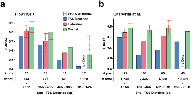
“In line with recent work66, we find a general decreasing trend in average predicted percent expression change with TSS distance for both positive and negative examples (Supplementary Fig. 6a).”
§ Predicting RNA-seq coverage from DNA sequence as a unifying model of gene regulation > Results > Improved context use for gene expression prediction
What the sources say
- Supportedcites [66] Karollus, A., Mauermeier, T. & Gagneur, J. Current sequence-based models capture gene expression determinants in promoters but mostly ignore distal enhancers. Genome Biol. 24, 56 (2023). source
The Results section (“Most distal eQTLs do not have a meaningful impact on expression predictions”; page unavailable) reports that Enformer’s predicted expression effects decrease rapidly as distance from the TSS increases. The cited work supports the distance trend; the positive- and negative-example breakdown is presented as the citing authors’ own finding. (LLM, conf=0.88)
plaincorrelational- Asserted: passes — The authors put it forward as true.
- Checkable: passes — It can be checked against evidence.
- Load-bearing: fails — The paper’s conclusions may not depend on it.
- Based: passes — The paper gives a reason why it holds.
Probably not a substantial claim. The paper’s conclusions may not depend on it.
- Supported
Every source the paper cites for this claim was checked and supports it.
In the paper
“Compared to Enformer13, Borzoi can score sites that are up to twice as far away from the gene, 262 kb, and we make use of exon annotations rather than TSS annotations, which are generally more robust to alternative isoforms.”
§ Predicting RNA-seq coverage from DNA sequence as a unifying model of gene regulation > Results > Improved context use for gene expression prediction
What the sources say
- Supportedcites [13] Avsec, Ž. et al. Effective gene expression prediction from sequence by integrating long-range interactions. Nat. Methods 18, 1196–1203 (2021). source
The citation is attached to Enformer as the comparator, not to the citing authors’ claims about Borzoi. In Results (Fig. 1a), the paper describes Enformer detecting elements 100 kb away; Methods (Model training and evaluation) describes using TSS locations for gene-expression predictions. These support the Enformer characteristics invoked by the comparison. (LLM, conf=0.86)
plaincorrelational- Asserted: passes — The authors put it forward as true.
- Checkable: passes — It can be checked against evidence.
- Load-bearing: passes — The paper’s conclusions depend on it.
- Based: passes — The paper gives a reason why it holds.
It may state two separate claims as one.
- Supported
The cited sources that could be checked couldn’t confirm or dispute this claim.
In the paper
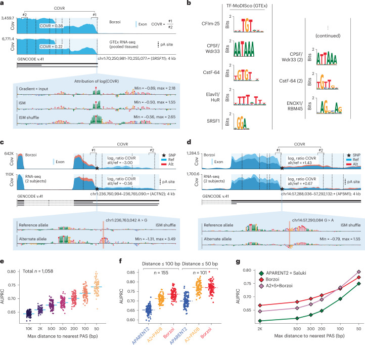
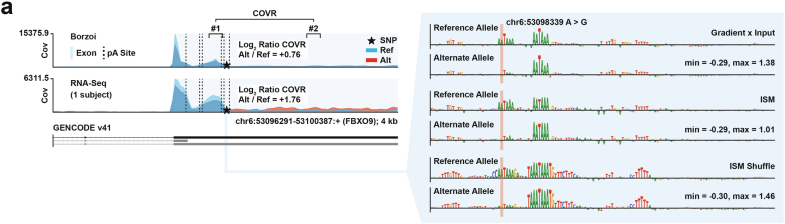
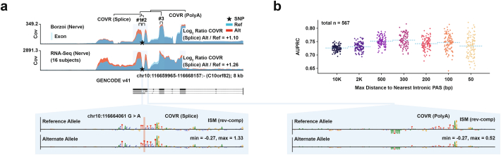
“Borzoi performs better at longer distances (dAUPRC > 0.050 at 2,000 bp) with a more comparable performance closer to the PAS (dAUPRC = 0.025 at 50 bp) (Fig. 6g).”
§ Predicting RNA-seq coverage from DNA sequence as a unifying model of gene regulation > Results > Functional polyadenylation variant interpretation
What the sources say
- Could not verifycites [23] Agarwal, V. & Kelley, D. R. The genetic and biochemical determinants of mRNA degradation rates in mammals. Genome Biol. 23, 245 (2022). sourceExperimental — accuracy not yet measured
The Results section on 3′ UTR regulatory function reports Saluki’s performance against experimental data, and its Fig. 6 caption describes panels a–e. Our copy does not address a Borzoi comparison or the stated dAUPRC values at 2,000 bp and 50 bp (searched: Borzoi, APARENT2, dAUPRC, and PAS distance). (LLM, conf=0.78)
plaincorrelational- Asserted: passes — The authors put it forward as true.
- Checkable: passes — It can be checked against evidence.
- Load-bearing: passes — The paper’s conclusions depend on it.
- Based: passes — The paper gives a reason why it holds.
It may state two separate claims as one.
- Could not verify
Every source the paper cites for this claim was checked and supports it.
In the paper
“The model is based on the Enformer network architecture but introduces a number of simplifications and enhancements to optimize for RNA-seq prediction13.”
§ Predicting RNA-seq coverage from DNA sequence as a unifying model of gene regulation > Methods > Model
What the sources say
- Supportedcites [13] Avsec, Ž. et al. Effective gene expression prediction from sequence by integrating long-range interactions. Nat. Methods 18, 1196–1203 (2021). source
The Methods section (‘Model architecture’) describes the Enformer network architecture, which is what the citation identifies as the basis for the citing authors’ model. The simplifications and enhancements for RNA-seq prediction describe the citing authors’ model, not a finding attributed to this source. (LLM, conf=0.90)
plain- Asserted: passes — The authors put it forward as true.
- Checkable: passes — It can be checked against evidence.
- Load-bearing: fails — The paper’s conclusions may not depend on it.
- Based: passes — The paper gives a reason why it holds.
Probably not a substantial claim. The paper’s conclusions may not depend on it. It may state two separate claims as one.
- Supported
The sources with a verdict support this claim; the rest weren’t checked yet, have no full text we could read, or their verdicts aren’t rated yet.
In the paper
“Identifying splice sites in DNA sequences has formed the basis for a successful approach to interpreting the splicing code and prioritizing pathogenic splicing variants15,16.”
§ Predicting RNA-seq coverage from DNA sequence as a unifying model of gene regulation > Methods > Splice site identification task
What the sources say
- Not checked — no full text of the sourcecites [15] Jaganathan, K. et al. Predicting splicing from primary sequence with deep learning. Cell 176, 535–548.e24 (2019). source
- Supportedcites [16] Zeng, T. & Li, Y. I. Predicting RNA splicing from DNA sequence using Pangolin. Genome Biol. 23, 103 (2022). source
The paper’s discussion of Pangolin’s applications (indexed under Supplementary Information; page unavailable) reports that it predicts splice-site usage from DNA sequence and helps pinpoint variants responsible for changes in that usage. The same section reports that it distinguished pathogenic from benign ClinVar splice-region variants and identified variants of uncertain significance likely to affect splicing. Together, these support the claimed approach to interpreting splicing and prioritizing pathogenic variants. (LLM, conf=0.88)
plaindirect- Asserted: passes — The authors put it forward as true.
- Checkable: passes — It can be checked against evidence.
- Load-bearing: fails — The paper’s conclusions may not depend on it.
- Based: passes — The paper gives a reason why it holds.
Probably not a substantial claim. The paper’s conclusions may not depend on it.
Every source the paper cites for this claim was checked and supports it.
In the paper
“which solve an analogous problem of determining image-level content and communicating it back down to pixel resolution annotations.”
§ Predicting RNA-seq coverage from DNA sequence as a unifying model of gene regulation > Methods > Model
What the sources say
- Supportedcites [29] Lin, T. Y. et al. Feature pyramid networks for object detection. In Proc. IEEE Conference on Computer Vision and Pattern Recognition (CVPR 2017) 936–944 (IEEE, 2017). source
Related Work (p. 3) identifies U-Net as a segmentation method using connections across resolutions and semantic levels. The Introduction (p. 2) describes similar top-down architectures as producing a fine-resolution feature map for predictions, supporting the claim's description of conveying high-level content back toward fine-resolution annotations. (LLM, conf=0.85)
- Supportedcites [30] Ronneberger, O., Fischer, P. & Brox, T. U-net: convolutional networks for biomedical image segmentation. In Medical Image Computing and Computer-Assisted Intervention (MICCAI 2015): Proc. 18th International Conference (eds Navab, N. et al.) 234–241 (Springer, 2015). source
The Introduction (p. 1) describes the goal as assigning a class label to each pixel. It explains that U-Net’s upsampling path propagates context information to higher-resolution layers (p. 3), supporting the claim’s description of communicating image context back to pixel-level annotations. (LLM, conf=0.90)
plaindirect- Asserted: passes — The authors put it forward as true.
- Checkable: passes — It can be checked against evidence.
- Load-bearing: fails — The paper’s conclusions may not depend on it.
- Based: passes — The paper gives a reason why it holds.
Probably not a substantial claim. The paper’s conclusions may not depend on it.
- Supported
Every source the paper cites for this claim was checked and supports it.
In the paper
“Prior work has demonstrated strong relationships between codon usage and mRNA half-life23,78.”
§ Predicting RNA-seq coverage from DNA sequence as a unifying model of gene regulation > Methods > Codon stability comparison
What the sources say
- Supportedcites [23] Agarwal, V. & Kelley, D. R. The genetic and biochemical determinants of mRNA degradation rates in mammals. Genome Biol. 23, 245 (2022). source
The Results section ('A genetic model of mRNA half-life'; page unavailable) describes established associations between codon frequencies and mRNA half-lives and uses those frequencies to predict half-life. The deep-learning Results section also calls the link mechanistic. Its reported correlation of 0.68 is between predicted codon effects and codon stability coefficients, not directly between codon usage and half-life. (LLM, conf=0.87)
- Supportedcites [78] Forrest, M. E. et al. Codon and amino acid content are associated with mRNA stability in mammalian cells. PLoS ONE 15, e0228730 (2020). source
The Discussion states that changing synonymous codon content alters human mRNA half-lives and that codon content is significantly associated with observed half-lives. The Results section reports significant associations between specific codons and transcript stability in mammalian cells. These passages support the cited statement about a strong relationship between codon usage and mRNA half-life. (LLM, conf=0.91)
boostedcorrelationaln = 3- Asserted: passes — The authors put it forward as true.
- Checkable: passes — It can be checked against evidence.
- Load-bearing: fails — The paper’s conclusions may not depend on it.
- Based: passes — The paper gives a reason why it holds.
Probably not a substantial claim. The paper’s conclusions may not depend on it.
- Supported
Every source the paper cites for this claim was checked and supports it.
In the paper
“which we reasoned would help the model relate TSS usage and strength to RNA-seq coverage between multiple (alternative) TSSs97,98”
§ Predicting RNA-seq coverage from DNA sequence as a unifying model of gene regulation > Methods > Training data
What the sources say
- Supportedcites [97] Noguchi, S. et al. FANTOM5 CAGE profiles of human and mouse samples. Sci. Data 4, 170112 (2017). source
The Background & Summary says CAGE monitors the frequency of transcription initiation by determining capped RNA 5′ ends. The Methods sections describe counting CAGE tag start sites and quantifying promoter activity, supporting its use for TSS location, usage and strength. The proposed relationship to RNA-seq coverage is the citing authors’ reasoning about their model, not a finding attributed to this paper. (LLM, conf=0.88)
- Supportedcites [98] Lizio, M. et al. Gateways to the FANTOM5 promoter level mammalian expression atlas. Genome Biol. 16, 22 (2015). source
The Introduction says CAGE quantifies TSS activity at single-base resolution. In Materials and methods, the paper describes ranking multiple CAGE peaks associated with one gene by their counts and quantifying each region’s activity. The proposed relationship to RNA-seq coverage is the citing authors’ own reasoning, not a result attributed to this source. (LLM, conf=0.87)
hedgedcorrelational- Asserted: passes — The authors put it forward as true.
- Checkable: passes — It can be checked against evidence.
- Load-bearing: passes — The paper’s conclusions depend on it.
- Based: passes — The paper gives a reason why it holds.
Probably not a substantial claim.
- Supported
Every source the paper cites for this claim was checked and supports it.
In the paper
“To reduce the risk of picking genes in which the perceived APA is driven by 3′ bias in the GTEx RNA-seq data, we required that the genes also exhibited differential distal polyadenylation in cell-type-matched experiments from the PolyASite 2.0 database42.”
§ Predicting RNA-seq coverage from DNA sequence as a unifying model of gene regulation > Methods > Tissue-specific expression, TSS and APA predictions
What the sources say
- Supportedcites [42] Herrmann, C. J. et al. PolyASite 2.0: a consolidated atlas of polyadenylation sites from 3′ end sequencing. Nucleic Acids Res. 48, D174–D179 (2020). source
The citation identifies PolyASite 2.0 as the source of the experiments, not as the source of the citing authors’ selection rule. The Introduction describes data covering many cell types and conditions, and Results > Website roadmap says the database provides sample-specific poly(A)-site abundances and cell-type information. Those passages support its use for the stated comparison; the requirement imposed on genes is the citing authors’ own method. (LLM, conf=0.90)
plaindirect- Asserted: passes — The authors put it forward as true.
- Checkable: passes — It can be checked against evidence.
- Load-bearing: passes — The paper’s conclusions depend on it.
- Based: passes — The paper gives a reason why it holds.
Probably not a substantial claim.
- Supported
Every source the paper cites for this claim was checked and supports it.
In the paper
“as well as DNase-seq and ChIP–seq from ENCODE and the Epigenomics Roadmap31,99 and pseudo-bulk single-cell ATAC–seq data from CATlas100,101, which focuses the model towards distal regulatory elements.”
§ Predicting RNA-seq coverage from DNA sequence as a unifying model of gene regulation > Methods > Training data
What the sources say
- Supportedcites [31] ENCODE Project Consortium. An integrated encyclopedia of DNA elements in the human genome. Nature 489, 57–74 (2012). source
The ENCODE data production and initial analyses section states that ENCODE used both DNase-seq and ChIP-seq to map functional elements. Its DNaseI hypersensitive sites section reports that the overwhelming majority of mapped sites lie distal to transcription start sites. The Roadmap and CATlas data and the effect on the citing authors’ model are not attributed to this ENCODE paper. (LLM, conf=0.90)
- Supportedcites [99] Roadmap Epigenomics Consortium et al. Integrative analysis of 111 reference human epigenomes. Nature 518, 317–330 (2015). source
The Introduction says the Roadmap reference epigenomes used ChIP and DNase assays followed by sequencing. Online Methods §1.2 explicitly describes ChIP-seq and DNase-seq processing. The CATlas data and the citing authors’ model are not attributed to this source. (LLM, conf=0.92)
- Supportedcites [100] Zhang, K. et al. A single-cell atlas of chromatin accessibility in the human genome. Cell 184, 5985–6001.e19 (2021). source
The Introduction (page unavailable) identifies this paper’s single-cell ATAC-seq resource as CATLAS. The Results section (page unavailable) says the authors aggregated accessibility profiles from nuclei within each cell cluster, supporting the description of pseudo-bulk data. The statement about focusing the citing authors’ model toward distal regulatory elements is their own framing, not a finding attributed to this source. (LLM, conf=0.92)
- Supportedcites [101] Li, Y. E. et al. A comparative atlas of single-cell chromatin accessibility in the human brain. Science 382, eadf7044 (2023). source
The paper’s Abstract identifies its single-cell chromatin accessibility atlas as CATLAS and says it maps candidate cis-regulatory elements in human brain cell types. This supports the citation’s identification of CATLAS as the source of the ATAC-seq data. The statement about focusing the citing authors’ model toward distal elements describes their use of those data, not a result attributed to this paper. (LLM, conf=0.91)
plaindirect- Asserted: passes — The authors put it forward as true.
- Checkable: passes — It can be checked against evidence.
- Load-bearing: fails — The paper’s conclusions may not depend on it.
- Based: passes — The paper gives a reason why it holds.
Probably not a substantial claim. The paper’s conclusions may not depend on it.
- Supported
A result the paper reports from its own data — it cites no other source for it, so there is none to check. The quote shows it is in the paper.
In the paper
“Evaluated on quantitative trait loci, Borzoi is competitive with and often outperforms state-of-the-art models trained on individual regulatory functions.”
§ Predicting RNA-seq coverage from DNA sequence as a unifying model of gene regulation > Abstract
plain- Asserted: passes — The authors put it forward as true.
- Checkable: passes — It can be checked against evidence.
- Load-bearing: passes — The paper’s conclusions depend on it.
- Based: passes — The paper gives a reason why it holds.
It may state two separate claims as one.
The paper states this without a source or data behind it here, so there is nothing to check it against. The quote shows it is in the paper.
In the paper
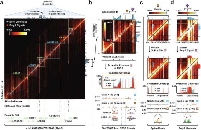
“By applying attribution methods to predicted coverage patterns of individual RNA-seq experiments present in the training data, Borzoi derives the primary cell-type-specific or state-specific TF motifs and a genome-wide map of nucleotide influence on gene structure and expression.”
§ Predicting RNA-seq coverage from DNA sequence as a unifying model of gene regulation > Main
plaindirect- Asserted: passes — The authors put it forward as true.
- Checkable: passes — It can be checked against evidence.
- Load-bearing: passes — The paper’s conclusions depend on it.
- Based: passes — The paper gives a reason why it holds.
It may state two separate claims as one.
A result the paper reports from its own data — it cites no other source for it, so there is none to check. The quote shows it is in the paper.
In the paper
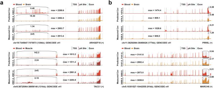
“We computed TSS usage ratios for the 5′-most and 3′-most TSSs from our ensembled predictions (Methods) and found correlations with experimental measurements (Spearman’s R = 0.85; Supplementary Fig. 3c), FANTOM5 TSS usage proportions (Supplementary Fig. 3d) and tissue-specific TSS usage ratio fold changes (Spearman’s R = 0.29−0.50 on held-out genes; Fig. 2d and Supplementary Fig. 3e).”
§ Predicting RNA-seq coverage from DNA sequence as a unifying model of gene regulation > Results > Inference of tissue-specific expression and isoform usage
plaincorrelational- Asserted: passes — The authors put it forward as true.
- Checkable: passes — It can be checked against evidence.
- Load-bearing: passes — The paper’s conclusions depend on it.
- Based: passes — The paper gives a reason why it holds.
It may state two separate claims as one.
A result the paper reports from its own data — it cites no other source for it, so there is none to check. The quote shows it is in the paper.
In the paper
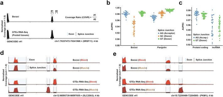
“In the Supplementary Information, we show that although Borzoi competitively identifies splice junctions from matched negatives, the model has not learned to predict alternative splicing across tissues well (Extended Data Fig. 4; see Discussion).”
§ Predicting RNA-seq coverage from DNA sequence as a unifying model of gene regulation > Results > Inference of tissue-specific expression and isoform usage
plain- Asserted: passes — The authors put it forward as true.
- Checkable: passes — It can be checked against evidence.
- Load-bearing: unclear — It is unclear whether the paper’s conclusions depend on it.
- Based: passes — The paper gives a reason why it holds.
It may state two separate claims as one.
A result the paper reports from its own data — it cites no other source for it, so there is none to check. The quote shows it is in the paper.
In the paper
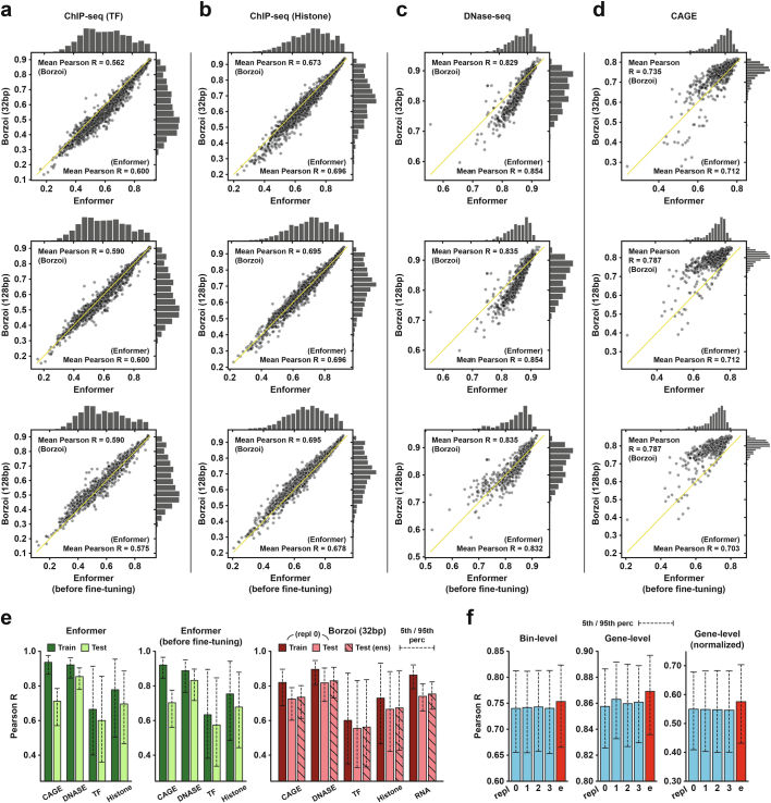
“Nevertheless, test accuracies on overlapping datasets are broadly similar (Extended Data Fig. 1a–e) with two exceptions: the average Pearson’s R is lower than Enformer for DNase and higher for CAGE.”
§ Predicting RNA-seq coverage from DNA sequence as a unifying model of gene regulation > Results > Borzoi accurately predicts RNA-seq and other assays
plain- Asserted: passes — The authors put it forward as true.
- Checkable: passes — It can be checked against evidence.
- Load-bearing: unclear — It is unclear whether the paper’s conclusions depend on it.
- Based: passes — The paper gives a reason why it holds.
It may state two separate claims as one.
A result the paper reports from its own data — it cites no other source for it, so there is none to check. The quote shows it is in the paper.
In the paper
“most tissue-specific splicing events were not captured well by the model, which rather tended to predict the average RNA-seq shape.”
§ Predicting RNA-seq coverage from DNA sequence as a unifying model of gene regulation > Discussion
plain- Asserted: passes — The authors put it forward as true.
- Checkable: passes — It can be checked against evidence.
- Load-bearing: unclear — It is unclear whether the paper’s conclusions depend on it.
- Based: passes — The paper gives a reason why it holds.
It may state two separate claims as one.
A result the paper reports from its own data — it cites no other source for it, so there is none to check. The quote shows it is in the paper.
In the paper
“We found that the gradient scores were broadly similar across replicates and closely matched in-silico saturation mutagenesis (ISM) (Supplementary Fig. 4).”
§ Predicting RNA-seq coverage from DNA sequence as a unifying model of gene regulation > Results > Borzoi identifies regulatory motifs driving RNA expression
plaincorrelational- Asserted: passes — The authors put it forward as true.
- Checkable: passes — It can be checked against evidence.
- Load-bearing: unclear — It is unclear whether the paper’s conclusions depend on it.
- Based: passes — The paper gives a reason why it holds.
It may state two separate claims as one.
A result the paper reports from its own data — it cites no other source for it, so there is none to check. The quote shows it is in the paper.
In the paper
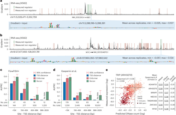
“Fig. 4a,b displays the gradient attributions for genes HBE1 and MYC, in which Borzoi correctly identifies both proximal (distance to TSS, <20,000 bp) and distal (distance to TSS, >200,000) enhancers, although false positives are also present.”
§ Predicting RNA-seq coverage from DNA sequence as a unifying model of gene regulation > Results > Improved context use for gene expression prediction
plain- Asserted: passes — The authors put it forward as true.
- Checkable: passes — It can be checked against evidence.
- Load-bearing: passes — The paper’s conclusions depend on it.
- Based: passes — The paper gives a reason why it holds.
It may state two separate claims as one.
A result the paper reports from its own data — it cites no other source for it, so there is none to check. The quote shows it is in the paper.
In the paper
“Importantly, the average rank prediction of both models is superior to either model alone (dAUPRC > 0.02).”
§ Predicting RNA-seq coverage from DNA sequence as a unifying model of gene regulation > Results > Functional splicing variant interpretation
plaincorrelational- Asserted: passes — The authors put it forward as true.
- Checkable: passes — It can be checked against evidence.
- Load-bearing: unclear — It is unclear whether the paper’s conclusions depend on it.
- Based: passes — The paper gives a reason why it holds.
The quote only partly states this claim.
A result the paper reports from its own data — it cites no other source for it, so there is none to check. The quote shows it is in the paper.
In the paper
“Borzoi still outperformed Enformer when using a single model (AUROC = 0.788) or when switching to the original sum statistic (AUROC = 0.772).”
§ Predicting RNA-seq coverage from DNA sequence as a unifying model of gene regulation > Results > Borzoi prioritizes genetic variants that influence expression
plaincorrelational- Asserted: passes — The authors put it forward as true.
- Checkable: passes — It can be checked against evidence.
- Load-bearing: passes — The paper’s conclusions depend on it.
- Based: passes — The paper gives a reason why it holds.
It may state two separate claims as one.
The paper states this without a source or data behind it here, so there is nothing to check it against. The quote shows it is in the paper.
In the paper
“When averaging predictions across an ensemble of model replicates, Borzoi’s performance improved further.”
§ Predicting RNA-seq coverage from DNA sequence as a unifying model of gene regulation > Discussion
plaindirect- Asserted: passes — The authors put it forward as true.
- Checkable: passes — It can be checked against evidence.
- Load-bearing: fails — The paper’s conclusions may not depend on it.
- Based: passes — The paper gives a reason why it holds.
Probably not a substantial claim. The paper’s conclusions may not depend on it.
A result the paper reports from its own data — it cites no other source for it, so there is none to check. The quote shows it is in the paper.
In the paper
“Smaller or larger window sizes only marginally affected the results (as shown in Supplementary Fig. 7a).”
§ Predicting RNA-seq coverage from DNA sequence as a unifying model of gene regulation > Methods > Gene–enhancer prioritization task
plain- Asserted: passes — The authors put it forward as true.
- Checkable: passes — It can be checked against evidence.
- Load-bearing: fails — The paper’s conclusions may not depend on it.
- Based: passes — The paper gives a reason why it holds.
Probably not a substantial claim. The paper’s conclusions may not depend on it.
The paper states this without a source or data behind it here, so there is nothing to check it against. The quote shows it is in the paper.
In the paper
“Computing the gradient using three bins (as in the original paper) resulted in marginally worse performance.”
§ Predicting RNA-seq coverage from DNA sequence as a unifying model of gene regulation > Methods > Gene–enhancer prioritization task
plaindirect- Asserted: passes — The authors put it forward as true.
- Checkable: passes — It can be checked against evidence.
- Load-bearing: fails — The paper’s conclusions may not depend on it.
- Based: passes — The paper gives a reason why it holds.
Probably not a substantial claim. The paper’s conclusions may not depend on it.
A result the paper reports from its own data — it cites no other source for it, so there is none to check. The quote shows it is in the paper.
In the paper
“We further noted that different attention heads tended to capture mostly the same trends, leading us to analyze the mean attention of all eight heads.”
§ Predicting RNA-seq coverage from DNA sequence as a unifying model of gene regulation > Methods > Attention matrix visualization
plaincorrelational- Asserted: passes — The authors put it forward as true.
- Checkable: passes — It can be checked against evidence.
- Load-bearing: fails — The paper’s conclusions may not depend on it.
- Based: passes — The paper gives a reason why it holds.
Probably not a substantial claim. The paper’s conclusions may not depend on it.
A result the paper reports from its own data — it cites no other source for it, so there is none to check. The quote shows it is in the paper.
In the paper
“Similarly, the average optimal CAGE window size was 8,813 bp, but the 4,096 bp window had near-identical performance (<0.01 difference in average Spearman’s R across promoter types).”
§ Predicting RNA-seq coverage from DNA sequence as a unifying model of gene regulation > Methods > Predicting TRIP expression
plain- Asserted: passes — The authors put it forward as true.
- Checkable: passes — It can be checked against evidence.
- Load-bearing: unclear — It is unclear whether the paper’s conclusions depend on it.
- Based: passes — The paper gives a reason why it holds.
It may state two separate claims as one.
A result the paper reports from its own data — it cites no other source for it, so there is none to check. The quote shows it is in the paper.
In the paper
“The flow/proliferation dataset contains 117 positives out of 2,194 tested within 262 kb of the gene’s TSS.”
§ Predicting RNA-seq coverage from DNA sequence as a unifying model of gene regulation > Methods > Gene–enhancer prioritization task
plain- Asserted: passes — The authors put it forward as true.
- Checkable: passes — It can be checked against evidence.
- Load-bearing: fails — The paper’s conclusions may not depend on it.
- Based: passes — The paper gives a reason why it holds.
Probably not a substantial claim. The paper’s conclusions may not depend on it.
The paper states this without a source or data behind it here, so there is nothing to check it against. The quote shows it is in the paper.
In the paper
“The gradient score statistic was averaged for genes with multiple TSSs, which performed better than taking either the max or sum.”
§ Predicting RNA-seq coverage from DNA sequence as a unifying model of gene regulation > Methods > Gene–enhancer prioritization task
plaincorrelational- Asserted: passes — The authors put it forward as true.
- Checkable: passes — It can be checked against evidence.
- Load-bearing: unclear — It is unclear whether the paper’s conclusions depend on it.
- Based: passes — The paper gives a reason why it holds.
It may state two separate claims as one.
A result the paper reports from its own data — it cites no other source for it, so there is none to check. The quote shows it is in the paper.
In the paper
“For a second genome-wide benchmark, we sampled uniformly from across the genome instead of restricting the variant sampling to ENCODE candidate cis-regulatory elements. This resulted in a variant set containing 17,360 singletons and 17,360 matched common variants.”
§ Predicting RNA-seq coverage from DNA sequence as a unifying model of gene regulation > Methods > Classifying rare and common variation from gnomAD
plaindirect- Asserted: passes — The authors put it forward as true.
- Checkable: passes — It can be checked against evidence.
- Load-bearing: fails — The paper’s conclusions may not depend on it.
- Based: passes — The paper gives a reason why it holds.
Probably not a substantial claim. The paper’s conclusions may not depend on it.
A result the paper reports from its own data — it cites no other source for it, so there is none to check. The quote shows it is in the paper.
In the paper
“Promoters generally had higher magnitude attention values than exons, leading us to clip individual entries in the average attention matrix at 0.005 (each row of 4,096 entries sums to 1.0).”
§ Predicting RNA-seq coverage from DNA sequence as a unifying model of gene regulation > Methods > Attention matrix visualization
plaincorrelational- Asserted: passes — The authors put it forward as true.
- Checkable: passes — It can be checked against evidence.
- Load-bearing: fails — The paper’s conclusions may not depend on it.
- Based: passes — The paper gives a reason why it holds.
Probably not a substantial claim. The paper’s conclusions may not depend on it.
The paper states this without a source or data behind it here, so there is nothing to check it against. The quote shows it is in the paper.
In the paper
“In summary, we developed a neural network model for predicting RNA coverage from sequence and demonstrated its performance on multiple variant interpretation tasks.”
§ Predicting RNA-seq coverage from DNA sequence as a unifying model of gene regulation > Discussion
boosted- Asserted: passes — The authors put it forward as true.
- Checkable: passes — It can be checked against evidence.
- Load-bearing: passes — The paper’s conclusions depend on it.
- Based: passes — The paper gives a reason why it holds.
It may state two separate claims as one.
A result the paper reports from its own data — it cites no other source for it, so there is none to check. The quote shows it is in the paper.
In the paper
“Using a narrow 512 bp window for aggregation as in the Enformer paper13 resulted in worse concordance with measured effects for some promoters and better concordance for other promoters.”
§ Predicting RNA-seq coverage from DNA sequence as a unifying model of gene regulation > Methods > Saturation mutagenesis MPRA benchmark
plaindirect- Asserted: passes — The authors put it forward as true.
- Checkable: passes — It can be checked against evidence.
- Load-bearing: unclear — It is unclear whether the paper’s conclusions depend on it.
- Based: passes — The paper gives a reason why it holds.
It may state two separate claims as one.
The paper states this without a source or data behind it here, so there is nothing to check it against. The quote shows it is in the paper.
In the paper
“These numbers shrunk further on a per-analysis basis after requiring that each enhancer–gene pair is within the input window of the current set of models evaluated in a given benchmark.”
§ Predicting RNA-seq coverage from DNA sequence as a unifying model of gene regulation > Methods > Gene–enhancer prioritization task
plaindirect- Asserted: passes — The authors put it forward as true.
- Checkable: passes — It can be checked against evidence.
- Load-bearing: fails — The paper’s conclusions may not depend on it.
- Based: passes — The paper gives a reason why it holds.
Probably not a substantial claim. The paper’s conclusions may not depend on it.
A result the paper reports from its own data — it cites no other source for it, so there is none to check. The quote shows it is in the paper.
In the paper
“For DNase and histone ChIP tracks, we used a slightly wider 8,192 bp window size as we noticed that the correlation to measured expression saturated less quickly than CAGE as a function of window size (for example, ~0.02 difference in average Spearman’s R across promoter types when comparing a window size of 4,096 bp to 8,192 bp for H3K4me3).”
§ Predicting RNA-seq coverage from DNA sequence as a unifying model of gene regulation > Methods > Predicting TRIP expression
plaincorrelational- Asserted: passes — The authors put it forward as true.
- Checkable: passes — It can be checked against evidence.
- Load-bearing: fails — The paper’s conclusions may not depend on it.
- Based: passes — The paper gives a reason why it holds.
Probably not a substantial claim. The paper’s conclusions may not depend on it.
A result the paper reports from its own data — it cites no other source for it, so there is none to check. The quote shows it is in the paper.
In the paper
“we end up with ~2.5× the amount of unique negative SNPs after merging across tissues”
§ Predicting RNA-seq coverage from DNA sequence as a unifying model of gene regulation > Methods > Fine-mapped paQTL classification task
plain- Asserted: passes — The authors put it forward as true.
- Checkable: passes — It can be checked against evidence.
- Load-bearing: fails — The paper’s conclusions may not depend on it.
- Based: passes — The paper gives a reason why it holds.
Probably not a substantial claim. The paper’s conclusions may not depend on it.
A result the paper reports from its own data — it cites no other source for it, so there is none to check. The quote shows it is in the paper.
In the paper
“We settled on the wider 4 kb window as it led to better performance on the majority of promoters.”
§ Predicting RNA-seq coverage from DNA sequence as a unifying model of gene regulation > Methods > Saturation mutagenesis MPRA benchmark
plaindirect- Asserted: passes — The authors put it forward as true.
- Checkable: passes — It can be checked against evidence.
- Load-bearing: fails — The paper’s conclusions may not depend on it.
- Based: passes — The paper gives a reason why it holds.
Probably not a substantial claim. The paper’s conclusions may not depend on it.
The paper states this without a source or data behind it here, so there is nothing to check it against. The quote shows it is in the paper.
In the paper
“We constructed an ensemble predictor from these four replicates that generally performed better than any individual model.”
§ Predicting RNA-seq coverage from DNA sequence as a unifying model of gene regulation > Methods > Training
hedgedcorrelational- Asserted: passes — The authors put it forward as true.
- Checkable: passes — It can be checked against evidence.
- Load-bearing: fails — The paper’s conclusions may not depend on it.
- Based: passes — The paper gives a reason why it holds.
Probably not a substantial claim. The paper’s conclusions may not depend on it.
A result the paper reports from its own data — it cites no other source for it, so there is none to check. The quote shows it is in the paper.
In the paper
“a narrow 128 bp window maximized the average Spearman’s R across promoters for RNA-seq”
§ Predicting RNA-seq coverage from DNA sequence as a unifying model of gene regulation > Methods > Predicting TRIP expression
plaincorrelational- Asserted: passes — The authors put it forward as true.
- Checkable: passes — It can be checked against evidence.
- Load-bearing: fails — The paper’s conclusions may not depend on it.
- Based: passes — The paper gives a reason why it holds.
Probably not a substantial claim. The paper’s conclusions may not depend on it.
A conclusion the paper draws from its own results — it cites no other source for it, so there is none to check. The quote shows it is in the paper.
In the paper
“However, the long span of mammalian genes means that we must also work with very long sequences to cover all exons and relevant regulatory elements.”
§ Predicting RNA-seq coverage from DNA sequence as a unifying model of gene regulation > Results > RNA-seq model design
plaindirect- Asserted: passes — The authors put it forward as true.
- Checkable: passes — It can be checked against evidence.
- Load-bearing: passes — The paper’s conclusions depend on it.
- Based: fails — The paper may give no reason why it holds.
Probably not a substantial claim. The paper may give no reason why it holds.
- Rests on an assumption: Mammalian genes often span hundreds of thousands of nucleotides.
The paper states this without a source or data behind it here, so there is nothing to check it against. The quote shows it is in the paper.
In the paper
“Other models predict cap analysis of gene expression (CAGE), which measures expression at the 5′ end of capped RNA (representing the TSS) and does not capture coverage at individual exons.”
§ Predicting RNA-seq coverage from DNA sequence as a unifying model of gene regulation > Main
plain- Asserted: passes — The authors put it forward as true.
- Checkable: passes — It can be checked against evidence.
- Load-bearing: passes — The paper’s conclusions depend on it.
- Based: passes — The paper gives a reason why it holds.
It may state two separate claims as one.
A conclusion the paper draws from its own results — it cites no other source for it, so there is none to check. The quote shows it is in the paper.
In the paper
“This approach depends on accurate TSS annotation and ignores isoform complexity.”
§ Predicting RNA-seq coverage from DNA sequence as a unifying model of gene regulation > Main
plaindirect- Asserted: passes — The authors put it forward as true.
- Checkable: passes — It can be checked against evidence.
- Load-bearing: passes — The paper’s conclusions depend on it.
- Based: passes — The paper gives a reason why it holds.
It may state two separate claims as one.
None of the sources cited for this claim have been checked yet.
In the paper
“Another important class of disease variants alters 3′ mRNA processing77.”
§ Predicting RNA-seq coverage from DNA sequence as a unifying model of gene regulation > Results > Functional polyadenylation variant interpretation
What the sources say
- Not checked yetcites [77] Danckwardt, S., Hentze, M. W. & Kulozik, A. E. 3′ end mRNA processing: molecular mechanisms and implications for health and disease. EMBO J. 27, 482–498 (2008). source
Checked before — its earlier verdict is held back until a new check runs.
plaindirect- Asserted: passes — The authors put it forward as true.
- Checkable: passes — It can be checked against evidence.
- Load-bearing: fails — The paper’s conclusions may not depend on it.
- Based: passes — The paper gives a reason why it holds.
Probably not a substantial claim. The paper’s conclusions may not depend on it.
- Not checked yet
A conclusion the paper draws from its own results — it cites no other source for it, so there is none to check. The quote shows it is in the paper.
In the paper
“The variant weakens an alternative 3′ splice site, which upregulates extension of the corresponding exon.”
§ Predicting RNA-seq coverage from DNA sequence as a unifying model of gene regulation > Results > Functional splicing variant interpretation
plaindirectn = 5- Asserted: passes — The authors put it forward as true.
- Checkable: passes — It can be checked against evidence.
- Load-bearing: unclear — It is unclear whether the paper’s conclusions depend on it.
- Based: passes — The paper gives a reason why it holds.
It may state two separate claims as one.
A conclusion the paper draws from its own results — it cites no other source for it, so there is none to check. The quote shows it is in the paper.
In the paper
“Most far-away SNPs are de novo splice–gain mutations and are relatively easy for Pangolin to classify based on the local predicted effect at the variant allele”
§ Predicting RNA-seq coverage from DNA sequence as a unifying model of gene regulation > Results > Functional splicing variant interpretation
plaindirectn = 4,105- Asserted: passes — The authors put it forward as true.
- Checkable: passes — It can be checked against evidence.
- Load-bearing: unclear — It is unclear whether the paper’s conclusions depend on it.
- Based: passes — The paper gives a reason why it holds.
It may state two separate claims as one.
A conclusion the paper draws from its own results — it cites no other source for it, so there is none to check. The quote shows it is in the paper.
In the paper
“This observation suggests that recent multiome datasets, which measure both accessibility and expression in single cells, would be valuable as joint training data.”
§ Predicting RNA-seq coverage from DNA sequence as a unifying model of gene regulation > Discussion
hedged- Asserted: passes — The authors put it forward as true.
- Checkable: fails — It may be too vague to check against evidence.
- Load-bearing: fails — The paper’s conclusions may not depend on it.
- Based: passes — The paper gives a reason why it holds.
Probably not a substantial claim. It may be too vague to check against evidence. The paper’s conclusions may not depend on it.
A conclusion the paper draws from its own results — it cites no other source for it, so there is none to check. The quote shows it is in the paper.
In the paper
“we either use methods based on gradient saliency, which are computationally efficient for single outputs but tend to be noisier owing to moving off the one-hot coding simplex, or in-silico mutagenesis, which often give better-calibrated attributions for all outputs, but are too computationally expensive to run on long sequences.”
§ Predicting RNA-seq coverage from DNA sequence as a unifying model of gene regulation > Methods > Input sequence attribution
plaindirect- Asserted: passes — The authors put it forward as true.
- Checkable: passes — It can be checked against evidence.
- Load-bearing: fails — The paper’s conclusions may not depend on it.
- Based: passes — The paper gives a reason why it holds.
Probably not a substantial claim. The paper’s conclusions may not depend on it. It may state two separate claims as one.
- The authors state this as an assumption: The inverse transforms applied to Borzoi's raw predictions yield a tensor that can be reasonably assumed to reflect counts.
What the paper did — it cites no source for this, so there is none to check. The quote shows it is in the paper.
In the paper
“All example genes were picked from the held-out test set, and coverage was predicted using the four-replicate ensemble.”
§ Predicting RNA-seq coverage from DNA sequence as a unifying model of gene regulation > Methods > Tissue-specific expression, TSS and APA predictions
plain- Asserted: passes — The authors put it forward as true.
- Checkable: passes — It can be checked against evidence.
- Load-bearing: fails — The paper’s conclusions may not depend on it.
- Based: passes — The paper gives a reason why it holds.
Probably not a substantial claim. The paper’s conclusions may not depend on it. It may state two separate claims as one.
What the paper did — it cites no source for this, so there is none to check. The quote shows it is in the paper.
In the paper
“No data were otherwise excluded from analyses.”
§ Predicting RNA-seq coverage from DNA sequence as a unifying model of gene regulation > Methods > Statistics and reproducibility
plain- Asserted: passes — The authors put it forward as true.
- Checkable: passes — It can be checked against evidence.
- Load-bearing: fails — The paper’s conclusions may not depend on it.
- Based: passes — The paper gives a reason why it holds.
Probably not a substantial claim. The paper’s conclusions may not depend on it.
A conclusion the paper draws from its own results — it cites no other source for it, so there is none to check. The quote shows it is in the paper.
In the paper
“Notably, a single distal credible set variant can inflate the minimum average distance statistic, resulting in an incorrect eGene prediction, whereas maximizing the inverse distance does not lead to this problem.”
§ Predicting RNA-seq coverage from DNA sequence as a unifying model of gene regulation > Methods > Fine-mapped eQTL classification and regression tasks
plaindirect- Asserted: passes — The authors put it forward as true.
- Checkable: passes — It can be checked against evidence.
- Load-bearing: passes — The paper’s conclusions depend on it.
- Based: passes — The paper gives a reason why it holds.
It may state two separate claims as one.
What the paper did — it cites no source for this, so there is none to check. The quote shows it is in the paper.
In the paper
“each bucket contained at least 100 genes”
§ Predicting RNA-seq coverage from DNA sequence as a unifying model of gene regulation > Methods > Fine-mapped paQTL classification task
plain- Asserted: passes — The authors put it forward as true.
- Checkable: passes — It can be checked against evidence.
- Load-bearing: fails — The paper’s conclusions may not depend on it.
- Based: passes — The paper gives a reason why it holds.
Probably not a substantial claim. The paper’s conclusions may not depend on it.
A conclusion the paper draws from its own results — it cites no other source for it, so there is none to check. The quote shows it is in the paper.
In the paper
“The relatively large number of fine-mapped causal sQTLs allows for a tissue-specific benchmark comparison.”
§ Predicting RNA-seq coverage from DNA sequence as a unifying model of gene regulation > Methods > Splicing variant effect prediction
plaindirect- Asserted: passes — The authors put it forward as true.
- Checkable: passes — It can be checked against evidence.
- Load-bearing: fails — The paper’s conclusions may not depend on it.
- Based: fails — The paper may give no reason why it holds.
Probably not a substantial claim. The paper’s conclusions may not depend on it. The paper may give no reason why it holds.
What the paper did — it cites no source for this, so there is none to check. The quote shows it is in the paper.
In the paper
“We tried varying the percentile threshold (from 1 to 100) and the results were robust to this parameter (the same motif clusters were identified with roughly the same number of supporting seqlets).”
§ Predicting RNA-seq coverage from DNA sequence as a unifying model of gene regulation > Methods > Tissue-pooled splice motif discovery
plain- Asserted: passes — The authors put it forward as true.
- Checkable: passes — It can be checked against evidence.
- Load-bearing: fails — The paper’s conclusions may not depend on it.
- Based: passes — The paper gives a reason why it holds.
Probably not a substantial claim. The paper’s conclusions may not depend on it.
A conclusion the paper draws from its own results — it cites no other source for it, so there is none to check. The quote shows it is in the paper.
In the paper
“Direct modeling of RNA-seq opens the door to studying a wide range of experimental assays, increasing our ability to understand the impact of genetic variation on gene-regulatory processes.”
§ Predicting RNA-seq coverage from DNA sequence as a unifying model of gene regulation > Discussion
plaindirect- Asserted: passes — The authors put it forward as true.
- Checkable: fails — It may be too vague to check against evidence.
- Load-bearing: fails — The paper’s conclusions may not depend on it.
- Based: passes — The paper gives a reason why it holds.
Probably not a substantial claim. It may be too vague to check against evidence. The paper’s conclusions may not depend on it.
What the paper did — it cites no source for this, so there is none to check. The quote shows it is in the paper.
In the paper
“The experiments were not randomized and the authors were not blinded to outcome assessment.”
§ Predicting RNA-seq coverage from DNA sequence as a unifying model of gene regulation > Methods > Statistics and reproducibility
plain- Asserted: passes — The authors put it forward as true.
- Checkable: passes — It can be checked against evidence.
- Load-bearing: fails — The paper’s conclusions may not depend on it.
- Based: passes — The paper gives a reason why it holds.
Probably not a substantial claim. The paper’s conclusions may not depend on it. It may state two separate claims as one.
What the paper did — it cites no source for this, so there is none to check. The quote shows it is in the paper.
In the paper
“Note that for all analyses in Figs. 1 and 2 in which we evaluate model performance, we do so strictly on fragments from the held-out test set.”
§ Predicting RNA-seq coverage from DNA sequence as a unifying model of gene regulation > Methods > Training
plain- Asserted: passes — The authors put it forward as true.
- Checkable: passes — It can be checked against evidence.
- Load-bearing: passes — The paper’s conclusions depend on it.
- Based: passes — The paper gives a reason why it holds.
Probably not a substantial claim.
What the paper did — it cites no source for this, so there is none to check. The quote shows it is in the paper.
In the paper
“Only a subset of GTEx RNA-seq samples were included; namely, the most representative samples as determined by expression profile clustering (details above).”
§ Predicting RNA-seq coverage from DNA sequence as a unifying model of gene regulation > Methods > Statistics and reproducibility
plain- Asserted: passes — The authors put it forward as true.
- Checkable: passes — It can be checked against evidence.
- Load-bearing: fails — The paper’s conclusions may not depend on it.
- Based: passes — The paper gives a reason why it holds.
Probably not a substantial claim. The paper’s conclusions may not depend on it.
A conclusion the paper draws from its own results — it cites no other source for it, so there is none to check. The quote shows it is in the paper.
In the paper
“We believed that it was important to both increase the sequence length and decrease the prediction resolution to model RNA-seq well.”
§ Predicting RNA-seq coverage from DNA sequence as a unifying model of gene regulation > Methods > Model
plaindirect- Asserted: passes — The authors put it forward as true.
- Checkable: passes — It can be checked against evidence.
- Load-bearing: passes — The paper’s conclusions depend on it.
- Based: passes — The paper gives a reason why it holds.
Probably not a substantial claim. It may state two separate claims as one.
- Rests on an assumption: Mammalian genes regularly exceed a full span of >100 kb.
- Rests on an assumption: Mammalian exons regularly cover fewer than 128 bp.
What the paper did — it cites no source for this, so there is none to check. The quote shows it is in the paper.
In the paper
“No statistical methods were used to predetermine sample size.”
§ Predicting RNA-seq coverage from DNA sequence as a unifying model of gene regulation > Methods > Statistics and reproducibility
plain- Asserted: passes — The authors put it forward as true.
- Checkable: passes — It can be checked against evidence.
- Load-bearing: fails — The paper’s conclusions may not depend on it.
- Based: passes — The paper gives a reason why it holds.
Probably not a substantial claim. The paper’s conclusions may not depend on it.
What the paper did — it cites no source for this, so there is none to check. The quote shows it is in the paper.
In the paper
“All data from ENCODE, FANTOM5 and CATlas matching the target assay types and passing quality metrics, as established by each respective source, were included in the training data.”
§ Predicting RNA-seq coverage from DNA sequence as a unifying model of gene regulation > Methods > Statistics and reproducibility
plain- Asserted: passes — The authors put it forward as true.
- Checkable: passes — It can be checked against evidence.
- Load-bearing: passes — The paper’s conclusions depend on it.
- Based: passes — The paper gives a reason why it holds.
Probably not a substantial claim.
What the paper did — it cites no source for this, so there is none to check. The quote shows it is in the paper.
In the paper
“Replicating the analysis without running TF-MoDISco on residual attribution scores but rather using the raw gradients from each tissue-specific coverage track as input to TF-MoDISco similarly produced negligible differences.”
§ Predicting RNA-seq coverage from DNA sequence as a unifying model of gene regulation > Methods > Tissue-specific motif discovery
plain- Asserted: passes — The authors put it forward as true.
- Checkable: passes — It can be checked against evidence.
- Load-bearing: fails — The paper’s conclusions may not depend on it.
- Based: passes — The paper gives a reason why it holds.
Probably not a substantial claim. The paper’s conclusions may not depend on it.
What the paper did — it cites no source for this, so there is none to check. The quote shows it is in the paper.
In the paper
“Replicating the entire analysis with pseudo counts added to the predicted sum of exon coverage before applying log and computing gradients resulted in nearly identical results.”
§ Predicting RNA-seq coverage from DNA sequence as a unifying model of gene regulation > Methods > Tissue-specific motif discovery
plain- Asserted: passes — The authors put it forward as true.
- Checkable: passes — It can be checked against evidence.
- Load-bearing: fails — The paper’s conclusions may not depend on it.
- Based: passes — The paper gives a reason why it holds.
Probably not a substantial claim. The paper’s conclusions may not depend on it.
A conclusion the paper draws from its own results — it cites no other source for it, so there is none to check. The quote shows it is in the paper.
In the paper
“These operations effectively limit the contribution that very highly expressed genes can impose on the model training loss.”
§ Predicting RNA-seq coverage from DNA sequence as a unifying model of gene regulation > Methods > Training data
plaindirect- Asserted: passes — The authors put it forward as true.
- Checkable: passes — It can be checked against evidence.
- Load-bearing: fails — The paper’s conclusions may not depend on it.
- Based: passes — The paper gives a reason why it holds.
Probably not a substantial claim. The paper’s conclusions may not depend on it.
What the paper did — it cites no source for this, so there is none to check. The quote shows it is in the paper.
In the paper
“Confidence intervals of performance metrics were obtained by bootstrapping or permutation tests.”
§ Predicting RNA-seq coverage from DNA sequence as a unifying model of gene regulation > Methods > Statistics and reproducibility
plain- Asserted: passes — The authors put it forward as true.
- Checkable: passes — It can be checked against evidence.
- Load-bearing: fails — The paper’s conclusions may not depend on it.
- Based: passes — The paper gives a reason why it holds.
Probably not a substantial claim. The paper’s conclusions may not depend on it.
What the paper did — it cites no source for this, so there is none to check. The quote shows it is in the paper.
In the paper
“we never exited Step 5 with an error”
§ Predicting RNA-seq coverage from DNA sequence as a unifying model of gene regulation > Methods > Fine-mapped paQTL classification task
plain- Asserted: passes — The authors put it forward as true.
- Checkable: passes — It can be checked against evidence.
- Load-bearing: fails — The paper’s conclusions may not depend on it.
- Based: passes — The paper gives a reason why it holds.
Probably not a substantial claim. The paper’s conclusions may not depend on it.
The paper states this without a source or data behind it here, so there is nothing to check it against. The quote shows it is in the paper.
In the paper
“also note that these transforms are differentiable, which means gradient saliency can be propagated through the inverse operations”
§ Predicting RNA-seq coverage from DNA sequence as a unifying model of gene regulation > Methods > Input sequence attribution
plaindirect- Asserted: passes — The authors put it forward as true.
- Checkable: passes — It can be checked against evidence.
- Load-bearing: passes — The paper’s conclusions depend on it.
- Based: fails — The paper may give no reason why it holds.
Probably not a substantial claim. The paper may give no reason why it holds. It may state two separate claims as one.
A conclusion the paper draws from its own results — it cites no other source for it, so there is none to check. The quote shows it is in the paper.
In the paper
“Furthermore, by computing distinct summary statistics from the predicted RNA coverage tracks, we dynamically isolate distinct regulatory mechanisms in the attribution scores; namely, transcription, polyadenylation and splicing.”
§ Predicting RNA-seq coverage from DNA sequence as a unifying model of gene regulation > Methods > Input sequence attribution
plaindirect- Asserted: passes — The authors put it forward as true.
- Checkable: passes — It can be checked against evidence.
- Load-bearing: passes — The paper’s conclusions depend on it.
- Based: passes — The paper gives a reason why it holds.
Probably not a substantial claim.
- The authors state this as an assumption: The inverse transforms applied to Borzoi's raw predictions yield a tensor that can be reasonably assumed to reflect counts.
What the paper did — it cites no source for this, so there is none to check. The quote shows it is in the paper.
In the paper
“In subsequent analyses (for example, variant effect prediction in Fig. 5), we make no distinction between train or test splits of hg38.”
§ Predicting RNA-seq coverage from DNA sequence as a unifying model of gene regulation > Methods > Training
plain- Asserted: passes — The authors put it forward as true.
- Checkable: passes — It can be checked against evidence.
- Load-bearing: passes — The paper’s conclusions depend on it.
- Based: passes — The paper gives a reason why it holds.
Probably not a substantial claim.
The paper relies on this without support.
RNA-seq coverage patterns integrate multiple layers of gene regulation: transcription, splicing, termination or polyadenylation and RNA stability.
“Furthermore, RNA-seq coverage patterns integrate multiple layers of gene regulation; namely, transcription, splicing, termination or polyadenylation and RNA stability.”
The paper relies on this without support.
RNA-seq is far richer than previously modeled assays.
“First, RNA-seq is far richer than previously modeled assays.”
The paper relies on this without support.
There are large amounts of RNA-seq data available, describing a wide variety of cell and tissue states across many species.
“Second, there are large amounts of RNA-seq data available, describing a wide variety of cell and tissue states across many species.”
The paper relies on this without support.
Mammalian genes often span hundreds of thousands of nucleotides.
“Given that mammalian genes often span hundreds of thousands of nucleotides, effective RNA-seq modeling requires working with very large sequences and algorithms that propagate information across large distances.”
The paper relies on this without support.
Computational limitations create a trade-off between base resolution and long sequences.
“Computational limitations create a trade-off between these two considerations.”
The paper relies on this without support.
Self-attention is a critical operation, allowing every pair of positions to exchange information.
“Self-attention is a critical operation, allowing every pair of positions to exchange information.”
The paper relies on this without support.
The held-out test sequences from the human genome and orthologous mouse regions are representative for evaluating genome-wide performance.
“We evaluated performance on a set of randomly held-out sequences from the human genome and orthologous mouse regions.”
The paper relies on this without support.
Including Enformer training datasets helps the model identify salient regulatory elements.
“To help the model identify salient regulatory elements, we paired these data with the thousands of training datasets from the Enformer model, including CAGE, DNase-seq, ATAC–seq and ChIP–seq tracks (Methods).”
The paper relies on this without support.
RNA-seq is a base-resolution readout of transcribed and usually processed RNAs.
“RNA-seq is a base-resolution readout of transcribed and usually processed RNAs.”
The authors state this as an assumption.
The inverse transforms applied to Borzoi's raw predictions yield a tensor that can be reasonably assumed to reflect counts.
“Here, we assume that we have applied the inverse transforms to y such that the tensor can be reasonably assumed to reflect counts”
The paper relies on this without support.
Mammalian genes regularly exceed a full span of >100 kb.
“Mammalian genes regularly exceed a full span of >100 kb”
The paper relies on this without support.
Mammalian exons regularly cover fewer than 128 bp.
“mammalian exons regularly cover fewer than 128 bp”
The paper relies on this without support.
Pangolin will score potential de novo splice gains at the variant position even when the command allows at most a distance of 2,000 bp from an annotated splice junction, producing variant effect scores for all variants.
“Although this command allows at most a distance of 2,000 bp from an annotated splice junction, Pangolin will also score potential de novo splice gains at the variant position, meaning that the command will produce variant effect scores for all variants (even those separated by >2,000 bp from a splice site).”
The paper relies on this without support.
The two final attention layers of Borzoi capture potential assay-specific or experiment-specific biases.
“to mitigate capturing potential assay-specific or experiment-specific biases and focus on general knowledge, we decided not to use the two final attention layers”
Claims other papers make about this one
Each is checked against this paper’s own text: does it say what the citing paper says it does?
The source backs part of the claim, not all of it — or backs it for a different population, condition or comparison.
In the citing paper
“Existing methods involve a trade-off between input sequence length and prediction resolution, thereby limiting their modality scope and performance1–5.”
From Advancing regulatory variant effect prediction with AlphaGenome (2026) · cites this paper as [2]
Experimental — accuracy not yet measured
Self-check
Percentages, sums and reported differences re-computed from the paper’s own numbers.
Each contradiction between two passages listed here was confirmed by an independent check.
Rated minor: it would not touch a result — a value no result rests on, a p-value that stays on the same side of the significance level, or a conflict that is clerical, resolved elsewhere in the paper, or outside its own findings.
In the paper
§ Predicting RNA-seq coverage from DNA sequence as a unifying model of gene regulation > Results > RNA-seq model design
“We chose to work with uniformly processed RNA-seq from ENCODE, providing 866 human and 279 mouse datasets”
§ Predicting RNA-seq coverage from DNA sequence as a unifying model of gene regulation > Methods > Training data
“We collected 867 human and 278 mouse RNA-seq coverage tracks from ENCODE.”
Rated minor: it would not touch a result — a value no result rests on, a p-value that stays on the same side of the significance level, or a conflict that is clerical, resolved elsewhere in the paper, or outside its own findings.
In the paper
§ Predicting RNA-seq coverage from DNA sequence as a unifying model of gene regulation > Methods > Splicing variant effect prediction
“namely, the maximum difference in normalized coverage across the gene span.”
§ Predicting RNA-seq coverage from DNA sequence as a unifying model of gene regulation > Methods > Splicing variant effect prediction
“ut=maxj=bstart^bend∣(yj,t^(alt))/((∑)k=bstart^bendyk,t^(alt))−(yj,t^(ref))/((∑)k=bstart^bendyk,t^(alt))∣”
Rated minor: it would not touch a result — a value no result rests on, a p-value that stays on the same side of the significance level, or a conflict that is clerical, resolved elsewhere in the paper, or outside its own findings.
In the paper
§ Predicting RNA-seq coverage from DNA sequence as a unifying model of gene regulation > Methods > Polyadenylation variant effect prediction
“ut=maxk=1^(K−1)∣log2);”
§ Predicting RNA-seq coverage from DNA sequence as a unifying model of gene regulation > Methods > Polyadenylation variant effect prediction
“((1/(K−k−1))()×(∑)u=k+1^K”
Rated minor: it would not touch a result — a value no result rests on, a p-value that stays on the same side of the significance level, or a conflict that is clerical, resolved elsewhere in the paper, or outside its own findings.
In the paper
§ Predicting RNA-seq coverage from DNA sequence as a unifying model of gene regulation > Results > Borzoi prioritizes genetic variants that influence expression
“For RNA-seq tracks, we compute either the log fold-change sum or L2 norm of differential coverage across exons (Methods).”
§ Predicting RNA-seq coverage from DNA sequence as a unifying model of gene regulation > Methods > Fine-mapped eQTL classification and regression tasks
“When computing the SUM score vector u(x^(ref),x^(alt))∈R^(7,611) for the 7,611 distinct Borzoi tracks, we aggregate the difference between coverage predictions y(ref) and y(alt) across the length axis independently per track:ut=∑j=116,384(yj,t^(alt)−yj,t^(ref))”
Citations
Cites
Vaswani, A., Shazeer, N., Parmar, N., Uszkoreit, J., Jones, L., Gomez, A. N., Kaiser, L., & Polosukhin, I. (2017) · arXiv · doi:10.48550/arxiv.1706.03762 · Cited by 120,404
U-Net: Convolutional Networks for Biomedical Image Segmentation
Ronneberger, O., Fischer, P., & Brox, T. (2015) · Lecture notes in computer science · doi:10.1007/978-3-319-24574-4_28 · Cited by 99,404
STAR: ultrafast universal RNA-seq aligner
Dobin, A., Davis, C. A., Schlesinger, F., Drenkow, J., Zaleski, C., Jha, S., Batut, P., Chaisson, M., & Gingeras, T. R. (2013) · Bioinformatics · doi:10.1093/bioinformatics/bts635 · Cited by 51,709
Feature Pyramid Networks for Object Detection
Lin, T.-Y., Dollar, P., Girshick, R., He, K., Hariharan, B., & Belongie, S. (2017) · 2017 IEEE Conference on Computer Vision and Pattern Recognition (CVPR) · doi:10.1109/cvpr.2017.106 · Cited by 30,939
A Unified Approach to Interpreting Model Predictions
Lundberg, S., & Lee, S.-I. (2017) · arXiv · doi:10.48550/arxiv.1705.07874 · Cited by 23,707
An integrated encyclopedia of DNA elements in the human genome
The ENCODE Project Consortium (2012) · Nature · doi:10.1038/nature11247 · Cited by 18,072
MEME SUITE: tools for motif discovery and searching
Bailey, T. L., Boden, M., Buske, F. A., Frith, M., Grant, C. E., Clementi, L., Ren, J., Li, W. W., & Noble, W. S. (2009) · Nucleic Acids Research · doi:10.1093/nar/gkp335 · Cited by 10,648
The mutational constraint spectrum quantified from variation in 141,456 humans
Karczewski, K. J., Francioli, L. C., Tiao, G., Cummings, B. B., Alföldi, J., Wang, Q., Collins, R. L., Laricchia, K. M., Ganna, A., Birnbaum, D. P., et al. (2020) · Nature · doi:10.1038/s41586-020-2308-7 · Cited by 9,434
Integrative analysis of 111 reference human epigenomes
Roadmap Epigenomics Consortium, Kundaje, A., Meuleman, W., Ernst, J., Bilenky, M., Yen, A., Heravi-Moussavi, A., Kheradpour, P., Zhang, Z., Wang, J., et al. (2015) · Nature · doi:10.1038/nature14248 · Cited by 6,368 · cited 3×
“This includes a curated set of human and mouse CAGE assays from the FANTOM5 consortium, which we reasoned would help the model relate TSS usage and strength to RNA-seq coverage between multiple (alternative) TSSs 97,98 , as well as DNase-seq and ChIP–seq from ENCODE and the Epigenomics Roadmap 31,99 and pseudo-bulk si…”
Deep Inside Convolutional Networks: Visualising Image Classification Models and Saliency Maps
Simonyan, K., Vedaldi, A., & Zisserman, A. (2013) · arXiv · doi:10.48550/arxiv.1312.6034 · Cited by 5,370
Research works printed but not linked: 1
- Smilkov, D., Thorat, N., Kim, B., Viégas, F. & Wattenberg, M. SmoothGrad: removing noise by adding noise. In International Conference on Machine Learning, Workshop on Visualization for Deep Learning (ICML, 2017).
Cited by
Sorted by citations
Items 101–200 of 268
Large language model applications in nucleic acid research
Li, L., & Zhao, C. (2025) · Genomics Communications · doi:10.48130/gcomm-0025-0003 · Cited by 3
Precision medicine: Crossing the biomedical scales with AI
Israni, S., Bader, G. D., Baranzini, S. E., Capra, J. A., Sirota, M., Theodoris, C. V., & Ye, C. (2025) · The Journal of Precision Medicine Health and Disease · doi:10.1016/j.premed.2025.100010 · Cited by 6
Predicting the regulatory genome
Tiwari, S., Karbalayghareh, A., & Leslie, C. S. (2025) · Nature Reviews Genetics · doi:10.1038/s41576-025-00887-2 · Cited by 3
Phylogenomic Approaches to Study Adaptive Evolution in Mammals: From Aging to Aquatic Lifestyles
Clark, N. L., Kowalczyk, A. M., Kopania, E. E. K., & Chikina, M. D. (2025) · Annual Review of Genetics · doi:10.1146/annurev-genet-030325-041233 · Cited by 4
Beyond AlphaFold: how AI is decoding the grammar of the genome
Perkel, J. M. (2025) · Nature · doi:10.1038/d41586-025-02621-8 · Cited by 4
GENA-Web - GENomic Annotations Web Inference using DNA language modelsPreprint
Shmelev, A., Petrov, M., Penzar, D., Akhmetyanov, N., Tavritskiy, M., Mamontov, S., Kuratov, Y., Burtsev, M., Kardymon, O. L., & Fishman, V. (2024) · bioRxiv (Cold Spring Harbor Laboratory) · doi:10.1101/2024.04.26.591391 · Cited by 3
Predicting cell type-specific coverage profiles from DNA sequencePreprint
Linder, J., Yuan, H., & Kelley, D. R. (2025) · bioRxiv (Cold Spring Harbor Laboratory) · doi:10.1101/2025.06.10.658961 · Cited by 5
Self-citationmRNABench: A curated benchmark for mature mRNA property and function predictionPreprint
Shi, R., Dalal, T., Fradkin, P., Koyyalagunta, D., Chhabria, S., Jung, A., Tam, C. L., Ceyhan, D., Lin, J., Laverty, K. U., et al. (2025) · bioRxiv (Cold Spring Harbor Laboratory) · doi:10.1101/2025.07.05.662870 · Cited by 4
Programming human cell type-specific gene expression via an atlas of AI-designed enhancersPreprint
Castillo-Hair, S. M., Yin, C., VandenBosch, L. S., Cherry, T. J., Meuleman, W. R. A., & Seelig, G. (2025) · bioRxiv (Cold Spring Harbor Laboratory) · doi:10.1101/2025.09.30.679565 · Cited by 7
Finding the perfect promoter: Correlating single-cell transcriptome data with gene drive performancePreprint
Wu, Y., Xia, Y., Yao, Z., Chen, W., Jia, X., Liang, N., & Champer, J. (2025) · bioRxiv (Cold Spring Harbor Laboratory) · doi:10.1101/2025.10.08.681126 · Cited by 3
Ghosal, S., Barhomi, Y., Ganapathi, T., Krystosik, A., Krishnan, L., Guntury, S., Li, D., Initiative, A. D. N., Casale, F. P., & Karaletsos, T. (2025) · bioRxiv (Cold Spring Harbor Laboratory) · doi:10.1101/2025.10.31.685862 · Cited by 4
Fundamental limitations of genomic language models for realistic sequence generationPreprint
Tzanakakis, A., Mouratidis, I., & Georgakopoulos-Soares, I. (2026) · bioRxiv · doi:10.64898/2026.01.17.700093 · Cited by 4
Single-cell Multiome Analysis of Chromatin State and Transcriptome in the Human Basal GangliaPreprint
Chang, L., Li, K., Xie, Y., Zhong, G., Rink, J. A., Báez-Becerra, C. T., Lie, A., Indralingam, H. S., Dong, K., Loe, T. H., et al. (2026) · bioRxiv (Cold Spring Harbor Laboratory) · doi:10.64898/2026.02.03.703645 · Cited by 5
Evolutionary transfer learning enables organism-wide inference of mammalian enhancer landscapesPreprint
Qiu, C., Daza, R. M., Welsh, I. C., Patwardhan, R. P., Martin, B. K., Li, T. W., Yang, S., Mannens, C. C. A., Winter, S. D., Kempynck, N., et al. (2026) · bioRxiv (Cold Spring Harbor Laboratory) · doi:10.62329/hxkk6249 · Cited by 4
Non-coding RNA biomarkers in cardiovascular disease
Golchin, A., Ardekanizadeh, N. H., Jafari, E., Azizi, H., Mesri, A., Taheri‐Anganeh, M., & Maleki, H. (2025) · Clinica Chimica Acta · doi:10.1016/j.cca.2025.120694 · Cited by 3
Deciphering the 3D genome organization across species from Hi-C data
Shkolikov, A., Galitsyna, A. A., & Gelfand, M. S. (2025) · Nucleic Acids Research · doi:10.1093/nar/gkaf1516 · Cited by 3
Maassen, W., Pape, C. C. E. T., Urzúa-Traslaviña, C. G., Niemeijer, T., van Lieshout, T., van der Molen, M., Johansson, L. F., van der Velde, K. J., Franke, L., van Gijn, M. E., et al. (2026) · NAR Genomics and Bioinformatics · doi:10.1093/nargab/lqag016 · Cited by 2
Toward generalizable and interpretable AI in regulatory genomics
NAGAI, M., Murphy, A. E., Rizzo, K., & Koo, P. K. (2026) · Nature Genetics · doi:10.1038/s41588-026-02670-3 · Cited by 11
Advancing Regulatory Genomics With Machine Learning
Bréhélin, L. (2024) · Bioinformatics and Biology Insights · doi:10.1177/11779322241249562 · Cited by 4
Language Modelling Techniques for Analysing the Impact of Human Genetic Variation
Hegde, M., Nebel, J., & Rahman, F. (2025) · Bioinformatics and Biology Insights · doi:10.1177/11779322251358314 · Cited by 6
Aberrant expression prediction across human tissuesPreprint
Hölzlwimmer, F. R., Lindner, J., Wagner, N., et al. (2023) · bioRxiv (Cold Spring Harbor Laboratory) · doi:10.1101/2023.12.04.569414 · Cited by 2
GAME: Genomic API for Model EvaluationPreprint
Luthra, I., Priyadarshi, S., Guo, R., Mahieu, L., Kempynck, N., Dooley, D., Penzar, D., Vorontsov, I. E., Sheng, Y., Tu, X., et al. (2025) · bioRxiv (Cold Spring Harbor Laboratory) · doi:10.1101/2025.07.04.663250 · Cited by 2
Self-citationAberrant splicing prediction during human organ developmentPreprint
Wagner, N., Неверов, А., Martin-Geary, A. C., Londhe, S., Schröder, C., Yépez, V. A., Whiffin, N., & Gagneur, J. (2025) · bioRxiv (Cold Spring Harbor Laboratory) · doi:10.1101/2025.07.16.665183 · Cited by 3
Decoding the gene regulatory landscape through multimodal learning of protein-DNA interactionsPreprint
Tan, J., Fu, X., Ling, X., Mo, S., Bai, J., Rabadán, R., Fenyö, D., Boeke, J. D., Tsirigos, A., & Xia, B. (2025) · bioRxiv (Cold Spring Harbor Laboratory) · doi:10.1101/2025.08.17.670761 · Cited by 5
Predicting dynamic expression patterns in budding yeast with a fungal DNA language modelPreprint
Chao, K.-H., Magzoub, M. M., Stoops, E. H., Hackett, S. R., Linder, J., & Kelley, D. R. (2025) · bioRxiv (Cold Spring Harbor Laboratory) · doi:10.1101/2025.09.19.677475 · Cited by 2
Self-citationVaz, E., Wang, L., Galvin, J., Keener, R., & Battle, A. J. (2025) · bioRxiv (Cold Spring Harbor Laboratory) · doi:10.1101/2025.09.26.678908 · Cited by 7
Uniform processing and analysis of IGVF massively parallel reporter assay data with MPRAsnakeflowPreprint
Rosen, J. D., Vasanthakumari, A. D., Salomon, K., de Lange, N., Dash, P. M., Keukeleire, P., Hassan, A., Barrera, A., Krupkin, B., Oualline, G., et al. (2026) · Genome Research · doi:10.1101/gr.281462.125 · Cited by 5
FlashRNA: An Efficient Model for Regulatory GenomicsPreprint
Jung, A., Zhu, H., Gao, A. J., Li, R., Slobodyanyuk, M., Chu, V., Lim, D., Lee, L. J., Celaj, A., & Frey, B. J. (2025) · bioRxiv (Cold Spring Harbor Laboratory) · doi:10.1101/2025.10.14.682350 · Cited by 4
Yorzoi: Predicting RNA-seq coverage from DNA sequence in yeastPreprint
Schneider, T., Rafi, A. M., Jensen, C., Liao, D., Zhao, Y., de Boer, C. G., & Ellis, T. (2025) · bioRxiv (Cold Spring Harbor Laboratory) · doi:10.1101/2025.09.20.677345 · Cited by 5
Winter, S. D., Mannens, C. C. A., Christiaens, V., Vandepoel, R., Hu, L., Linnarsson, S., & Aerts, S. (2026) · bioRxiv (Cold Spring Harbor Laboratory) · doi:10.64898/2026.01.14.699402 · Cited by 5
Nappi, A., Shilova, L., Karaletsos, T., Cai, N., & Casale, F. P. (2025) · Genome Research · doi:10.1101/gr.280689.125 · Cited by 2
Matos, M. R., Ghatan, S., Bankier, S., Thompson, T. V., Lundy, K., Suzuki, M., Doña-Termine, R., Stauber, J., Reynolds, D. M., Rosales, K., et al. (2026) · medRxiv · doi:10.64898/2026.01.27.26344979 · Cited by 3
Trans -eQTLs reveal the architecture of human gene regulatory networksPreprint
Warmerdam, R., Westra, H.-J., van der Graaf, A., Bonder, M. J., Deelen, P., van Lieshout, T., Landman, A. J., Jesse, M., Strober, B. J., Boltz, T. A., et al. (2026) · medRxiv · doi:10.64898/2026.02.04.26343575 · Cited by 5
Sweeney, M. D., & Kang, H. M. (2026) · bioRxiv (Cold Spring Harbor Laboratory) · doi:10.64898/2026.02.04.703796 · Cited by 3
Drusinsky, S., & Pollard, K. S. (2026) · bioRxiv (Cold Spring Harbor Laboratory) · doi:10.64898/2026.09.08.750172 · Cited by 4
IceQream: Quantitative chromosome accessibility analysis using physical TF models
Bercovich, A., Lifshitz, A., Eldar, M., Cheng, S., Ranen, R. S., Stelzer, Y., & Tanay, A. (2025) · Nature Communications · doi:10.1038/s41467-025-63925-x · Cited by 1
PRSformer: Disease Prediction from Million-Scale Individual Genotypes
Dibaeinia, P., German, C., Shringarpure, S., Auton, A., & Khan, A. A. (2025) · neural information processing systems · doi:10.52202/085713-4265 · Cited by 2
Dai, Y. (2025) · International Conference on Software, Systems and Information Technology (SSITCON) · doi:10.1109/ssitcon66133.2025.11341939 · Cited by 1
The AlphaGenome deep learning model predicts effects of non-coding variants
Gankin, D., & Beltrão, P. (2026) · Nature Structural & Molecular Biology · doi:10.1038/s41594-026-01763-1 · Cited by 3
Pretraining improves prediction of genomic datasets across species
Huang, F., Wang, Y., Cutkosky, A., & Song, J. H. T. (2026) · Bioinformatics · doi:10.1093/bioinformatics/btag139 · Cited by 1
Reimonn, T. M., Yilmaz, V. O., Tran, H., Ng, G., Liu, D. L., & Abdennur, N. A. (2026) · Genome biology · doi:10.1186/s13059-026-04067-1 · Cited by 2
Explicit dynamic cross-strand interactions for DNA sequence language modelling
Yang, C., Liu, Y., Ling, L., Liu, Y., Li, F. H., Chen, C., Wang, L., Yu, F., Qiao, L., Zeng, X., et al. (2026) · Nature Machine Intelligence · doi:10.1038/s42256-026-01249-1 · Cited by 3
Near-perfect genome sequencing in medical genetics
Sabbagh, Q., Gilissen, C., Yntema, H. G., Vissers, L. E. L. M., & Hoischen, A. (2026) · Nature Genetics · doi:10.1038/s41588-026-02645-4 · Cited by 4
Human genetics across levels of biological organization
Trip, D. S. L., & Beltrão, P. (2026) · Nature Reviews Genetics · doi:10.1038/s41576-026-00991-x · Cited by 2
Mechanistic machine learning for prediction of prime editing outcomes
Hsu, A., Chen, P. J., Li, A. H., Hemez, C. F., Gao, X. D., Terrey, M., Nelson, C., Selvam, V., Cristian, A., McElroy, A. N., et al. (2026) · Nature Biotechnology · doi:10.1038/s41587-026-03261-7 · Cited by 3
ExoShorkie: predicting RNA-seq coverage of exogenous genomes in yeast by transfer learning
Mandl, J., & Orenstein, Y. (2026) · Bioinformatics · doi:10.1093/bioinformatics/btag369 · Cited by 1
Predictive design of tissue-specific mammalian enhancers that function in the mouse embryo
Chen, S., Loubière, V., Hollingsworth, E. W., Ken, M., Mandlburger, N., Jacinto, S. H., Dizehchi, A., Schreiber, J. M., Kvon, E. Z., & Stark, A. (2026) · Nature Genetics · doi:10.1038/s41588-026-02729-1 · Cited by 3
Predicting genome-wide functional constraints with GPN-Star
Ye, C., Benegas, G., Albors, C., Li, J. C., Prillo, S., Fields, P. D., Clarke, B., & Song, Y. S. (2026) · Nature · doi:10.1038/s41586-026-11005-5 · Cited by 30
Sasse, A., Chikina, M. D., & Mostafavi, S. (2023) · bioRxiv (Cold Spring Harbor Laboratory) · doi:10.1101/2023.11.10.566588 · Cited by 1
Butts, J. C., Rong, S., Gosai, S. J., Castro, R. I., Noon, M., Adeniran, K., Ghosh, R., Sabeti, P. C., Tewhey, R., & Reilly, S. K. (2025) · bioRxiv (Cold Spring Harbor Laboratory) · doi:10.1101/2025.04.16.648420 · Cited by 3
van Lieshout, T., Urzúa-Traslaviña, C. G., Barbadilla-Martínez, L., Boi, M. C. L., Westra, H.-J., Klaassen, N. H. M., Franceschini-Santos, V. H., Parra-Martinez, M., de Ridder, J., van Steensel, B., et al. (2025) · medRxiv · doi:10.1101/2025.05.06.25327057 · Cited by 1
Opdebeeck, H., Smet, D., Thierens, S., Minne, M., Beukelaer, H. D., Zuallaert, J., Bel, M. V., MONTAGU, M. V., Degroeve, S., Rybel, B. D., et al. (2025) · bioRxiv (Cold Spring Harbor Laboratory) · doi:10.1101/2025.06.03.657584 · Cited by 1
Li, S., Luo, R., & Huang, Y. (2025) · bioRxiv (Cold Spring Harbor Laboratory) · doi:10.1101/2025.07.09.664024 · Cited by 2
Reimonn, T. M., Yilmaz, V. O., Tran, H., Ng, G., Liu, D. L., & Abdennur, N. A. (2025) · bioRxiv (Cold Spring Harbor Laboratory) · doi:10.1101/2025.08.07.669116 · Cited by 1
Billion-Scale Deciphering of Human Gene Regulatory GrammarPreprint
Mayne, J., Rodriguez, M. E., Burrell, M. R., Ceroni, F., & Goldrick, S. (2025) · bioRxiv (Cold Spring Harbor Laboratory) · doi:10.1101/2025.11.10.687627 · Cited by 1
Enigma: An Efficient Model for Deciphering Regulatory GenomicsPreprint
Jung, A., Zhu, H., Li, R., Gao, A. J., Lau, T., Chu, V. S., Lim, D., Cole, C. B., Lee, L. J., Celaj, A., et al. (2025) · bioRxiv (Cold Spring Harbor Laboratory) · doi:10.64898/2025.12.18.694875 · Cited by 2
Predictive design of tissue-specific mammalian enhancers that function in vivo in the mouse embryoPreprint
Chen, S., Loubière, V., Hollingsworth, E. W., Jacinto, S. H., Dizehchi, A., Schreiber, J. M., Kvon, E. Z., & Stark, A. (2025) · bioRxiv (Cold Spring Harbor Laboratory) · doi:10.64898/2025.12.22.695948 · Cited by 1
Sequence models conditioned on splicing factor expression predict splicing in unseen tissuesPreprint
Reddy, A. J., Sudmant, P. H., & Ioannidis, N. M. (2026) · bioRxiv (Cold Spring Harbor Laboratory) · doi:10.64898/2026.01.20.700496 · Cited by 1
Multi-scale dissection, compaction and derivatization of mammalian developmental enhancersPreprint
Lalanne, J., Li, T., Kajiwara, E. A. N., Huynh, C., Do, T. V., Martin, B. K., Regalado, S. G., & Shendure, J. (2026) · bioRxiv (Cold Spring Harbor Laboratory) · doi:10.64898/2026.04.20.719625 · Cited by 1
Back to BERT in 2026: ModernGENA as a Strong, Efficient Baseline for DNA Foundation ModelsPreprint
Aspidova, A., Kuratov, Y., Shadskiy, A., Burtsev, M., & Fishman, V. (2026) · bioRxiv (Cold Spring Harbor Laboratory) · doi:10.64898/2026.04.21.719816 · Cited by 2
A high-level programming language for generative biology with ProtoPreprint
Merchant, A. T., Guo, D., Viggiano, B., Brennan-Almaraz, L., Hur, E., Mai, T., Yin, P., King, S. H., Ashley, E. A., & Hie, B. (2026) · bioRxiv (Cold Spring Harbor Laboratory) · doi:10.64898/2026.06.22.733870 · Cited by 5
Sun, X., Mews, M., Wheeler, N. R., Benchek, P. H., Gu, T., Gomez, L., Mustafa, Y., Wang, L., Leung, Y. Y., Schellenberg, G. D., et al. (2026) · bioRxiv (Cold Spring Harbor Laboratory) · doi:10.64898/2026.06.22.730889 · Cited by 1
A Bag-Of-Motif Model Captures Cell States at Distal Regulatory SequencesPreprint
Cornejo‐Páramo, P., Zhang, X., Louis, L., Yang, Y., Li, Z., Humphreys, D. T., & Wong, E. S. W. (2024) · bioRxiv (Cold Spring Harbor Laboratory) · doi:10.1101/2024.01.03.574012
Modeling nascent transcription from chromatin landscape and structurePreprint
Avelli, M. P., Sigurdsson, A. I., Narita, T., Choudhary, C., & Rasmussen, S. (2024) · bioRxiv (Cold Spring Harbor Laboratory) · doi:10.1101/2024.06.04.597340
Split-pool barcoding serves up an epigenomic smorgasbord
Ramani, V. (2024) · Nature Genetics · doi:10.1038/s41588-024-01980-8
Limitations and Enhancements in Genomic Language Models: Dynamic Selection ApproachPreprint
Qiu, S. (2024) · bioRxiv (Cold Spring Harbor Laboratory) · doi:10.1101/2024.11.25.624002
Borzoi decodes the complex DNA signals governing gene regulation
Cooper, S. T. (2025) · Nature Genetics · doi:10.1038/s41588-025-02154-w
Ebbert, M., Ho, A., Page, M. L., Dutch, B., Byer, B. K., Hankins, K. L., Sabra, H. W., Heberle, B. A., Wadsworth, M. E., Fox, G. A., et al. (2026) · Nucleic Acids Research · doi:10.1093/nar/gkag704
Bayesian Aggregation of Multiple Annotations Enhances Rare Variant Association Testing
Nappi, A., Shilova, L., Karaletsos, T., Cai, N., & Casale, F. P. (2025) · Lecture notes in computer science · doi:10.1007/978-3-031-90252-9_54
Bimodal masked language modeling for bulk RNA-seq and DNA methylation representation learningPreprint
Gélard, M., Benkirane, H., Pierrot, T., Richard, G., & Cournède, P.-H. (2025) · bioRxiv (Cold Spring Harbor Laboratory) · doi:10.1101/2025.06.25.661237 · Cited by 1
Polygenic prediction of phenotypes with a neural empirical Bayes approachPreprint
Weinstock, J. S., Kim, A., & Battle, A. J. (2025) · medRxiv · doi:10.1101/2025.07.21.25331918 · Cited by 1
Thompson, M., & Lehner, B. (2025) · bioRxiv (Cold Spring Harbor Laboratory) · doi:10.1101/2025.07.25.666754 · Cited by 1
Evaluating the contribution of genome 3D folding to variation in human height using machine learningPreprint
Gu, W., Gilbertson, E. N., Baranzini, S. E., Salem, R. S., & Capra, J. A. (2025) · bioRxiv (Cold Spring Harbor Laboratory) · doi:10.1101/2025.09.09.675195
Stacchietti, F., Nicolini, M., Chimirri, L., Robinson, P. N., Casiraghi, E., & Valentini, G. (2025) · Lecture notes in computer science · doi:10.1007/978-3-032-02725-2_31
Temporal Expression Prediction by Integrating Genome Dynamics via Spatio-temporal GNNsPreprint
Kaya, B., & Sefer, E. (2025) · bioRxiv (Cold Spring Harbor Laboratory) · doi:10.1101/2025.10.07.678022
Multi-modal data integration for machine learning applicationsPreprint
Serizay, J., & Koszul, R. (2025) · bioRxiv (Cold Spring Harbor Laboratory) · doi:10.1101/2025.10.10.681692
Topological and functional characterization of human translation efficiency covariation network
Qi, K., & Cenik, C. (2025) · Bioinformatics · doi:10.1093/bioinformatics/btaf583
Exploration of AI-Driven Genomic and Proteomic Sequence Analysis Landscape
Asim, M. N., Ahmed, S., & Dengel, A. R. (2025) · Springer eBooks · doi:10.1007/978-3-031-90450-9_3
Chen, K., & Lassmann, T. (2025) · bioRxiv (Cold Spring Harbor Laboratory) · doi:10.1101/2025.11.04.686647
A chromatin-structure-guided framework for predictive and interpretable regulatory genomics
Ye, B., Du, L., Chen, M., Dai, Y. D., Ma, A., & Liang, J. (2026) · Briefings in Bioinformatics · doi:10.1093/bib/bbag360
Choi, M., Cho, B., & Lee, S. (2025) · bioRxiv (Cold Spring Harbor Laboratory) · doi:10.1101/2025.11.09.687505
PETRA: Prime editing of transcribed regulatory elements to assay expressionPreprint
Armas, M., Herger, M., Cubitt, L., & Findlay, G. M. (2025) · bioRxiv (Cold Spring Harbor Laboratory) · doi:10.1101/2025.11.18.689114
InfluenceNet: Encoding Motif Influence for Interpretable Modeling of Cis-Regulatory SyntaxPreprint
Hu, J., Fetter, J., Koes, D. R., & Chikina, M. D. (2025) · bioRxiv (Cold Spring Harbor Laboratory) · doi:10.1101/2025.11.20.689553
PatchDNA: A Flexible and Biologically-Informed alternative to Tokenization for DNAPreprint
Vecchio, A. D., Kapourani, C.-A., Athar, A. M., Dobrowolska, A., Anighoro, A., Tenmann, B., Edwards, L., & Regep, C. (2025) · bioRxiv (Cold Spring Harbor Laboratory) · doi:10.1101/2025.11.28.691095
Rabuzin, L., Heep, K., Sigfstead, S., & Boeva, V. (2025) · bioRxiv (Cold Spring Harbor Laboratory) · doi:10.1101/2025.11.27.690924
Lakhani, C. M., Cavalca, G., Liu, A., Nidumbur, R., Feng, R., Raj, T., Jager, P. L. D., Wang, G., & Knowles, D. A. (2025) · medRxiv · doi:10.64898/2025.12.03.25341562
GUANinE v1.1 reveals complementarity of supervised and genomic language models
Robson, E. S., & Ioannidis, N. M. (2026) · Bioinformatics · doi:10.1093/bioinformatics/btag427 · Cited by 1
AI-Driven Insights into RNA Sequence Analysis Landscape
Asim, M. N., Ahmed, S., & Dengel, A. (2025) · Springer eBooks · doi:10.1007/978-3-031-90454-7_4
Wei, J., Xue, Y., Chai, H., & Gao, Y. Q. (2026) · Nucleic Acids Research · doi:10.1093/nar/gkag902
Enhancer Dynamics for Gene Regulation in the Cardiovascular System
Wang, Z., & Gan, P. (2026) · Arteriosclerosis Thrombosis and Vascular Biology · doi:10.1161/atvbaha.125.323110
TPCAV: Interpreting deep learning genomics models via concept attributionPreprint
Yang, J., & Mahony, S. (2026) · bioRxiv (Cold Spring Harbor Laboratory) · doi:10.64898/2026.01.20.700723 · Cited by 1
When Less Is Enough: Low-Rank Structure in DNA Sequence-to-Function ModelsPreprint
Gilfeather, E., Chikina, M. D., & Kostka, D. (2026) · bioRxiv (Cold Spring Harbor Laboratory) · doi:10.64898/2026.01.21.700827
ExoShorkie: Predicting RNA-seq coverage of exogenous genomes in yeast by transfer learningPreprint
Mandl, J., & Orenstein, Y. (2026) · bioRxiv (Cold Spring Harbor Laboratory) · doi:10.64898/2026.01.25.701486
A Robust Multimodal Framework for Protein Function Prediction Using Dual-Path Cross-Attention
Deng, Q., Zhang, L., He, T., Yang, H., & Wang, C. (2025) · IEEE International Conference on Bioinformatics and Biomedicine (BIBM) · doi:10.1109/bibm66473.2025.11356199
An Integrative Single-Cell Epigenomic Atlas Annotates the Regulatory Genome of the Adult Mouse BrainPreprint
Wang, Z., Zu, S., Armand, E. J., Loe, T. H., Rink, J. A., Wu, W., Xie, Y., Chang, L., Zhu, C., Johnson, N. D., et al. (2026) · bioRxiv (Cold Spring Harbor Laboratory) · doi:10.64898/2026.02.07.704075 · Cited by 1
EpiExpr: Predicting gene expression using epigenetic data and chromatin interactionsPreprint
Bhattacharyya, S., & Ay, F. (2026) · bioRxiv (Cold Spring Harbor Laboratory) · doi:10.64898/2026.02.06.704509
Gene expression inference from cell-free DNA using uncertainty-aware deep learningPreprint
Patton, R. D., McDeed, A. P., Netzley, A., Pawar, A., Persse, T. W., Nair, A., Galipeau, P. C., Coleman, I. M., Itagi, P., Chandra, P., et al. (2026) · bioRxiv (Cold Spring Harbor Laboratory) · doi:10.64898/2026.02.10.705188 · Cited by 2
Deep learning for psychiatric genomics: from tools to applications
Liu, J., Xu, S., Sun, D., Wang, C., & Zhang, J. (2026) · Current Opinion in Genetics & Development · doi:10.1016/j.gde.2026.102442
Pan-cell-type prediction of splicing patterns from sequence and splicing factor expressionPreprint
Vetsigian, K., Lancaster, J., Ieremie, I., Radens, C. M., Smyth, P., & Young, S. (2026) · bioRxiv (Cold Spring Harbor Laboratory) · doi:10.64898/2026.02.18.706660
Benchmarking foundation models for splice site and exon annotationPreprint
He, Z., & Florea, L. (2026) · bioRxiv (Cold Spring Harbor Laboratory) · doi:10.64898/2026.02.22.707219
Metadata
- Authors
- Linder, J., Srivastava, D., Yuan, H., Agarwal, V., & Kelley, D. R.
- Affiliations
- Calico Life Sciences (US)
- Corresponding author
- Linder, Johannes
- Kelley, David R.
- Venue
- Nature Genetics
- Published
- 2025-01-08
- Volume
- 57
- Issue
- 4
- Pages
- 949-961
- ISSN
- 1061-4036 (ISSN-L)
- 1546-1718
- PMC
- PMC11985352
- OpenAlex
- W4406178430
- Cited by
- 265
- References
- 119
- Citations by year
- 2026: 131 · 2025: 95
- FWCI
- 119.88
- Type
- journal article
- Language
- en
- Open access
- hybrid
- doi.org
- Licence
- Locations
- Nature Genetics (publishedVersion, cc-by-nc-nd)
- bioRxiv (Cold Spring Harbor Laboratory) (acceptedVersion, cc-by-nc-nd)
- PubMed (publishedVersion)
- PubMed Central (submittedVersion, cc-by-nc-nd)
- Funders
- National Institutes of Health
- National Heart, Lung, and Blood Institute
- National Institute of Mental Health
- National Institute on Drug Abuse
- National Human Genome Research Institute
- NIH Office of the Director
- National Cancer Institute
- National Institute of Neurological Disorders and Stroke
- Common Fund
- Topics
- Life Sciences › Biochemistry, Genetics and Molecular Biology › Genetics › Genetic Associations and Epidemiology
- Life Sciences › Biochemistry, Genetics and Molecular Biology › Molecular Biology › Genomics and Chromatin Dynamics
- Life Sciences › Biochemistry, Genetics and Molecular Biology › Molecular Biology › RNA Research and Splicing
- Keywords
- gene expression regulation, Borzoi, quantitative trait loci, splicing, polyadenylation, transcription, post-transcriptional regulation, cis-regulatory motifs, cell type-specific gene expression, tissue-specific gene expression, attribution methods
- MeSH terms
- Machine Learning, RNA-Seq, Animals, Gene Expression Regulation, Humans, Models, Genetic, Sequence Analysis, RNA, Quantitative Trait Loci
About these checks
Registry, retraction, Cites and statistics results are computed, not judged, with one exception: a printed reference that no index lists is read once by a model before it counts as a citation error. Claims are extracted by a model and kept only when their quote appears verbatim in the text; each cited source is then checked, with a model’s help, for whether it says what the claim relies on. Those verdicts can be wrong — read the claim’s quote and the cited source before relying on one.
A language model drew the claims from the paper on 2026-10-20, under version 3 of the claim definition (model deepseek-v4.1-flash, prompt extract-v3).
A second model labelled each claim on 2026-10-20 (model jev-1.13-20260917, definition revision gold-guideline-v0.2).
Cited sources are checked with a language model’s help (gpt-6-sol).
Statistics and arithmetic are recomputed, not judged.
Confidence bands are shown only for fields calibrated on our annotated test set. None is calibrated yet, so no band is shown.
What counts as a claim ›How we measure confidence ›How we check this ›
Are you an author, or do you see a problem with this page? Request a review
