Cited by 128Genetics, Aging, and Longevity in Model OrganismsEpigenetics and DNA MethylationTelomeres, Telomerase, and Senescence

The DOI matches its Crossref record; 106 of the 110 references it cites were found in a registry or an index.

Aging clocks based on accumulating stochastic variation

Open access
Meyer, David H., Schumacher, Björn·2024·Nature Aging

Published version of a preprint

Abstract

Aging clocks have provided one of the most important recent breakthroughs in the biology of aging, and may provide indicators for the effectiveness of interventions in the aging process and preventive treatments for age-related diseases. The reproducibility of accurate aging clocks has reinvigorated the debate on whether a programmed process underlies aging. Here we show that accumulating stochastic variation in purely simulated data is sufficient to build aging clocks, and that first-generation and second-generation aging clocks are compatible with the accumulation of stochastic variation in DNA methylation or transcriptomic data. We find that accumulating stochastic variation is sufficient to predict chronological and biological age, indicated by significant prediction differences in smoking, calorie restriction, heterochronic parabiosis and partial reprogramming. Although our simulations may not explicitly rule out a programmed aging process, our results suggest that stochastically accumulating changes in any set of data that have a ground state at age zero are sufficient for generating aging clocks.

Overview

The claims and statistics of this paper haven’t been checked yet.

Run the check — free, no account needed. It reads the open-access text and checks the sources it cites.

A few free checks a day · papers already verified open instantly · results are public

Integrity signals

Registry

Crossref · 10.1038/s43587-024-00619-x

Cites

106 of 106 references verified0 citation errors · 0 not checkable

Statistics

Figures

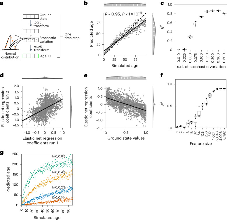
Fig. 1 Normal-distributed stochastic variation accumulation simulations enable aging clock construction for simulated data. a, Sample generation explanation with logit transform. b, Accumulating stochastic variation in logit-transformed data enables accurate simulated age predictions. The x axis shows the number of times stochastic variation was added to the ground state and the y axis shows the prediction of the independent validation data (n = 300). c, Predictions of the independent validation data are robust to the stochastic variation distribution. The x axis shows the standard deviation of the normal distribution from which the stochastic variation was sampled and the y axis shows the R2 value of the independent validation data predictions (N = 3 independent repeats; each with n = 300 independent samples). d, Coefficients of independent models are highly correlated if trained on samples starting from the same ground. Shown are the coefficients of N = 2,000 features. e, The prediction in b is possible because of a regression to the mean. The x axis shows the starting values of the 2,000 features of the simulated ground state and the y axis shows the elastic net regression coefficients for the model in b (trained on n = 300). f, The accuracy of predictions plateaus after ~2,000 features in the ground state. The x axis shows how many features were randomly sampled for the ground state and the y axis shows R2 as a measure of model accuracy (N = 10 independent repeats for features sizes <1,000, N = 3 independent repeats otherwise; each with n = 300, 3 independent samples per time point). g, The amount of stochastic variation sets the pace of aging. The elastic net regression model was trained with stochastic variation sampled from N(µ = 0, σ2 = 0.22) and tested on independent samples generated from the same ground state, but with varying degrees of stochastic variation (color-coded, as indicated in the panel). All simulated datasets consist of n = 300 independent samples. Boxplots in c and f are shown with the center line depicting the median, the box limits denote the bottom and top quartiles, and the whiskers indicate the 1.5× interquartile range.
Fig. 1 Normal-distributed stochastic variation accumulation simulations enable aging clock construction for simulated data. a, Sample generation explanation with logit transform. b, Accumulating stochastic variation in logit-transformed data enables accurate simulated age predictions. The x axis shows the number of times stochastic variation was added to the ground state and the y axis shows the prediction of the independent validation data (n = 300). c, Predictions of the independent validation data are robust to the stochastic variation distribution. The x axis shows the standard deviation of the normal distribution from which the stochastic variation was sampled and the y axis shows the R2 value of the independent validation data predictions (N = 3 independent repeats; each with n = 300 independent samples). d, Coefficients of independent models are highly correlated if trained on samples starting from the same ground. Shown are the coefficients of N = 2,000 features. e, The prediction in b is possible because of a regression to the mean. The x axis shows the starting values of the 2,000 features of the simulated ground state and the y axis shows the elastic net regression coefficients for the model in b (trained on n = 300). f, The accuracy of predictions plateaus after ~2,000 features in the ground state. The x axis shows how many features were randomly sampled for the ground state and the y axis shows R2 as a measure of model accuracy (N = 10 independent repeats for features sizes <1,000, N = 3 independent repeats otherwise; each with n = 300, 3 independent samples per time point). g, The amount of stochastic variation sets the pace of aging. The elastic net regression model was trained with stochastic variation sampled from N(µ = 0, σ2 = 0.22) and tested on independent samples generated from the same ground state, but with varying degrees of stochastic variation (color-coded, as indicated in the panel). All simulated datasets consist of n = 300 independent samples. Boxplots in c and f are shown with the center line depicting the median, the box limits denote the bottom and top quartiles, and the whiskers indicate the 1.5× interquartile range.CC BY · PubMed Central
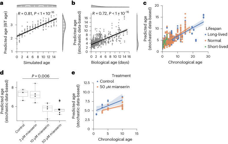
Fig. 2 Normal-distributed stochastic variation accumulation simulations enable aging clock construction for transcriptomic data. a, Simulated age and BiT age37 predictions correlate significantly (Pearson correlation: 0.81, P = 5.99 × 10−41, two-sided test); n = 160, 10 independent samples per time point. Variation was sampled with a s.d. of 0.01. b, Predictions of a transcriptomic stochastic data-based clock correlate significantly (Pearson correlation: 0.72, P = 5.7 × 10−150, two-sided test) with the biological age of n = 993 independent RNA-seq from 61 independent public datasets (Supplementary Table 1). c, There is a significant association between the median lifespan and the predicted age of the clock used in b (median lifespan coefficient P = 0.015). Regression model fit with a 95% confidence interval (shadowed area) shown for long-lived (median lifespan >20 days, blue), short-lived (median lifespan <8 days, green) and normal-lived (orange) samples. d, Mianserin shows a dose-dependent decrease in the predicted age of the clock used in b. ANOVA (P = 0.006) with a two-sided Tukeyʼs post hoc test was used (50 μM mianserin versus control adjusted P = 0.026). Boxplots are as described in Fig. 1. e, Mianserin (50 μM) shows a lower predicted age over the whole time-course (two-way ANOVA treatment P = 7.3 × 10⁻⁴). Full statistics are available in the Source Data. The regression model fit with a 95% confidence interval (shadowed area) is shown for worms receiving 50 μM mianserin (orange) and control worms (blue).
Fig. 2 Normal-distributed stochastic variation accumulation simulations enable aging clock construction for transcriptomic data. a, Simulated age and BiT age37 predictions correlate significantly (Pearson correlation: 0.81, P = 5.99 × 10−41, two-sided test); n = 160, 10 independent samples per time point. Variation was sampled with a s.d. of 0.01. b, Predictions of a transcriptomic stochastic data-based clock correlate significantly (Pearson correlation: 0.72, P = 5.7 × 10−150, two-sided test) with the biological age of n = 993 independent RNA-seq from 61 independent public datasets (Supplementary Table 1). c, There is a significant association between the median lifespan and the predicted age of the clock used in b (median lifespan coefficient P = 0.015). Regression model fit with a 95% confidence interval (shadowed area) shown for long-lived (median lifespan >20 days, blue), short-lived (median lifespan <8 days, green) and normal-lived (orange) samples. d, Mianserin shows a dose-dependent decrease in the predicted age of the clock used in b. ANOVA (P = 0.006) with a two-sided Tukeyʼs post hoc test was used (50 μM mianserin versus control adjusted P = 0.026). Boxplots are as described in Fig. 1. e, Mianserin (50 μM) shows a lower predicted age over the whole time-course (two-way ANOVA treatment P = 7.3 × 10⁻⁴). Full statistics are available in the Source Data. The regression model fit with a 95% confidence interval (shadowed area) is shown for worms receiving 50 μM mianserin (orange) and control worms (blue).CC BY · PubMed Central
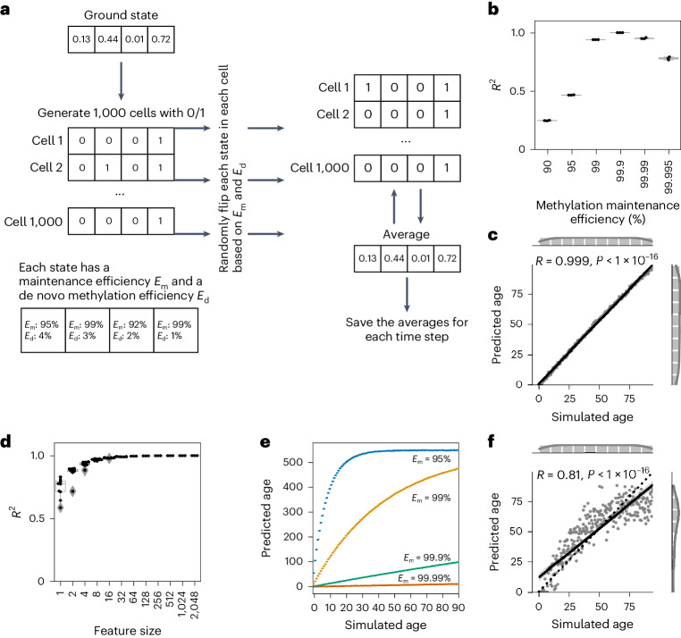
Fig. 3 Single-cell DNA methylation stochastic variation accumulation simulations enable aging clock construction for simulated data. a, Explanation of single-cell simulations. b, The accuracy of the model is dependent on the methylation maintenance efficiency rate. A stochastic data-based clock was trained with 500 features and universal maintenance efficiencies Em and Ed, and was used to predict the simulated age of 300 independent validation samples. N = 3 independent experiments with different ground states are shown for each maintenance efficiency. c, Single-cell simulation of DNA methylation sites with Em and Eu values of 99.9% allows us to build a clock with highly accurate predictions (R2 = 0.999) of independent validation data (n = 300). d, The accuracy of predictions with a universal maintenance efficiency rate of 99.9% plateaus after ~32 features with an R2 value of 0.99. N = 10 independent repeats for features sizes <1,000, N = 3 independent repeats otherwise; each with n = 300, 3 samples per time point. Boxplots in b and d are as described in Fig. 1. e, The maintenance efficiency rate sets the pace of aging. The stochastic data-based clock was trained with a maintenance efficiency of Em = Eu = 99.9%, and tested on independent samples generated from the same ground state, but with varying maintenance efficiencies (color-coded, as indicated in the panel). All simulated datasets consist of n = 300 independent samples. f, Biologically estimated maintenance rates allow for highly accurate predictions. Site-specific Em and Eu values were estimated from the data (Methods). The simulations were the same as in c but with site-specific maintenance rates (n = 300).
Fig. 3 Single-cell DNA methylation stochastic variation accumulation simulations enable aging clock construction for simulated data. a, Explanation of single-cell simulations. b, The accuracy of the model is dependent on the methylation maintenance efficiency rate. A stochastic data-based clock was trained with 500 features and universal maintenance efficiencies Em and Ed, and was used to predict the simulated age of 300 independent validation samples. N = 3 independent experiments with different ground states are shown for each maintenance efficiency. c, Single-cell simulation of DNA methylation sites with Em and Eu values of 99.9% allows us to build a clock with highly accurate predictions (R2 = 0.999) of independent validation data (n = 300). d, The accuracy of predictions with a universal maintenance efficiency rate of 99.9% plateaus after ~32 features with an R2 value of 0.99. N = 10 independent repeats for features sizes <1,000, N = 3 independent repeats otherwise; each with n = 300, 3 samples per time point. Boxplots in b and d are as described in Fig. 1. e, The maintenance efficiency rate sets the pace of aging. The stochastic data-based clock was trained with a maintenance efficiency of Em = Eu = 99.9%, and tested on independent samples generated from the same ground state, but with varying maintenance efficiencies (color-coded, as indicated in the panel). All simulated datasets consist of n = 300 independent samples. f, Biologically estimated maintenance rates allow for highly accurate predictions. Site-specific Em and Eu values were estimated from the data (Methods). The simulations were the same as in c but with site-specific maintenance rates (n = 300).CC BY · PubMed Central
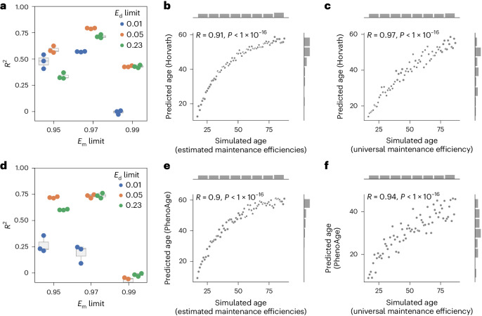
Fig. 4 Epigenetic aging clock predictions correlate significantly with the amount of stochastic variation. a, The methylation maintenance efficiency limits affect the simulation and subsequent prediction with Horvath’s epigenetic clock26. The R2 value was calculated between the predicted epigenetic age by Horvath’s epigenetic clock26 and the simulated age. N = 3 independent repeats, each consisting of n = 73 independent samples. b, Horvath’s epigenetic age prediction26 of samples simulated based on biologically estimated maintenance rates with the limits Em > 97% and Ed < 5%, correlates significantly with the simulated age. N = 73 independent samples. c, Horvath’s epigenetic age prediction26 of samples simulated based on a universal maintenance efficiency rate of 99% for all features, correlates significantly with the simulated age. N = 73 independent samples. d, Methylation maintenance efficiency limits affect the simulation and subsequent prediction with PhenoAge40. The R2 value was calculated between the predicted epigenetic age by PhenoAge40 and the simulated age. N = 3 independent repeats, each consisting of n = 73 independent samples. Boxplots in a and d are as described in Fig. 1. e, Biological age prediction with PhenoAge40 of samples simulated based on biologically estimated maintenance rates with the limits Em > 97% and Ed < 5%, correlates significantly with the simulated age. N = 73 independent samples. f, Biological age prediction with PhenoAge40 of samples simulated based on a universal maintenance rate of 99% for all features, correlates significantly with the simulated age. N = 73 independent samples.
Fig. 4 Epigenetic aging clock predictions correlate significantly with the amount of stochastic variation. a, The methylation maintenance efficiency limits affect the simulation and subsequent prediction with Horvath’s epigenetic clock26. The R2 value was calculated between the predicted epigenetic age by Horvath’s epigenetic clock26 and the simulated age. N = 3 independent repeats, each consisting of n = 73 independent samples. b, Horvath’s epigenetic age prediction26 of samples simulated based on biologically estimated maintenance rates with the limits Em > 97% and Ed < 5%, correlates significantly with the simulated age. N = 73 independent samples. c, Horvath’s epigenetic age prediction26 of samples simulated based on a universal maintenance efficiency rate of 99% for all features, correlates significantly with the simulated age. N = 73 independent samples. d, Methylation maintenance efficiency limits affect the simulation and subsequent prediction with PhenoAge40. The R2 value was calculated between the predicted epigenetic age by PhenoAge40 and the simulated age. N = 3 independent repeats, each consisting of n = 73 independent samples. Boxplots in a and d are as described in Fig. 1. e, Biological age prediction with PhenoAge40 of samples simulated based on biologically estimated maintenance rates with the limits Em > 97% and Ed < 5%, correlates significantly with the simulated age. N = 73 independent samples. f, Biological age prediction with PhenoAge40 of samples simulated based on a universal maintenance rate of 99% for all features, correlates significantly with the simulated age. N = 73 independent samples.CC BY · PubMed Central
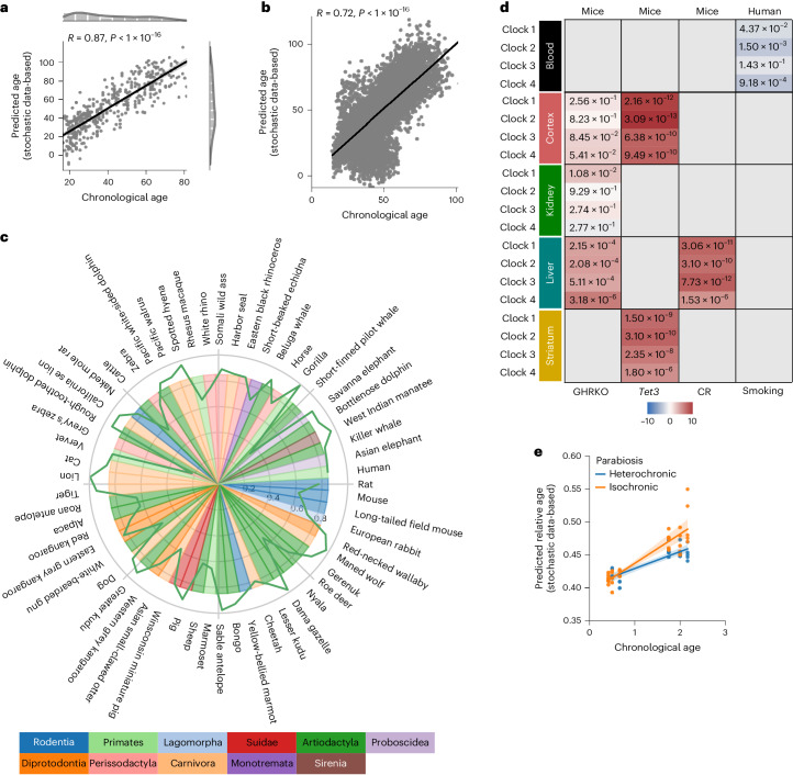
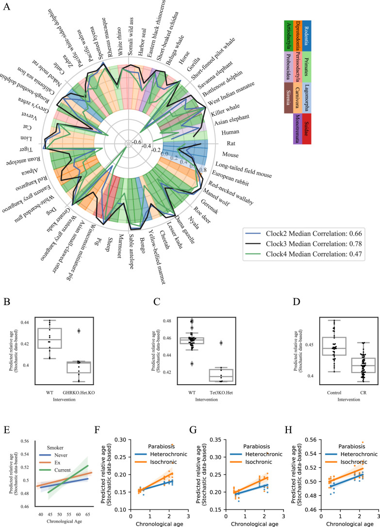
Fig. 5 Single-cell DNA methylation stochastic variation accumulation simulations enable aging clock construction for pan-mammalian chronological and biological age predictions. a, The predictions of a stochastic data-based clock correlate significantly (Pearson correlation: 0.87, P < 1 × 10⁻¹⁶, two-sided test) with the chronological age of the cell-type corrected independent healthy biological validation samples (GSE41037, n = 392)78. b, Validation of the stochastic data-based clock starting from a fetal sample (GSM4682890) on 11,146 independent samples from 15 independent datasets (GSE84727, GSE87571, GSE80417, GSE40279, GSE87648, GSE42861, GSE50660, GSE106648, GSE179325, GSE210254, GSE210255, GSE72680, GSE147740, GSE55763, GSE117860) shows a significant correlation (Pearson correlation: 0.72, P < 1 × 10⁻¹⁶, two-sided test). c, Circle plot showing the Pearson correlation between the relative age of blood samples of the corresponding species and the predictions of clock 1 as a green line around the circle. Species are shown for which at least five blood samples were available in the dataset GSE223748. The colors within the circle show the taxonomic order of the corresponding species, as listed on the left-hand side. d, Validation of Clocks 1–4 on interventions with known lifespan effects in mouse and humans. Age-matched GHRKO mice with 30 normal (12 liver, 12 kidney, 6 cerebral cortex) and 29 GHRKO (11 liver, 12 kidney, 6 cerebral cortex) samples15; Tet3-knockout mice with 28 normal (14 striatum, 14 cerebral cortex) and 16 Tet3 (8 striatum, 8 cerebral cortex) samples15; 36 CR mice with 59 normal mice15; and the effect of smoking on human aging91. The color gradient for mice is based on the sign of the t-test, the color of the human data is based on the interaction coefficient. The annotated values show the adjusted false discovery rate. e, Independent validation of clock 1 on parabiosis in young and old mice (GSE224361). Liver samples of mice that received either isochronic (orange) or heterochronic (blue) parabiosis are shown. A multivariate regression shows a significant age variable (P < 1 × 10⁻¹⁶) and interaction variable (P = 1.22 × 10⁻³). Full statistics are given in the Source Data. The regression model fit with a 95% confidence interval (shadowed area) is shown.
Fig. 5 Single-cell DNA methylation stochastic variation accumulation simulations enable aging clock construction for pan-mammalian chronological and biological age predictions. a, The predictions of a stochastic data-based clock correlate significantly (Pearson correlation: 0.87, P < 1 × 10⁻¹⁶, two-sided test) with the chronological age of the cell-type corrected independent healthy biological validation samples (GSE41037, n = 392)78. b, Validation of the stochastic data-based clock starting from a fetal sample (GSM4682890) on 11,146 independent samples from 15 independent datasets (GSE84727, GSE87571, GSE80417, GSE40279, GSE87648, GSE42861, GSE50660, GSE106648, GSE179325, GSE210254, GSE210255, GSE72680, GSE147740, GSE55763, GSE117860) shows a significant correlation (Pearson correlation: 0.72, P < 1 × 10⁻¹⁶, two-sided test). c, Circle plot showing the Pearson correlation between the relative age of blood samples of the corresponding species and the predictions of clock 1 as a green line around the circle. Species are shown for which at least five blood samples were available in the dataset GSE223748. The colors within the circle show the taxonomic order of the corresponding species, as listed on the left-hand side. d, Validation of Clocks 1–4 on interventions with known lifespan effects in mouse and humans. Age-matched GHRKO mice with 30 normal (12 liver, 12 kidney, 6 cerebral cortex) and 29 GHRKO (11 liver, 12 kidney, 6 cerebral cortex) samples15; Tet3-knockout mice with 28 normal (14 striatum, 14 cerebral cortex) and 16 Tet3 (8 striatum, 8 cerebral cortex) samples15; 36 CR mice with 59 normal mice15; and the effect of smoking on human aging91. The color gradient for mice is based on the sign of the t-test, the color of the human data is based on the interaction coefficient. The annotated values show the adjusted false discovery rate. e, Independent validation of clock 1 on parabiosis in young and old mice (GSE224361). Liver samples of mice that received either isochronic (orange) or heterochronic (blue) parabiosis are shown. A multivariate regression shows a significant age variable (P < 1 × 10⁻¹⁶) and interaction variable (P = 1.22 × 10⁻³). Full statistics are given in the Source Data. The regression model fit with a 95% confidence interval (shadowed area) is shown.CC BY · PubMed Central
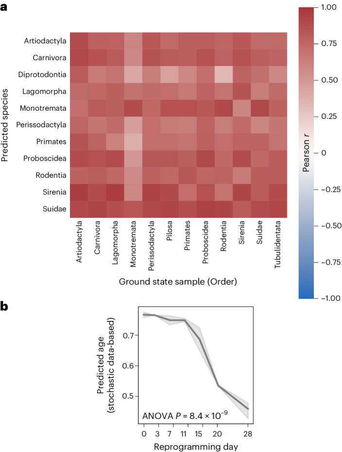
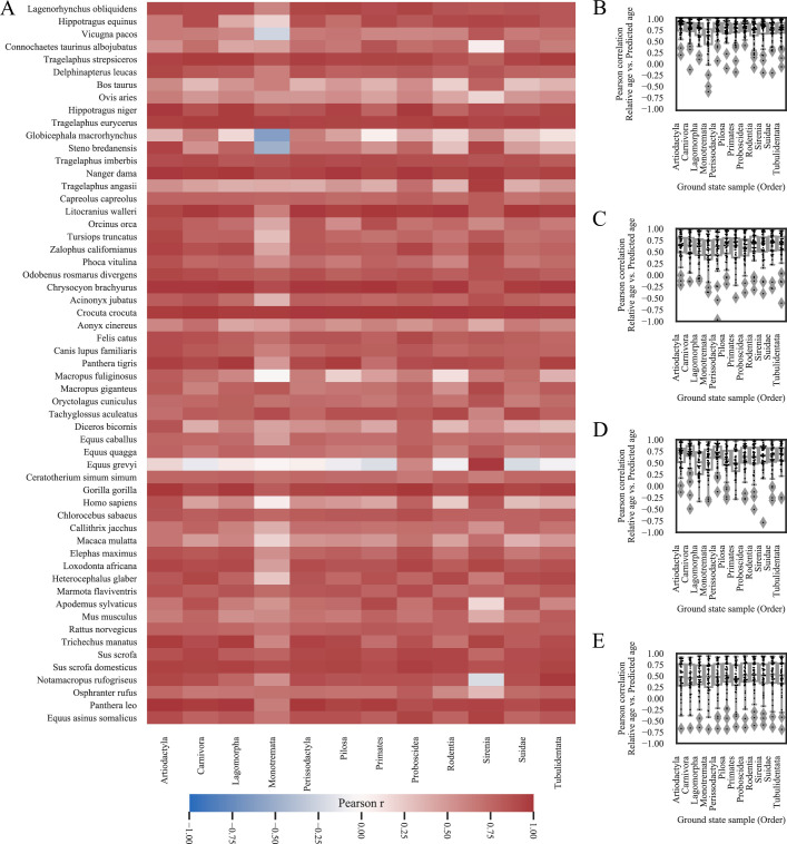
Fig. 6 Single-cell DNA methylation stochastic variation accumulation simulations enable predictions for various species and reprogramming. a, Heatmap showing median Pearson correlations of species in the same taxonomic order between the predicted age of clock 1 trained on the youngest blood sample from species of the corresponding taxonomic order in the columns (Artiodactyla: Tursiops truncatus; Carnivora: Odobenus rosmarus divergens; Lagomorpha: Oryctolagus cuniculus; Monotremata: Tachyglossus aculeatus; Perissodactyla: Equus caballus; Pilosa: Choloepus hoffmanni; Proboscidea: Loxodonta africana; Rodentia: Marmota flaviventris; Sirenia: Trichechus manatus; Suidae: Sus scrofa; Tubulidentata: Orycteropus afer) and the relative age for all species in the rows. Values are shown for tissues and species for which at least five samples were available. b, The stochastic data-based clock in Fig. 5c was used on an independent reprogramming time-course dataset of human dermal fibroblasts (GSE54848)49. One-way ANOVA, P = 8.36 × 10⁻⁹ (statistics are shown in the Source Data). The line plot shows the mean values with a 95% confidence interval (shadowed area).
Fig. 6 Single-cell DNA methylation stochastic variation accumulation simulations enable predictions for various species and reprogramming. a, Heatmap showing median Pearson correlations of species in the same taxonomic order between the predicted age of clock 1 trained on the youngest blood sample from species of the corresponding taxonomic order in the columns (Artiodactyla: Tursiops truncatus; Carnivora: Odobenus rosmarus divergens; Lagomorpha: Oryctolagus cuniculus; Monotremata: Tachyglossus aculeatus; Perissodactyla: Equus caballus; Pilosa: Choloepus hoffmanni; Proboscidea: Loxodonta africana; Rodentia: Marmota flaviventris; Sirenia: Trichechus manatus; Suidae: Sus scrofa; Tubulidentata: Orycteropus afer) and the relative age for all species in the rows. Values are shown for tissues and species for which at least five samples were available. b, The stochastic data-based clock in Fig. 5c was used on an independent reprogramming time-course dataset of human dermal fibroblasts (GSE54848)49. One-way ANOVA, P = 8.36 × 10⁻⁹ (statistics are shown in the Source Data). The line plot shows the mean values with a 95% confidence interval (shadowed area).CC BY · PubMed Central
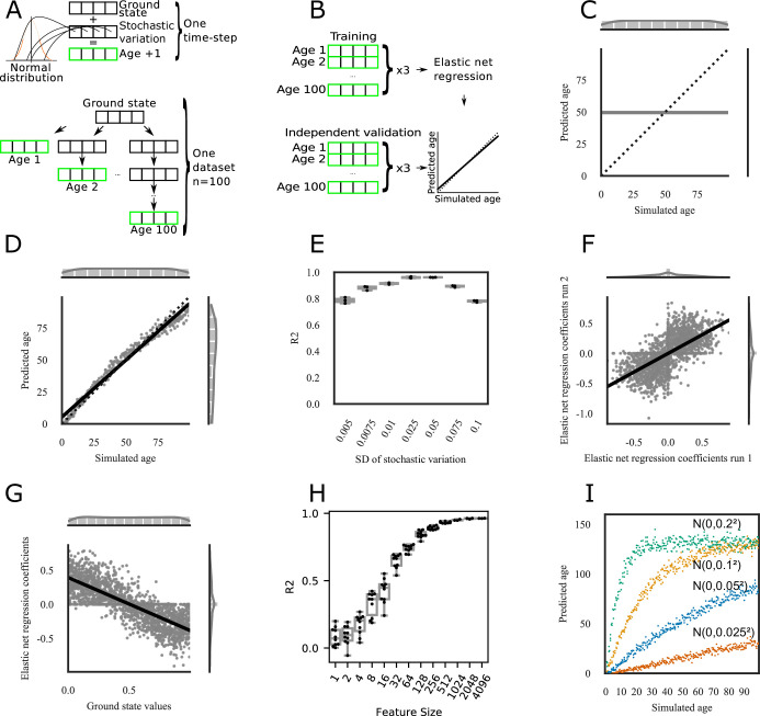
Extended Data Fig. 1 Normal-distributed stochastic variation accumulation simulations with value limits enable aging clock construction for simulated data. a) Sample generation explanation. One time-step is defined as the addition of one-time stochastic variation, that is random noise, to each feature of the ground state that is sampled from a normal distribution centered at 0 (Top). Samples with different simulated ages are generated starting from the same ground state, but independently from each other (Bottom). A sample of age 1 adds normal-distributed stochastic variation once to the ground state, a sample of age 2 twice independently, and so on. b) Model training and validation explanation. For training and validation 3 sets of independent samples are generated from the same ground state as explained in Extended Data Fig. 1a. 3 sets comprising the whole age-range, for example 1–100, are used as an input for an Elastic net regression to train a predictor that predicts the simulated age of a sample, that is how often stochastic variation was added to the ground state. The 3 independent datasets are used to validate the model and assess the accuracy. c) Unlimited stochastic variation does not allow for any prediction. All samples within the training and validation dataset started from the same ground state of 2000 uniformly randomly sampled features between 0 and 1. For every whole simulated age step from 1 to 100, normal-distributed stochastic variation sampled from N(µ = 0, σ2 = 0.052) was added. n = 300 samples (3 independent samples per age step) were used for training of the Elastic net regression model to predict the simulated age, and n = 300 independent samples were used for validation. The x-axis shows the true simulated age, that is the number of times random stochastic variation was added to the ground state. The y-axis shows the prediction of the Elastic net regression model of the independent validation data (n = 300, 3 independent samples per time point). The sides show the distribution of the samples. d) Same as C), but after addition of stochastic variation the values were kept within the range of 0–1, for example values bigger to 1 were set to 1 (n = 300, 3 independent samples per time point). Limiting the values after stochastic variation application allows to build highly accurate predictors of the simulated age. e) The predictions of the independent validation data are robust to the stochastic variation distribution. The samples were simulated the same as in D) with different stochastic variation distributions (n = 300, 3 independent samples per time point). The x-axis shows the standard deviation of the normal distribution from which the stochastic variation was sampled, that is N(µ = 0, σ2 = 0.0052) has a narrow noise distribution with 99.7 % of the sampled data within the range [−0.015, 0.015], while N(µ = 0, σ2 = 0.012) has a wide distribution with 99.7 % of the sampled data within the range [-0.3, 0.3]. The y-axis shows the R² value between the simulated age and the predicted age of the independent validation data (N = 3 independent repeats; each with n = 300, 3 samples per time point). Boxplots are shown with the center line depicting the median, the box limits the bottom, respective top quartiles, and the whiskers the 1.5x interquartile range. f) Independent Elastic net regression models are highly correlated if trained on samples starting from the same ground state (consisting of N = 2000 uniformly randomly sampled features between 0 and 1). The x-axis shows the coefficients of the Elastic net regression of D), and the y-axis shows the coefficients of an independent Elastic net regression on samples that started with the same ground state, but with independent stochastic variation application (trained on n = 300, 3 samples per time point). g) The prediction in D) is possible due to a regression to the mean. The x-axis shows the starting values of the 2000 features of the simulated ground state, the y-axis the Elastic net regression coefficients for the model in D) (trained on n = 300, 3 samples per time point). Features starting close to 0 have a positive coefficient, indicating an increase over the simulated time period, while features close to 1 have a negative coefficient, indicating a decrease. Features close to 0.5 are more sensitive to random changes and are closer to 0. h) The accuracy of predictions caps off after ~1000 features in the ground state. The x-axis shows how many uniformly randomly features were sampled for the ground state that was used to build and validate an Elastic net regression model the same as in D) (trained on n = 300, 3 samples per time point). The y-axis shows the R² as a measure of model accuracy. Of note, the Elastic net regression will shrink coefficients of features to 0 and thereby reduce the features relevant for the prediction further. (N = 10 independent repeats for Features Sizes<1000, N = 3 independent repeats otherwise; each with n = 300, 3 samples per time point). Boxplots are shown with the center line depicting the median, the box limits the bottom, respective top quartiles, and the whiskers the 1.5x interquartile range. i) The amount of stochastic variation sets the pace of aging. The Elastic net regression model was trained the same as in D) with stochastic variation sampled from N(µ = 0, σ2 = 0.052) (n = 300, 3 samples per time point). Color-coded are different independent validation samples, generated from the same ground state, but with stochastic variation from different normal distributions. Samples with stochastic variation from a distribution with a narrower standard deviation (N(µ = 0, σ2 = 0.0252)) accumulate less noise and are predicted to age slower, that is the slope of the prediction is lower. Samples with stochastic variation from a distribution with a wider standard deviation (N(µ = 0, σ2 = 0.12), N(µ = 0, σ2 = 0.22)) accumulate noise faster, have a steeper slope of prediction, and reach the maximum age faster. The x-axis shows the true simulated age, that is the number of times stochastic variation was added to the ground state. The y-axis shows the prediction of the Elastic net regression model of the independent validation data. All 4 simulated datasets consist of n = 300, 3 samples per time point.
Extended Data Fig. 1 Normal-distributed stochastic variation accumulation simulations with value limits enable aging clock construction for simulated data. a) Sample generation explanation. One time-step is defined as the addition of one-time stochastic variation, that is random noise, to each feature of the ground state that is sampled from a normal distribution centered at 0 (Top). Samples with different simulated ages are generated starting from the same ground state, but independently from each other (Bottom). A sample of age 1 adds normal-distributed stochastic variation once to the ground state, a sample of age 2 twice independently, and so on. b) Model training and validation explanation. For training and validation 3 sets of independent samples are generated from the same ground state as explained in Extended Data Fig. 1a. 3 sets comprising the whole age-range, for example 1–100, are used as an input for an Elastic net regression to train a predictor that predicts the simulated age of a sample, that is how often stochastic variation was added to the ground state. The 3 independent datasets are used to validate the model and assess the accuracy. c) Unlimited stochastic variation does not allow for any prediction. All samples within the training and validation dataset started from the same ground state of 2000 uniformly randomly sampled features between 0 and 1. For every whole simulated age step from 1 to 100, normal-distributed stochastic variation sampled from N(µ = 0, σ2 = 0.052) was added. n = 300 samples (3 independent samples per age step) were used for training of the Elastic net regression model to predict the simulated age, and n = 300 independent samples were used for validation. The x-axis shows the true simulated age, that is the number of times random stochastic variation was added to the ground state. The y-axis shows the prediction of the Elastic net regression model of the independent validation data (n = 300, 3 independent samples per time point). The sides show the distribution of the samples. d) Same as C), but after addition of stochastic variation the values were kept within the range of 0–1, for example values bigger to 1 were set to 1 (n = 300, 3 independent samples per time point). Limiting the values after stochastic variation application allows to build highly accurate predictors of the simulated age. e) The predictions of the independent validation data are robust to the stochastic variation distribution. The samples were simulated the same as in D) with different stochastic variation distributions (n = 300, 3 independent samples per time point). The x-axis shows the standard deviation of the normal distribution from which the stochastic variation was sampled, that is N(µ = 0, σ2 = 0.0052) has a narrow noise distribution with 99.7 % of the sampled data within the range [−0.015, 0.015], while N(µ = 0, σ2 = 0.012) has a wide distribution with 99.7 % of the sampled data within the range [-0.3, 0.3]. The y-axis shows the R² value between the simulated age and the predicted age of the independent validation data (N = 3 independent repeats; each with n = 300, 3 samples per time point). Boxplots are shown with the center line depicting the median, the box limits the bottom, respective top quartiles, and the whiskers the 1.5x interquartile range. f) Independent Elastic net regression models are highly correlated if trained on samples starting from the same ground state (consisting of N = 2000 uniformly randomly sampled features between 0 and 1). The x-axis shows the coefficients of the Elastic net regression of D), and the y-axis shows the coefficients of an independent Elastic net regression on samples that started with the same ground state, but with independent stochastic variation application (trained on n = 300, 3 samples per time point). g) The prediction in D) is possible due to a regression to the mean. The x-axis shows the starting values of the 2000 features of the simulated ground state, the y-axis the Elastic net regression coefficients for the model in D) (trained on n = 300, 3 samples per time point). Features starting close to 0 have a positive coefficient, indicating an increase over the simulated time period, while features close to 1 have a negative coefficient, indicating a decrease. Features close to 0.5 are more sensitive to random changes and are closer to 0. h) The accuracy of predictions caps off after ~1000 features in the ground state. The x-axis shows how many uniformly randomly features were sampled for the ground state that was used to build and validate an Elastic net regression model the same as in D) (trained on n = 300, 3 samples per time point). The y-axis shows the R² as a measure of model accuracy. Of note, the Elastic net regression will shrink coefficients of features to 0 and thereby reduce the features relevant for the prediction further. (N = 10 independent repeats for Features Sizes<1000, N = 3 independent repeats otherwise; each with n = 300, 3 samples per time point). Boxplots are shown with the center line depicting the median, the box limits the bottom, respective top quartiles, and the whiskers the 1.5x interquartile range. i) The amount of stochastic variation sets the pace of aging. The Elastic net regression model was trained the same as in D) with stochastic variation sampled from N(µ = 0, σ2 = 0.052) (n = 300, 3 samples per time point). Color-coded are different independent validation samples, generated from the same ground state, but with stochastic variation from different normal distributions. Samples with stochastic variation from a distribution with a narrower standard deviation (N(µ = 0, σ2 = 0.0252)) accumulate less noise and are predicted to age slower, that is the slope of the prediction is lower. Samples with stochastic variation from a distribution with a wider standard deviation (N(µ = 0, σ2 = 0.12), N(µ = 0, σ2 = 0.22)) accumulate noise faster, have a steeper slope of prediction, and reach the maximum age faster. The x-axis shows the true simulated age, that is the number of times stochastic variation was added to the ground state. The y-axis shows the prediction of the Elastic net regression model of the independent validation data. All 4 simulated datasets consist of n = 300, 3 samples per time point.CC BY · PubMed Central
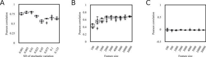
Extended Data Fig. 2 The effect of the feature size and the amount of stochastic variation on transcriptomic stochastic variation accumulation simulations. a) The BitAge predictions in Fig. 2a are robust to the distribution from which the stochastic variation is sampled. The x-axis shows the standard deviation of the normal distribution (centered at 0) from which stochastic variation for the simulations is sampled. The y-axis shows the Pearson correlation between the BitAge prediction of the simulated samples and the number of stochastic variation additions of the samples. Stochastic variation sampled from a normal distribution centered at 0 and a standard variation of 0.01 shows the highest Pearson correlation. N = 5 independent experiments are shown. Boxplots are shown with the center line depicting the median, the box limits the bottom, respective top quartiles, and the whiskers the 1.5x interquartile range. b) The feature size is largely irrelevant for the model in Fig. 2b). Predictions of Elastic net regression models trained on more than 100 features are significantly correlated with the biological age of C. elegans samples. The x-axis shows the number of randomly selected features, that is genes, for the ground state, which were subsequently used to generate data based on stochastic variations (see methods for details). These simulated samples were used to train the Elastic net regression. The y-axis shows the Pearson correlation between the biological age of the 993 independent samples (excluding the sample from which the ground state was sampled) and the prediction of the independent stochastic-data based model. N = 10 independent experiments are shown. Boxplots are shown with the center line depicting the median, the box limits the bottom, respective top quartiles, and the whiskers the 1.5x interquartile range. c) Verification of Extended Data Fig. 2b). Using the same approach as in Extended Data Fig. 2b, but with randomly shuffled biological ages of the C. elegans samples shows no significant correlation, indicating that biological age, and not a confounding variable is correlated with the predictions of the model based on simulated data. The x-axis shows the number of randomly selected features, that is genes, for the ground state, which were subsequently used to generate data based on stochastic variations (see methods for details. These simulated samples were used to train the Elastic net regression. The y-axis shows the Pearson correlation between the biological age of the 993 independent samples (excluding the sample from which the ground state was sampled) and the prediction of the stochastic-data based model. N = 10 independent experiments are shown. Boxplots are shown with the center line depicting the median, the box limits the bottom, respective top quartiles, and the whiskers the 1.5x interquartile range.
Extended Data Fig. 2 The effect of the feature size and the amount of stochastic variation on transcriptomic stochastic variation accumulation simulations. a) The BitAge predictions in Fig. 2a are robust to the distribution from which the stochastic variation is sampled. The x-axis shows the standard deviation of the normal distribution (centered at 0) from which stochastic variation for the simulations is sampled. The y-axis shows the Pearson correlation between the BitAge prediction of the simulated samples and the number of stochastic variation additions of the samples. Stochastic variation sampled from a normal distribution centered at 0 and a standard variation of 0.01 shows the highest Pearson correlation. N = 5 independent experiments are shown. Boxplots are shown with the center line depicting the median, the box limits the bottom, respective top quartiles, and the whiskers the 1.5x interquartile range. b) The feature size is largely irrelevant for the model in Fig. 2b). Predictions of Elastic net regression models trained on more than 100 features are significantly correlated with the biological age of C. elegans samples. The x-axis shows the number of randomly selected features, that is genes, for the ground state, which were subsequently used to generate data based on stochastic variations (see methods for details). These simulated samples were used to train the Elastic net regression. The y-axis shows the Pearson correlation between the biological age of the 993 independent samples (excluding the sample from which the ground state was sampled) and the prediction of the independent stochastic-data based model. N = 10 independent experiments are shown. Boxplots are shown with the center line depicting the median, the box limits the bottom, respective top quartiles, and the whiskers the 1.5x interquartile range. c) Verification of Extended Data Fig. 2b). Using the same approach as in Extended Data Fig. 2b, but with randomly shuffled biological ages of the C. elegans samples shows no significant correlation, indicating that biological age, and not a confounding variable is correlated with the predictions of the model based on simulated data. The x-axis shows the number of randomly selected features, that is genes, for the ground state, which were subsequently used to generate data based on stochastic variations (see methods for details. These simulated samples were used to train the Elastic net regression. The y-axis shows the Pearson correlation between the biological age of the 993 independent samples (excluding the sample from which the ground state was sampled) and the prediction of the stochastic-data based model. N = 10 independent experiments are shown. Boxplots are shown with the center line depicting the median, the box limits the bottom, respective top quartiles, and the whiskers the 1.5x interquartile range.CC BY · PubMed Central
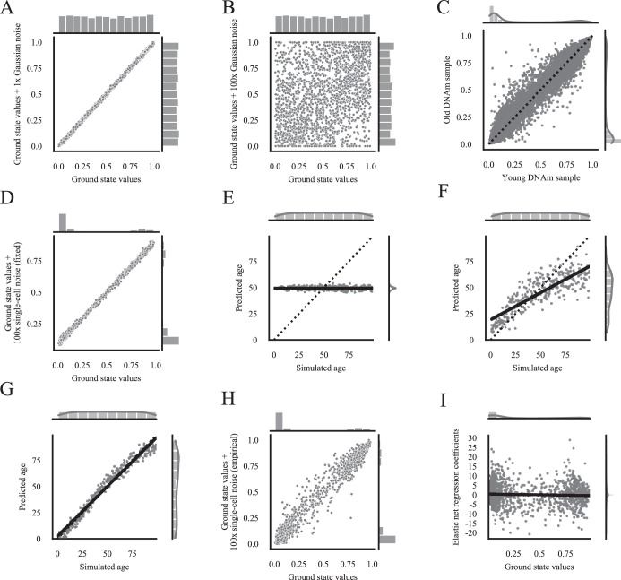
Extended Data Fig. 3 DNA methylation stochastic variation accumulation simulations. a) Comparison between the ground state on the x-axis, and the ground state (N = 2000 uniformly randomly sampled features between 0 and 1) after applying stochastic variation from N(µ = 0, σ2 = 0.052), that is Gaussian noise, once on the y-axis. b) Comparison between the ground state on the x-axis, and the ground state (N = 2000 uniformly randomly sampled features between 0 and 1) after applying stochastic variation from N(µ = 0, σ2 = 0.052), that is Gaussian noise, 100 times on the y-axis. c) Comparison of human blood DNA methylation data of the youngest (x-axis= GSM1007467) and oldest (y-axis= GSM1007832) subjects in the public dataset GSE41037 ref. 78. Every dot depicts a DNA methylation site (n = 21389). Values close to 0 and 1 show less variation than values closer to 0.5. d) Comparison of the ground state on the x-axis (2000 randomly sampled features from the youngest healthy sample (GSM1007467 ref. 78)) and the ground state after applying 100x single cell stochastic variation steps with a universal maintenance efficiency rate of 99.9 %, that is the maintenance efficiency rate is fixed to be the same for all features (y-axis). e) Starting single-cell simulations with a ground state consisting of 2000 features at 0.5 with a universal maintenance of 99 % allows no prediction. An Elastic net regression model was trained on n = 300 samples (3 samples per time point) starting from the same ground state in which all features were set to 0.5, and universal maintenance efficiencies Em and Eu of 99 %. The x-axis shows the true simulated age, that is the number of times stochastic variation was added to the ground state. The y-axis shows the prediction of the Elastic net regression model of the independent validation data (n = 300, 3 samples per time point). The sides show the distribution of the samples. f) Starting single-cell simulations with a ground state consisting of 2000 features at 0.51 with a universal maintenance of 99 % allows for an accurate age prediction. The training and validation were done the same as in B) with the difference that all features in the ground state started at 0.51. (n = 300, 3 samples per time point). g) Starting single-cell simulations with a ground state consisting of 2000 features at 0.5 with biologically estimated maintenance rates allows for an accurate prediction. The training and validation were done the same as in B) with the difference that Em and Eu values were estimated from biological data (see methods for details). (n = 300, 3 samples per time point). h) Comparison of the ground state on the x-axis (2000 randomly sampled features from the youngest healthy sample (GSM1007467 ref. 78)) and the ground state after applying 100x single cell stochastic variation steps (y-axis) with empirically estimated maintenance efficiency rates with the limits Em > 95 % and Ed < 23 %. i) The prediction in Fig. 3f) is not due to a regression to the mean, different to Fig. 1. The x-axis shows the starting values of the 2000 randomly sampled features from the youngest healthy sample (GSM1007467 ref. 78) as the ground state, the y-axis the Elastic net regression coefficients for the model in Fig. 3f) (n = 300, 3 samples per time point). All ground state features can have positive as well as negative coefficients, indicating that the prediction is not based on a regression to the mean.
Extended Data Fig. 3 DNA methylation stochastic variation accumulation simulations. a) Comparison between the ground state on the x-axis, and the ground state (N = 2000 uniformly randomly sampled features between 0 and 1) after applying stochastic variation from N(µ = 0, σ2 = 0.052), that is Gaussian noise, once on the y-axis. b) Comparison between the ground state on the x-axis, and the ground state (N = 2000 uniformly randomly sampled features between 0 and 1) after applying stochastic variation from N(µ = 0, σ2 = 0.052), that is Gaussian noise, 100 times on the y-axis. c) Comparison of human blood DNA methylation data of the youngest (x-axis= GSM1007467) and oldest (y-axis= GSM1007832) subjects in the public dataset GSE41037 ref. 78. Every dot depicts a DNA methylation site (n = 21389). Values close to 0 and 1 show less variation than values closer to 0.5. d) Comparison of the ground state on the x-axis (2000 randomly sampled features from the youngest healthy sample (GSM1007467 ref. 78)) and the ground state after applying 100x single cell stochastic variation steps with a universal maintenance efficiency rate of 99.9 %, that is the maintenance efficiency rate is fixed to be the same for all features (y-axis). e) Starting single-cell simulations with a ground state consisting of 2000 features at 0.5 with a universal maintenance of 99 % allows no prediction. An Elastic net regression model was trained on n = 300 samples (3 samples per time point) starting from the same ground state in which all features were set to 0.5, and universal maintenance efficiencies Em and Eu of 99 %. The x-axis shows the true simulated age, that is the number of times stochastic variation was added to the ground state. The y-axis shows the prediction of the Elastic net regression model of the independent validation data (n = 300, 3 samples per time point). The sides show the distribution of the samples. f) Starting single-cell simulations with a ground state consisting of 2000 features at 0.51 with a universal maintenance of 99 % allows for an accurate age prediction. The training and validation were done the same as in B) with the difference that all features in the ground state started at 0.51. (n = 300, 3 samples per time point). g) Starting single-cell simulations with a ground state consisting of 2000 features at 0.5 with biologically estimated maintenance rates allows for an accurate prediction. The training and validation were done the same as in B) with the difference that Em and Eu values were estimated from biological data (see methods for details). (n = 300, 3 samples per time point). h) Comparison of the ground state on the x-axis (2000 randomly sampled features from the youngest healthy sample (GSM1007467 ref. 78)) and the ground state after applying 100x single cell stochastic variation steps (y-axis) with empirically estimated maintenance efficiency rates with the limits Em > 95 % and Ed < 23 %. i) The prediction in Fig. 3f) is not due to a regression to the mean, different to Fig. 1. The x-axis shows the starting values of the 2000 randomly sampled features from the youngest healthy sample (GSM1007467 ref. 78) as the ground state, the y-axis the Elastic net regression coefficients for the model in Fig. 3f) (n = 300, 3 samples per time point). All ground state features can have positive as well as negative coefficients, indicating that the prediction is not based on a regression to the mean.CC BY · PubMed Central
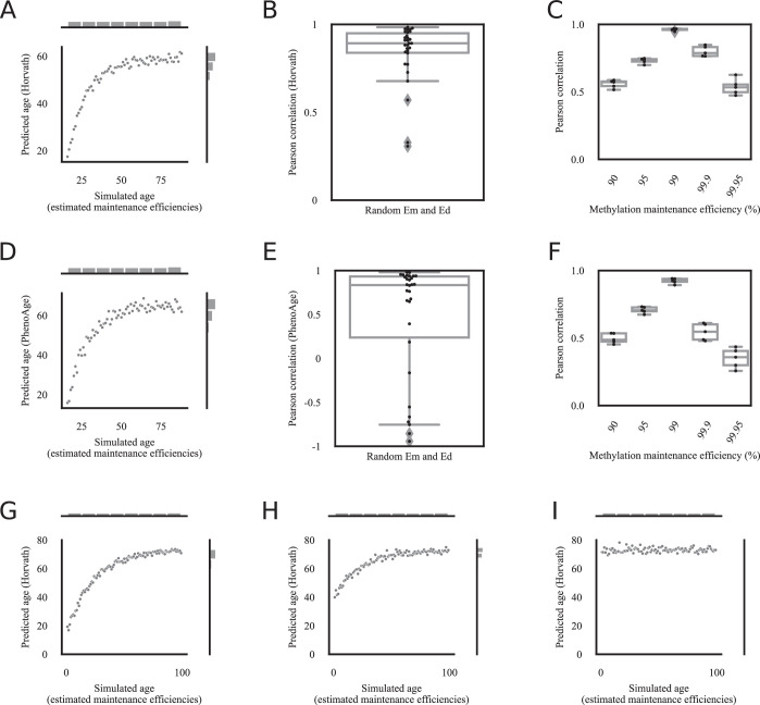
Extended Data Fig. 4 Epigenetic aging clock predictions correlate robustly with the amount of stochastic variation. a) Horvath’s epigenetic age prediction26 of samples simulated based on biologically estimated maintenance rates with the limits Em > 95 % and Ed < 23 % starting from biological data from a young human blood sample (GSM1007467)78, correlates significantly with the simulated age, that is how often stochastic variation was applied to the ground state. N = 73 independent samples, one per age step from 16 to 88 are shown. b) Horvath’s epigenetic age prediction26 of samples simulated based on random maintenance rates within the limits 97%<Em≤100% and 0%≤Ed<5% starting from biological data from a young human blood sample (GSM1007467)78, correlates significantly with the simulated age, that is how often stochastic variation was applied to the ground state. The y-axis shows the Pearson correlation between the simulated age and Horvath’s age prediction. N = 30 independent experiments with each n = 73 independent samples. Boxplots are shown with the center line depicting the median, the box limits the bottom, respective top quartiles, and the whiskers the 1.5x interquartile range. c) Pearson correlation of Horvath’s epigenetic age prediction26 of simulated data and the true simulated age for different universal methylation maintenance efficiencies. 5 independent experiments (each containing n = 73 independent samples, one per age step from 16 to 88) with different ground states are shown for each maintenance efficiency. Boxplots are shown with the center line depicting the median, the box limits the bottom, respective top quartiles, and the whiskers the 1.5x interquartile range. d) Biological age prediction with PhenoAge40 of samples simulated based on biologically estimated maintenance rates with the limits Em > 95 % and Ed < 23 % starting from biological data from a young human blood sample (GSM1007467)78, correlates significantly with the simulated age, that is how often stochastic variation was applied to the ground state. N = 73 independent samples, one per age step from 16 to 88 are shown. e) Biological age prediction with PhenoAge40 of samples simulated based on random maintenance rates within the limits 97%<Em≤100% and 0%≤Ed<5% starting from biological data from a young human blood sample (GSM1007467)78, correlates significantly with the simulated age, that is how often stochastic variation was applied to the ground state. The y-axis shows the Pearson correlation between the simulated age and PhenoAge’s age prediction. N = 30 independent experiments with each n = 73 independent samples. The boxplot is shown with the center line depicting the median, the box limits the bottom, respective top quartiles, and the whiskers the 1.5x interquartile range. f) Pearson correlation of biological age predictions with PhenoAge40 of simulated data and the true simulated age for different universal methylation maintenance efficiencies. 5 independent experiments (each containing n = 73 independent samples, one per age step from 16 to 88) with different ground states are shown for each maintenance efficiency. Boxplots are shown with the center line depicting the median, the box limits the bottom, respective top quartiles, and the whiskers the 1.5x interquartile range. g) Horvath’s epigenetic age prediction26 of samples simulated based on biologically estimated maintenance rates with the limits Em > 97 % and Ed < 5 % starting from biological data from a young human blood sample age 16 (GSM1007467)78, correlates significantly with the simulated age, that is how often stochastic variation was applied to the ground state. The simulation is the same as in Extended Data Fig. 4a, but with a simulated age range from 0–99 for an easier comparison with Extended Data Fig. 4h, i. N = 100 independent samples, one per age step from 0 to 99 are shown. h) Horvath’s epigenetic age prediction26 of samples simulated based on biologically estimated maintenance rates with the limits Em > 97 % and Ed < 5 % starting from biological data from a middle-aged human blood sample age 37 (GSM1007384)78, still correlates significantly with the simulated age, that is how often stochastic variation was applied to the ground state. The predicted age starts at a later time-point than the predictions in Extended Data Fig. 4g, and reaches the cap-off earlier. N = 100 independent samples, one per age step from 0 to 99 are shown. i) Horvath’s epigenetic age prediction26 of samples simulated based on biologically estimated maintenance rates with the limits Em > 97 % and Ed < 5 % starting from biological data from an old human blood sample age 81 (GSM1007791)78, does not correlate significantly with the simulated age, that is how often stochastic variation was applied to the ground state. Starting the ground state at an old age does not allow for a correlation between the predicted epigenetic age and the amount of stochastic variation in the data, since the prediction already starts in the cap-off. N = 100 independent samples, one per age step from 0 to 99 are shown.
Extended Data Fig. 4 Epigenetic aging clock predictions correlate robustly with the amount of stochastic variation. a) Horvath’s epigenetic age prediction26 of samples simulated based on biologically estimated maintenance rates with the limits Em > 95 % and Ed < 23 % starting from biological data from a young human blood sample (GSM1007467)78, correlates significantly with the simulated age, that is how often stochastic variation was applied to the ground state. N = 73 independent samples, one per age step from 16 to 88 are shown. b) Horvath’s epigenetic age prediction26 of samples simulated based on random maintenance rates within the limits 97%<Em≤100% and 0%≤Ed<5% starting from biological data from a young human blood sample (GSM1007467)78, correlates significantly with the simulated age, that is how often stochastic variation was applied to the ground state. The y-axis shows the Pearson correlation between the simulated age and Horvath’s age prediction. N = 30 independent experiments with each n = 73 independent samples. Boxplots are shown with the center line depicting the median, the box limits the bottom, respective top quartiles, and the whiskers the 1.5x interquartile range. c) Pearson correlation of Horvath’s epigenetic age prediction26 of simulated data and the true simulated age for different universal methylation maintenance efficiencies. 5 independent experiments (each containing n = 73 independent samples, one per age step from 16 to 88) with different ground states are shown for each maintenance efficiency. Boxplots are shown with the center line depicting the median, the box limits the bottom, respective top quartiles, and the whiskers the 1.5x interquartile range. d) Biological age prediction with PhenoAge40 of samples simulated based on biologically estimated maintenance rates with the limits Em > 95 % and Ed < 23 % starting from biological data from a young human blood sample (GSM1007467)78, correlates significantly with the simulated age, that is how often stochastic variation was applied to the ground state. N = 73 independent samples, one per age step from 16 to 88 are shown. e) Biological age prediction with PhenoAge40 of samples simulated based on random maintenance rates within the limits 97%<Em≤100% and 0%≤Ed<5% starting from biological data from a young human blood sample (GSM1007467)78, correlates significantly with the simulated age, that is how often stochastic variation was applied to the ground state. The y-axis shows the Pearson correlation between the simulated age and PhenoAge’s age prediction. N = 30 independent experiments with each n = 73 independent samples. The boxplot is shown with the center line depicting the median, the box limits the bottom, respective top quartiles, and the whiskers the 1.5x interquartile range. f) Pearson correlation of biological age predictions with PhenoAge40 of simulated data and the true simulated age for different universal methylation maintenance efficiencies. 5 independent experiments (each containing n = 73 independent samples, one per age step from 16 to 88) with different ground states are shown for each maintenance efficiency. Boxplots are shown with the center line depicting the median, the box limits the bottom, respective top quartiles, and the whiskers the 1.5x interquartile range. g) Horvath’s epigenetic age prediction26 of samples simulated based on biologically estimated maintenance rates with the limits Em > 97 % and Ed < 5 % starting from biological data from a young human blood sample age 16 (GSM1007467)78, correlates significantly with the simulated age, that is how often stochastic variation was applied to the ground state. The simulation is the same as in Extended Data Fig. 4a, but with a simulated age range from 0–99 for an easier comparison with Extended Data Fig. 4h, i. N = 100 independent samples, one per age step from 0 to 99 are shown. h) Horvath’s epigenetic age prediction26 of samples simulated based on biologically estimated maintenance rates with the limits Em > 97 % and Ed < 5 % starting from biological data from a middle-aged human blood sample age 37 (GSM1007384)78, still correlates significantly with the simulated age, that is how often stochastic variation was applied to the ground state. The predicted age starts at a later time-point than the predictions in Extended Data Fig. 4g, and reaches the cap-off earlier. N = 100 independent samples, one per age step from 0 to 99 are shown. i) Horvath’s epigenetic age prediction26 of samples simulated based on biologically estimated maintenance rates with the limits Em > 97 % and Ed < 5 % starting from biological data from an old human blood sample age 81 (GSM1007791)78, does not correlate significantly with the simulated age, that is how often stochastic variation was applied to the ground state. Starting the ground state at an old age does not allow for a correlation between the predicted epigenetic age and the amount of stochastic variation in the data, since the prediction already starts in the cap-off. N = 100 independent samples, one per age step from 0 to 99 are shown.CC BY · PubMed Central
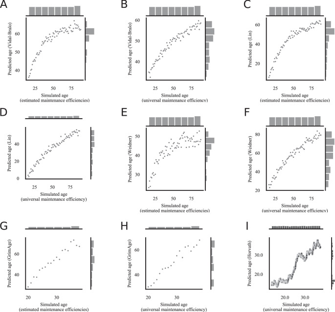
Extended Data Fig. 5 All tested epigenetic clock predictions correlate significantly with the amount of stochastic variation. a) Vidal-Bralo’s epigenetic age prediction41 of samples simulated based on biologically estimated maintenance rates with the limits Em > 97 % and Ed < 5 % starting from biological data from a young human blood sample (GSM1007467)78, correlates significantly with the simulated age, that is how often stochastic variation was applied to the ground state. N = 73 independent samples, one per age step from 16 to 88 are shown. b) Vidal-Bralo’s epigenetic age prediction41 of samples simulated based on a universal maintenance rate of 99 % for all features (CpG sites) starting from biological data from a young human blood sample (GSM1007467)78, correlates significantly with the simulated age, that is how often stochastic variation was applied to the ground state. N = 73 independent samples, one per age step from 16 to 88 are shown. c) Lin’s epigenetic age prediction42 of samples simulated based on biologically estimated maintenance rates with the limits Em > 97 % and Ed < 5 % starting from biological data from a young human blood sample (GSM1007467)78, correlates significantly with the simulated age, that is how often stochastic variation was applied to the ground state. N = 73 independent samples, one per age step from 16 to 88 are shown. d) Lin’s epigenetic age prediction42 of samples simulated based on a universal maintenance rate of 99 % for all sites starting from biological data from a young human blood sample (GSM1007467)78, correlates significantly with the simulated age, that is how often stochastic variation was applied to the ground state. N = 73 independent samples, one per age step from 16 to 88 are shown. e) Weidner’s epigenetic age prediction43 of samples simulated based on biologically estimated maintenance rates with the limits Em > 97 % and Ed < 5 % starting from biological data from a young human blood sample (GSM1007467)78, correlates significantly with the simulated age, that is how often stochastic variation was applied to the ground state. N = 73 independent samples, one per age step from 16 to 88 are shown. f) Weidner’s epigenetic age prediction43 of samples simulated based on a universal maintenance rate of 99 % for all sites starting from biological data from a young human blood sample (GSM1007467)78, correlates significantly with the simulated age, that is how often stochastic variation was applied to the ground state. N = 73 independent samples, one per age step from 16 to 88 are shown. g) GrimAge’s epigenetic age prediction44 of samples simulated based on biologically estimated maintenance rates with the limits Em > 97 % and Ed < 5 % starting from biological data from a young human blood sample generated with the 450k Human Methylation Beadchip (GSM990528)80, correlates significantly with the simulated age, that is how often stochastic variation was applied to the ground state. N = 20 independent samples are shown. h) GrimAge’s epigenetic age prediction44 of samples simulated based on a universal maintenance rate of 99 % for all sites starting from biological data from a young human blood sample generated with the 450k Human Methylation Beadchip (GSM990528)80, correlates significantly with the simulated age, that is how often stochastic variation was applied to the ground state. N = 20 independent samples are shown. i) Horvath’s epigenetic age prediction26 of samples simulated with Gillespies’s algorithm with a universal maintenance efficiency rate of 90 % for all features (CpG sites) starting from biological data from a young human blood sample (GSM1007467)78, correlates significantly with the simulated age, that is how often stochastic variation was applied to the ground state. Since the ground state was starting from a sample of a 16-year-old human, we set the starting point of the simulated age to 16. The time-steps in Gillespie’s algorithm are not fixed, in total N = 15999 simulations were computed.
Extended Data Fig. 5 All tested epigenetic clock predictions correlate significantly with the amount of stochastic variation. a) Vidal-Bralo’s epigenetic age prediction41 of samples simulated based on biologically estimated maintenance rates with the limits Em > 97 % and Ed < 5 % starting from biological data from a young human blood sample (GSM1007467)78, correlates significantly with the simulated age, that is how often stochastic variation was applied to the ground state. N = 73 independent samples, one per age step from 16 to 88 are shown. b) Vidal-Bralo’s epigenetic age prediction41 of samples simulated based on a universal maintenance rate of 99 % for all features (CpG sites) starting from biological data from a young human blood sample (GSM1007467)78, correlates significantly with the simulated age, that is how often stochastic variation was applied to the ground state. N = 73 independent samples, one per age step from 16 to 88 are shown. c) Lin’s epigenetic age prediction42 of samples simulated based on biologically estimated maintenance rates with the limits Em > 97 % and Ed < 5 % starting from biological data from a young human blood sample (GSM1007467)78, correlates significantly with the simulated age, that is how often stochastic variation was applied to the ground state. N = 73 independent samples, one per age step from 16 to 88 are shown. d) Lin’s epigenetic age prediction42 of samples simulated based on a universal maintenance rate of 99 % for all sites starting from biological data from a young human blood sample (GSM1007467)78, correlates significantly with the simulated age, that is how often stochastic variation was applied to the ground state. N = 73 independent samples, one per age step from 16 to 88 are shown. e) Weidner’s epigenetic age prediction43 of samples simulated based on biologically estimated maintenance rates with the limits Em > 97 % and Ed < 5 % starting from biological data from a young human blood sample (GSM1007467)78, correlates significantly with the simulated age, that is how often stochastic variation was applied to the ground state. N = 73 independent samples, one per age step from 16 to 88 are shown. f) Weidner’s epigenetic age prediction43 of samples simulated based on a universal maintenance rate of 99 % for all sites starting from biological data from a young human blood sample (GSM1007467)78, correlates significantly with the simulated age, that is how often stochastic variation was applied to the ground state. N = 73 independent samples, one per age step from 16 to 88 are shown. g) GrimAge’s epigenetic age prediction44 of samples simulated based on biologically estimated maintenance rates with the limits Em > 97 % and Ed < 5 % starting from biological data from a young human blood sample generated with the 450k Human Methylation Beadchip (GSM990528)80, correlates significantly with the simulated age, that is how often stochastic variation was applied to the ground state. N = 20 independent samples are shown. h) GrimAge’s epigenetic age prediction44 of samples simulated based on a universal maintenance rate of 99 % for all sites starting from biological data from a young human blood sample generated with the 450k Human Methylation Beadchip (GSM990528)80, correlates significantly with the simulated age, that is how often stochastic variation was applied to the ground state. N = 20 independent samples are shown. i) Horvath’s epigenetic age prediction26 of samples simulated with Gillespies’s algorithm with a universal maintenance efficiency rate of 90 % for all features (CpG sites) starting from biological data from a young human blood sample (GSM1007467)78, correlates significantly with the simulated age, that is how often stochastic variation was applied to the ground state. Since the ground state was starting from a sample of a 16-year-old human, we set the starting point of the simulated age to 16. The time-steps in Gillespie’s algorithm are not fixed, in total N = 15999 simulations were computed.CC BY · PubMed Central
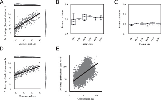
Extended Data Fig. 6 Human stochastic data-based clock predictions correlate significantly with the chronological age. a) The predictions of an Elastic net regression model based on simulated data, correlates significantly (Pearson correlation 0.87, p-value < 1e-16, two-sided test) with the chronological age of the independent healthy biological validation samples (GSE41037, n = 392)78. The simulated data is based on biologically estimated maintenance rates starting with Horvath’s epigenetic clock CpG sites from biological data from a young human blood sample. The x-axis shows the chronological age of the subjects from which blood DNA methylation data was processed. The y-axis shows the predicted simulated age, that is the prediction how often stochastic variation was added to the ground state and is therefore on a different scale and unit than the x-axis. b) The feature size is largely irrelevant for stochastic data-based models in Extended Data Fig. 6a. Predictions of Elastic net regression models trained on more than 500 random CpG sites (features) are significantly correlated with the chronological age. The x-axis shows the number of randomly selected features, that is CpG sites, for the ground state, which were subsequently used to generate data based on stochastic variations (see methods for details). These simulated samples were used to train the Elastic net regression. The y-axis shows the Pearson correlation between the chronological age of the n = 392 healthy samples in GSE41037 ref. 78 (excluding the sample from which the ground state was sampled, and the oldest sample from which maintenance efficiencies were estimated) and the prediction of the independent stochastic-data based model. N = 5 independent experiments are shown. Boxplots are shown with the center line depicting the median, the box limits the bottom, respective top quartiles, and the whiskers the 1.5x interquartile range. c) Verification of Extended Data Fig. 6b). Using the same approach as in Extended Data Fig. 6a, but with randomly shuffled chronological ages shows no significant correlation, indicating that chronological age, and not a confounding variable is correlated with the predictions of the model based on simulated data. The x-axis shows the number of randomly selected features, that is CpG sites, for the ground state, which were subsequently used to generate data based on stochastic variations (see methods for details). These simulated samples were used to train the Elastic net regression. The y-axis shows the Pearson correlation between the permuted chronological age of healthy samples in GSE41037 ref. 78 (excluding the sample from which the ground state was sampled, and the oldest sample from which maintenance efficiencies were estimated) and the prediction of the stochastic-data based model. N = 3 independent experiments are shown. Boxplots are shown with the center line depicting the median, the box limits the bottom, respective top quartiles, and the whiskers the 1.5x interquartile range. d) The same analysis as in Fig. 5a, but the simulated stochastic data were additionally cell-type corrected and then used to train the clock (Pearson correlation 0.81, p < 1e-16, two-sided test). e) The validation of the stochastic data-based clock in Fig. 5 A on 11,146 independent samples from 15 independent datasets (GSE84727, GSE87571, GSE80417, GSE40279, GSE87648, GSE42861, GSE50660, GSE106648, GSE179325, GSE210254, GSE210255, GSE72680, GSE147740, GSE55763, GSE117860) shows a highly significant correlation (Pearson correlation 0.57, p-value < 1e-16).
Extended Data Fig. 6 Human stochastic data-based clock predictions correlate significantly with the chronological age. a) The predictions of an Elastic net regression model based on simulated data, correlates significantly (Pearson correlation 0.87, p-value < 1e-16, two-sided test) with the chronological age of the independent healthy biological validation samples (GSE41037, n = 392)78. The simulated data is based on biologically estimated maintenance rates starting with Horvath’s epigenetic clock CpG sites from biological data from a young human blood sample. The x-axis shows the chronological age of the subjects from which blood DNA methylation data was processed. The y-axis shows the predicted simulated age, that is the prediction how often stochastic variation was added to the ground state and is therefore on a different scale and unit than the x-axis. b) The feature size is largely irrelevant for stochastic data-based models in Extended Data Fig. 6a. Predictions of Elastic net regression models trained on more than 500 random CpG sites (features) are significantly correlated with the chronological age. The x-axis shows the number of randomly selected features, that is CpG sites, for the ground state, which were subsequently used to generate data based on stochastic variations (see methods for details). These simulated samples were used to train the Elastic net regression. The y-axis shows the Pearson correlation between the chronological age of the n = 392 healthy samples in GSE41037 ref. 78 (excluding the sample from which the ground state was sampled, and the oldest sample from which maintenance efficiencies were estimated) and the prediction of the independent stochastic-data based model. N = 5 independent experiments are shown. Boxplots are shown with the center line depicting the median, the box limits the bottom, respective top quartiles, and the whiskers the 1.5x interquartile range. c) Verification of Extended Data Fig. 6b). Using the same approach as in Extended Data Fig. 6a, but with randomly shuffled chronological ages shows no significant correlation, indicating that chronological age, and not a confounding variable is correlated with the predictions of the model based on simulated data. The x-axis shows the number of randomly selected features, that is CpG sites, for the ground state, which were subsequently used to generate data based on stochastic variations (see methods for details). These simulated samples were used to train the Elastic net regression. The y-axis shows the Pearson correlation between the permuted chronological age of healthy samples in GSE41037 ref. 78 (excluding the sample from which the ground state was sampled, and the oldest sample from which maintenance efficiencies were estimated) and the prediction of the stochastic-data based model. N = 3 independent experiments are shown. Boxplots are shown with the center line depicting the median, the box limits the bottom, respective top quartiles, and the whiskers the 1.5x interquartile range. d) The same analysis as in Fig. 5a, but the simulated stochastic data were additionally cell-type corrected and then used to train the clock (Pearson correlation 0.81, p < 1e-16, two-sided test). e) The validation of the stochastic data-based clock in Fig. 5 A on 11,146 independent samples from 15 independent datasets (GSE84727, GSE87571, GSE80417, GSE40279, GSE87648, GSE42861, GSE50660, GSE106648, GSE179325, GSE210254, GSE210255, GSE72680, GSE147740, GSE55763, GSE117860) shows a highly significant correlation (Pearson correlation 0.57, p-value < 1e-16).CC BY · PubMed Central
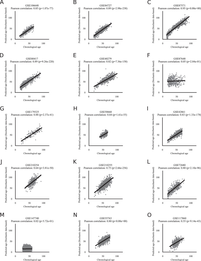
Extended Data Fig. 7 Human stochastic data-based clock predictions correlate significantly with the chronological age of independent validation data. The validation of the stochastic data-based clock starting from a fetal sample (GSM4682890) on 11,146 independent samples from 15 independent datasets a) GSE106648, b) GSE84727, c) GSE87571, d) GSE80417, e) GSE40279, f) GSE87648, g) GSE179325, h) GSE50660, i) GSE42861, j) GSE210254, k) GSE210255, l) GSE72680, m) GSE147740, n) GSE55763, o) GSE117860. See Fig. 5b for a combined plot. The Pearson correlation and its p-value, calculated with a two-sided test, are shown in the figure panels.
Extended Data Fig. 7 Human stochastic data-based clock predictions correlate significantly with the chronological age of independent validation data. The validation of the stochastic data-based clock starting from a fetal sample (GSM4682890) on 11,146 independent samples from 15 independent datasets a) GSE106648, b) GSE84727, c) GSE87571, d) GSE80417, e) GSE40279, f) GSE87648, g) GSE179325, h) GSE50660, i) GSE42861, j) GSE210254, k) GSE210255, l) GSE72680, m) GSE147740, n) GSE55763, o) GSE117860. See Fig. 5b for a combined plot. The Pearson correlation and its p-value, calculated with a two-sided test, are shown in the figure panels.CC BY · PubMed Central
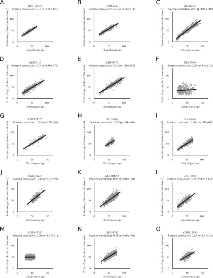
Extended Data Fig. 8 Horvath’s epigenetic age prediction results for the same 15 datasets. Horvath’s epigenetic age prediction on the same 11,146 samples from 15 independent datasets used in Extended Data Fig. 7. a) GSE106648, b) GSE84727, c) GSE87571, d) GSE80417, e) GSE40279, f) GSE87648, g) GSE179325, h) GSE50660, i) GSE42861, j) GSE210254, k) GSE210255, l) GSE72680, m) GSE147740, n) GSE55763, o) GSE117860. Note that GSE40279 and GSE42861 were used during test and training in Horvath’s original publication. Similar to Extended Data Fig. 7GSE87648 and GSE147740 do not show any correlation between the predicted and the chronological age. The Pearson correlation and its p-value, calculated with a two-sided test, are shown in the figure panels.
Extended Data Fig. 8 Horvath’s epigenetic age prediction results for the same 15 datasets. Horvath’s epigenetic age prediction on the same 11,146 samples from 15 independent datasets used in Extended Data Fig. 7. a) GSE106648, b) GSE84727, c) GSE87571, d) GSE80417, e) GSE40279, f) GSE87648, g) GSE179325, h) GSE50660, i) GSE42861, j) GSE210254, k) GSE210255, l) GSE72680, m) GSE147740, n) GSE55763, o) GSE117860. Note that GSE40279 and GSE42861 were used during test and training in Horvath’s original publication. Similar to Extended Data Fig. 7GSE87648 and GSE147740 do not show any correlation between the predicted and the chronological age. The Pearson correlation and its p-value, calculated with a two-sided test, are shown in the figure panels.CC BY · PubMed Central
Extended Data Fig. 9 Stochastic data-based clock predictions correlate significantly with the chronological and biological age of pan-mammalian data. a) The same circle plot as in Fig. 5c, but for Clock 2–4. The Pearson correlation of the relative age of all blood samples of a given species and their predicted age of the stochastic data-based clocks are shown as lines around the circle. Species are shown for which at least 5 blood samples were available. The species are clock-wise sorted by maximum lifespan, starting with Rattus norvegicus (3.8 years) in the center right, and ending with Homo sapiens (122.5 years). The colors within the circle show the taxonomic order of the corresponding species, as listed on the right side. Clock 2 (99% maintenance rate for all CpG sites used in Lu’s pan-mammalian relative age clock15), Clock 3 (CpG site-specific empirically estimated maintenance rates from the oldest sample of Tursiops truncatus for all 37554 CpG sites), and Clock 4 (99% maintenance rate for all 37554 CpG sites) correlate on average highly significantly. b) Example comparison for Fig. 5d. Predictions of Clock 1 for GHRKO (n = 11 biologically independent samples) vs. WT (n = 12 biologically independent samples) liver samples show significantly lower values for GHRKO samples (two-sided adjusted p-value 2.15e-04, full statistics in Source Data 1). Boxplots are shown with the center line depicting the median, the box limits the bottom, respective top quartiles, and the whiskers the 1.5x interquartile range. c) Example comparison for Fig. 5d. Predictions of Clock 1 for Tet3 (n = 8 biologically independent samples) vs. WT (n = 44 biologically independent samples) cerebral cortex samples show significantly lower values for Tet3 samples (two-sided adjusted p-value 2.16e-12, full statistics in Source Data 1). Boxplots are shown with the center line depicting the median, the box limits the bottom, respective top quartiles, and the whiskers the 1.5x interquartile range. d) Example comparison for Fig. 5d. Predictions of Clock 1 for calorie restricted (CR) (n = 59 biologically independent samples) vs. normal fed (n = 36 biologically independent samples) liver samples show significantly lower values for CR samples (two-sided adjusted p-value 3.06e-11, full statistics in Source Data 1). Boxplots are shown with the center line depicting the median, the box limits the bottom, respective top quartiles, and the whiskers the 1.5x interquartile range. e) Example comparison for Fig. 5d. Current-smoker vs. ex-smoker vs. never-smoker aging trajectories are color-coded. The lines show the linear regression model fit of Seaborn’s lmplot function88, and the shadow around the lines the 95% confidence interval. Current-smoker show a steeper aging trajectory (slope) compared to never- or ex-smoker. f) The same as Fig. 5e, but for Clock 2. A multivariate regression of chronological age, the parabiosis treatment, and the interaction shows a significant age variable (p = 6.11e-12), and interaction variable (p = 1.13e-02). The regression model fit with a 95% confidence interval (shadowed area) is shown. g) The same as Fig. 5e, but for Clock 3. A multivariate regression of chronological age, the parabiosis treatment, and the interaction shows a significant age variable (p = 5.6e-09). The regression model fit with a 95% confidence interval (shadowed area) is shown. h) The same as Fig. 5e, but for Clock4. A multivariate regression of chronological age, the parabiosis treatment, and the interaction shows a significant age variable (p = 1.29e-06). The regression model fit with a 95% confidence interval (shadowed area) is shown. Full statistics can be found in Source Data 1.
Extended Data Fig. 9 Stochastic data-based clock predictions correlate significantly with the chronological and biological age of pan-mammalian data. a) The same circle plot as in Fig. 5c, but for Clock 2–4. The Pearson correlation of the relative age of all blood samples of a given species and their predicted age of the stochastic data-based clocks are shown as lines around the circle. Species are shown for which at least 5 blood samples were available. The species are clock-wise sorted by maximum lifespan, starting with Rattus norvegicus (3.8 years) in the center right, and ending with Homo sapiens (122.5 years). The colors within the circle show the taxonomic order of the corresponding species, as listed on the right side. Clock 2 (99% maintenance rate for all CpG sites used in Lu’s pan-mammalian relative age clock15), Clock 3 (CpG site-specific empirically estimated maintenance rates from the oldest sample of Tursiops truncatus for all 37554 CpG sites), and Clock 4 (99% maintenance rate for all 37554 CpG sites) correlate on average highly significantly. b) Example comparison for Fig. 5d. Predictions of Clock 1 for GHRKO (n = 11 biologically independent samples) vs. WT (n = 12 biologically independent samples) liver samples show significantly lower values for GHRKO samples (two-sided adjusted p-value 2.15e-04, full statistics in Source Data 1). Boxplots are shown with the center line depicting the median, the box limits the bottom, respective top quartiles, and the whiskers the 1.5x interquartile range. c) Example comparison for Fig. 5d. Predictions of Clock 1 for Tet3 (n = 8 biologically independent samples) vs. WT (n = 44 biologically independent samples) cerebral cortex samples show significantly lower values for Tet3 samples (two-sided adjusted p-value 2.16e-12, full statistics in Source Data 1). Boxplots are shown with the center line depicting the median, the box limits the bottom, respective top quartiles, and the whiskers the 1.5x interquartile range. d) Example comparison for Fig. 5d. Predictions of Clock 1 for calorie restricted (CR) (n = 59 biologically independent samples) vs. normal fed (n = 36 biologically independent samples) liver samples show significantly lower values for CR samples (two-sided adjusted p-value 3.06e-11, full statistics in Source Data 1). Boxplots are shown with the center line depicting the median, the box limits the bottom, respective top quartiles, and the whiskers the 1.5x interquartile range. e) Example comparison for Fig. 5d. Current-smoker vs. ex-smoker vs. never-smoker aging trajectories are color-coded. The lines show the linear regression model fit of Seaborn’s lmplot function88, and the shadow around the lines the 95% confidence interval. Current-smoker show a steeper aging trajectory (slope) compared to never- or ex-smoker. f) The same as Fig. 5e, but for Clock 2. A multivariate regression of chronological age, the parabiosis treatment, and the interaction shows a significant age variable (p = 6.11e-12), and interaction variable (p = 1.13e-02). The regression model fit with a 95% confidence interval (shadowed area) is shown. g) The same as Fig. 5e, but for Clock 3. A multivariate regression of chronological age, the parabiosis treatment, and the interaction shows a significant age variable (p = 5.6e-09). The regression model fit with a 95% confidence interval (shadowed area) is shown. h) The same as Fig. 5e, but for Clock4. A multivariate regression of chronological age, the parabiosis treatment, and the interaction shows a significant age variable (p = 1.29e-06). The regression model fit with a 95% confidence interval (shadowed area) is shown. Full statistics can be found in Source Data 1.CC BY · PubMed Central
Extended Data Fig. 10 Stochastic data-based clock predictions for pan-mammalian data are robust to the choice of the ground state species. a) Heatmap showing Pearson correlations between the predicted age of Clock 1 trained on the youngest blood sample from species of the corresponding taxonomic order in the columns (Artiodactyla: Tursiops truncatus, Carnivora: Odobenus rosmarus divergens, Lagomorpha: Oryctolagus cuniculus, Monotremata: Tachyglossus aculeatus, Perissodactyla: Equus caballus, Pilosa: Choloepus hoffmanni, Proboscidea: Loxodonta africana, Rodentia: Marmota flaviventris, Sirenia: Trichechus manatus, Suidae: Sus scrofa, Tubulidentata: Orycteropus afer) and the relative age for all species in the rows. The Artiodactyla column corresponds to Fig. 5c. Values are shown for tissues and species for which at least 5 samples were available. b) The box-plots show the distribution of Pearson correlation values of Extended Data Fig. 10a. Clock 1 trained on samples starting from a Monotremata ground state with accumulating variation show on average a lower accuracy. For each of the 12 clocks (based on a different ground state as shown on the x-axis) the n = 57 biologically independent species orders (as indicated in Extended Data Fig. 10a) are shown as dots. Boxplots are shown with the center line depicting the median, the box limits the bottom, respective top quartiles, and the whiskers the 1.5x interquartile range. c) The same as Extended Data Fig. 10b but for Clock 2 trained with 99.99% maintenance rate for all sites of Lu’s pan-mammalian relative age-clock. For each of the 12 clocks (based on a different ground state as shown on the x-axis) the n = 57 biologically independent species orders (as indicated in Extended Data Fig. 10a) are shown as dots. Boxplots are shown with the center line depicting the median, the box limits the bottom, respective top quartiles, and the whiskers the 1.5x interquartile range. d) The same as Extended Data Fig. 10b but for Clock 3 trained on empirically estimated maintenance rates from the species specified in Extended Data Fig. 10a for all 37443 CpG sites. For each of the 12 clocks (based on a different ground state as shown on the x-axis) the n = 57 biologically independent species orders (as indicated in Extended Data Fig. 10a) are shown as dots. Boxplots are shown with the center line depicting the median, the box limits the bottom, respective top quartiles, and the whiskers the 1.5x interquartile range. e) The same as Extended Data Fig. 10b but for Clock 4 train with 99.99% maintenance rate for all 37443 CpG sites. For each of the 12 clocks (based on a different ground state as shown on the x-axis) the n = 57 biologically independent species orders (as indicated in Extended Data Fig. 10a) are shown as dots. Boxplots are shown with the center line depicting the median, the box limits the bottom, respective top quartiles, and the whiskers the 1.5x interquartile range.
Extended Data Fig. 10 Stochastic data-based clock predictions for pan-mammalian data are robust to the choice of the ground state species. a) Heatmap showing Pearson correlations between the predicted age of Clock 1 trained on the youngest blood sample from species of the corresponding taxonomic order in the columns (Artiodactyla: Tursiops truncatus, Carnivora: Odobenus rosmarus divergens, Lagomorpha: Oryctolagus cuniculus, Monotremata: Tachyglossus aculeatus, Perissodactyla: Equus caballus, Pilosa: Choloepus hoffmanni, Proboscidea: Loxodonta africana, Rodentia: Marmota flaviventris, Sirenia: Trichechus manatus, Suidae: Sus scrofa, Tubulidentata: Orycteropus afer) and the relative age for all species in the rows. The Artiodactyla column corresponds to Fig. 5c. Values are shown for tissues and species for which at least 5 samples were available. b) The box-plots show the distribution of Pearson correlation values of Extended Data Fig. 10a. Clock 1 trained on samples starting from a Monotremata ground state with accumulating variation show on average a lower accuracy. For each of the 12 clocks (based on a different ground state as shown on the x-axis) the n = 57 biologically independent species orders (as indicated in Extended Data Fig. 10a) are shown as dots. Boxplots are shown with the center line depicting the median, the box limits the bottom, respective top quartiles, and the whiskers the 1.5x interquartile range. c) The same as Extended Data Fig. 10b but for Clock 2 trained with 99.99% maintenance rate for all sites of Lu’s pan-mammalian relative age-clock. For each of the 12 clocks (based on a different ground state as shown on the x-axis) the n = 57 biologically independent species orders (as indicated in Extended Data Fig. 10a) are shown as dots. Boxplots are shown with the center line depicting the median, the box limits the bottom, respective top quartiles, and the whiskers the 1.5x interquartile range. d) The same as Extended Data Fig. 10b but for Clock 3 trained on empirically estimated maintenance rates from the species specified in Extended Data Fig. 10a for all 37443 CpG sites. For each of the 12 clocks (based on a different ground state as shown on the x-axis) the n = 57 biologically independent species orders (as indicated in Extended Data Fig. 10a) are shown as dots. Boxplots are shown with the center line depicting the median, the box limits the bottom, respective top quartiles, and the whiskers the 1.5x interquartile range. e) The same as Extended Data Fig. 10b but for Clock 4 train with 99.99% maintenance rate for all 37443 CpG sites. For each of the 12 clocks (based on a different ground state as shown on the x-axis) the n = 57 biologically independent species orders (as indicated in Extended Data Fig. 10a) are shown as dots. Boxplots are shown with the center line depicting the median, the box limits the bottom, respective top quartiles, and the whiskers the 1.5x interquartile range.CC BY · PubMed Central

Verification

Claims the paper makes

The claims and statistics of this paper haven’t been checked yet.

Run the check — free, no account needed. It reads the open-access text and checks the sources it cites.

A few free checks a day · papers already verified open instantly · results are public

Self-check

Percentages, sums and reported differences re-computed from the paper’s own numbers.

The self-check needs the paper’s full text.

Citations

Cites

Show all 110 references

Cited by

Sorted by citations

See all 128

Metadata

Authors
Meyer, D. H., & Schumacher, B.
Affiliations
University of Cologne (DE)
Corresponding author
  • Meyer, David H.
  • Schumacher, Björn
Venue
Nature Aging
Published
2024-05-09
Volume
4
Issue
6
Pages
871-885
ISSN
2662-8465 (ISSN-L)
OpenAlex
W4396761662
Cited by
128
References
110
Citations by year
2026: 43 · 2025: 60 · 2024: 21
FWCI
14.96
Type
journal article
Language
en
Open access
Locations
  • Nature Aging (publishedVersion, cc-by)
  • Research Square (acceptedVersion, cc-by)
  • PubMed Central (publishedVersion, cc-by)
  • PubMed (publishedVersion)
Funders
  • EC | Horizon 2020 Framework Programme (H2020-MSCA-ITN-2018 (Healthage and ADDRESS ITNs))
  • John Templeton Foundation (61734)
Topics
  • Life Sciences › Biochemistry, Genetics and Molecular Biology › Aging › Genetics, Aging, and Longevity in Model Organisms
  • Life Sciences › Biochemistry, Genetics and Molecular Biology › Molecular Biology › Epigenetics and DNA Methylation
  • Life Sciences › Biochemistry, Genetics and Molecular Biology › Cell Biology › Telomeres, Telomerase, and Senescence
Keywords
aging clocks, stochastic variability, biological age, chronological age, DNA methylation, transcriptomics, programmed aging, heterochronic parabiosis, caloric restriction, partial reprogramming, smoking, age-related diseases
MeSH terms
Aging, Animals, Biological Clocks, Computer Simulation, Humans, Male, Models, Biological, Parabiosis, Smoking, Stochastic Processes, DNA Methylation, Caloric Restriction, Transcriptome

About these checks

Registry, retraction, Cites and statistics results are computed, not judged, with one exception: a printed reference that no index lists is read once by a model before it counts as a citation error. Claims are extracted by a model and kept only when their quote appears verbatim in the text; each cited source is then checked, with a model’s help, for whether it says what the claim relies on. Those verdicts can be wrong — read the claim’s quote and the cited source before relying on one.

Statistics and arithmetic are recomputed, not judged.

Confidence bands are shown only for fields calibrated on our annotated test set. None is calibrated yet, so no band is shown.

What counts as a claim ›How we measure confidence ›How we check this ›

Are you an author, or do you see a problem with this page? Request a review