CoChat

Feedforward and feedback frequency-dependent interactions in a large-scale laminar network of the primate cortex

Open access
Mejias, Jorge F., Murray, John D., Kennedy, Henry, Wang, Xiao-Jing · 2016 · Science Advances

Published version of a preprint

The DOI matches its Crossref record; 72 of the 72 references it cites were found in a registry or an index.

Abstract

A large-scale laminar network model sheds light on frequency-dependent interactions in the primate cortex.

Overview

The claims and statistics of this paper haven’t been checked yet.

Free: it reads the open-access text and checks the first 5 claims that cite a source we can check. Create a free account to check every claim.

A few free checks a day · papers already verified open instantly · results are public

Integrity signals

Registry

Crossref · 10.1126/sciadv.1601335

Cites

72 of 72 references verified0 citation errors · 0 not checkable

Statistics

Figures

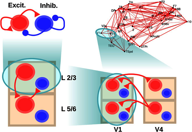
Fig. 1 Scheme of the large-scale model. The scheme shows the four levels considered: a within-layer local microcircuit consisting of an excitatory (Excit.; in red) and an inhibitory (Inhib.; in blue) population (upper left), a laminar circuit with two laminar modules (corresponding to supra- and infragranular layers, lower left), an interareal circuit with laminar-specific projections (lower right), and a large-scale network of 30 cortical areas based on macaque anatomical connectivity (upper right). Each level is anatomically constrained, and its dynamics provide insight into different electrophysiological observations in macaques. Only the connections at each level not shown at a lower level are plotted, for clarity.
Fig. 1 Scheme of the large-scale model. The scheme shows the four levels considered: a within-layer local microcircuit consisting of an excitatory (Excit.; in red) and an inhibitory (Inhib.; in blue) population (upper left), a laminar circuit with two laminar modules (corresponding to supra- and infragranular layers, lower left), an interareal circuit with laminar-specific projections (lower right), and a large-scale network of 30 cortical areas based on macaque anatomical connectivity (upper right). Each level is anatomically constrained, and its dynamics provide insight into different electrophysiological observations in macaques. Only the connections at each level not shown at a lower level are plotted, for clarity.CC BY-NC · PubMed Central
Fig. 2 Local circuit model at the intralaminar level. (A) Scheme of the local circuit (top), with the excitatory and inhibitory population in red and blue, respectively, and examples of the oscillatory activity for an excitatory-inhibitory circuit in layer 2/3 (middle, in green) and layer 5/6 (bottom, in orange). (B) Power spectrum of the firing rate of an isolated layer 2/3 as a function of input strength to the excitatory population. The spectrum of the spontaneous state (with zero input) has been subtracted in each case to highlight changes induced by the input (see main text). As the input increases (which resembles the effect of increasing the contrast of a visual stimulus), the power of gamma rhythms becomes stronger, as in observations by Henrie and Shapley (13). (C) Effect of the input to the excitatory population on the power spectrum peak (left) and frequency (right) of the oscillations, for an isolated layer 2/3 (top) and an isolated layer 5/6 (bottom).
Fig. 2 Local circuit model at the intralaminar level. (A) Scheme of the local circuit (top), with the excitatory and inhibitory population in red and blue, respectively, and examples of the oscillatory activity for an excitatory-inhibitory circuit in layer 2/3 (middle, in green) and layer 5/6 (bottom, in orange). (B) Power spectrum of the firing rate of an isolated layer 2/3 as a function of input strength to the excitatory population. The spectrum of the spontaneous state (with zero input) has been subtracted in each case to highlight changes induced by the input (see main text). As the input increases (which resembles the effect of increasing the contrast of a visual stimulus), the power of gamma rhythms becomes stronger, as in observations by Henrie and Shapley (13). (C) Effect of the input to the excitatory population on the power spectrum peak (left) and frequency (right) of the oscillations, for an isolated layer 2/3 (top) and an isolated layer 5/6 (bottom).CC BY-NC · PubMed Central
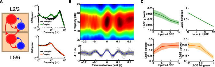
Fig. 3 Cortical area model at the interlaminar level. (A) Scheme of the interlaminar circuit (left panel); self-connections within a given population are omitted in the figure for clarity. Interlaminar connections considered in the model correspond to the strongest projections between layer 2/3 and layer 5/6 as found in experimental studies. Right: Power spectrum of layer 2/3 (top) and layer 5/6 (bottom) in the case of uncoupled, isolated layers (in black, for comparison) and interconnected network (green and orange, respectively). A background input of I = 8 was fed into the excitatory population of both layers. (B) Bottom: A set of 30 traces of activity in layer 5/6 (in gray) and their average (in blue). The central peak of each trace was aligned at zero before averaging. Top: A periodogram of layer 2/3 showing the averaged power for a range of frequencies for the same temporal periods as the layer 5/6 traces. We can see the existence of a strong entrainment of gamma power to alpha phase, as in the experimental findings by Spaak et al. (16). Input was I = 6 for supragranular and I = 8 for infragranular excitatory populations. (C) Effect of injecting external current to the excitatory population of layer 5/6 on the layer 2/3 gamma power and (dimensionless) firing rate (top left and right, respectively) and on layer 5/6 alpha power (bottom left). An inverse relationship between supragranular firing rate and alpha power is observed (bottom right), which highlights a possible link of enhanced alpha rhythms with activity suppression.
Fig. 3 Cortical area model at the interlaminar level. (A) Scheme of the interlaminar circuit (left panel); self-connections within a given population are omitted in the figure for clarity. Interlaminar connections considered in the model correspond to the strongest projections between layer 2/3 and layer 5/6 as found in experimental studies. Right: Power spectrum of layer 2/3 (top) and layer 5/6 (bottom) in the case of uncoupled, isolated layers (in black, for comparison) and interconnected network (green and orange, respectively). A background input of I = 8 was fed into the excitatory population of both layers. (B) Bottom: A set of 30 traces of activity in layer 5/6 (in gray) and their average (in blue). The central peak of each trace was aligned at zero before averaging. Top: A periodogram of layer 2/3 showing the averaged power for a range of frequencies for the same temporal periods as the layer 5/6 traces. We can see the existence of a strong entrainment of gamma power to alpha phase, as in the experimental findings by Spaak et al. (16). Input was I = 6 for supragranular and I = 8 for infragranular excitatory populations. (C) Effect of injecting external current to the excitatory population of layer 5/6 on the layer 2/3 gamma power and (dimensionless) firing rate (top left and right, respectively) and on layer 5/6 alpha power (bottom left). An inverse relationship between supragranular firing rate and alpha power is observed (bottom right), which highlights a possible link of enhanced alpha rhythms with activity suppression.CC BY-NC · PubMed Central
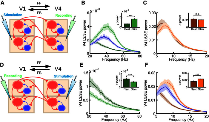
Fig. 4 Microstimulation at the interareal level. (A) Scheme of the interareal projections between two areas (V1 and V4); the anatomical hierarchy ascends from left to right. We inject a current of I = 15 at both supra- and infragranular excitatory populations of V1 and measure at V4. In addition to this input, a background current to excitatory populations in supragranular (I = 2) and infragranular (I = 4) layers in both V1 and V4 is injected to guarantee a minimum level of activity. (B and C) Power spectrum at V4 measured at layer 2/3 (B) and layer 5/6 (C), for resting and stimulation conditions. Insets show the peak value of the power spectrum at supragranular (B) and infragranular (C) layers for the same resting and stimulation conditions. A large increase in gamma power is found, as in the microstimulation experiments by van Kerkoerle et al. (3). (D) Same as (A), but injecting a current of I = 15 at all excitatory populations of V4 and recording in V1. In addition, a background current of I = 1 to all excitatory areas in V1 and V4 is injected to guarantee a minimum of activity. (E and F) Power spectrum at V1 layer 2/3 (E) and layer 5/6 (F) for resting and stimulation conditions. Inset shows the peak value of the power spectrum for these conditions. A large increase in alpha power and a decrease in gamma power were found, in agreement with experimental observations. For (B) and (F), the blue curve corresponds to an isolated area receiving the same input as in the stimulation case, but without its rhythmic component (see main text for details). n.s., not significant. ***P < 0.001.
Fig. 4 Microstimulation at the interareal level. (A) Scheme of the interareal projections between two areas (V1 and V4); the anatomical hierarchy ascends from left to right. We inject a current of I = 15 at both supra- and infragranular excitatory populations of V1 and measure at V4. In addition to this input, a background current to excitatory populations in supragranular (I = 2) and infragranular (I = 4) layers in both V1 and V4 is injected to guarantee a minimum level of activity. (B and C) Power spectrum at V4 measured at layer 2/3 (B) and layer 5/6 (C), for resting and stimulation conditions. Insets show the peak value of the power spectrum at supragranular (B) and infragranular (C) layers for the same resting and stimulation conditions. A large increase in gamma power is found, as in the microstimulation experiments by van Kerkoerle et al. (3). (D) Same as (A), but injecting a current of I = 15 at all excitatory populations of V4 and recording in V1. In addition, a background current of I = 1 to all excitatory areas in V1 and V4 is injected to guarantee a minimum of activity. (E and F) Power spectrum at V1 layer 2/3 (E) and layer 5/6 (F) for resting and stimulation conditions. Inset shows the peak value of the power spectrum for these conditions. A large increase in alpha power and a decrease in gamma power were found, in agreement with experimental observations. For (B) and (F), the blue curve corresponds to an isolated area receiving the same input as in the stimulation case, but without its rhythmic component (see main text for details). n.s., not significant. ***P < 0.001.CC BY-NC · PubMed Central
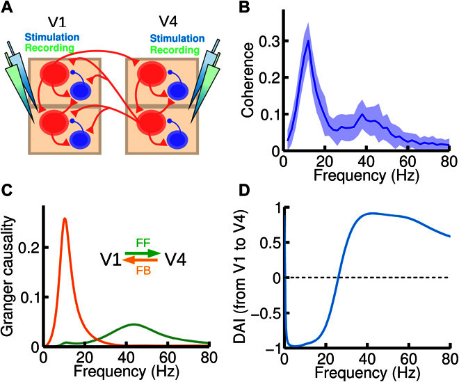
Fig. 5 Frequency-specific FF and FB interactions. (A) We now inject current and record the activity of both areas (V1 and V4). An input current of I = 8 was injected in all excitatory populations of the circuit. (B) Spectral coherence between V1 and V4 activity highlights the existence of two peaks at the alpha and gamma range, respectively. (C) Spectral pairwise GC in the V1-to-V4 (green) and V4-to-V1 (orange) directions, showing that each of the peaks found in (B) corresponds to a particular direction of influence, suggesting that frequency-dependent GC analysis could be used to deduce FF versus FB signaling directionality between areas for which the hierarchical positions are not known anatomically. (D) The DAI profile of the functional connection, which is obtained by normalizing the difference between the two GC profiles in (C), can be used to characterize a directed functional connection between two cortical areas.
Fig. 5 Frequency-specific FF and FB interactions. (A) We now inject current and record the activity of both areas (V1 and V4). An input current of I = 8 was injected in all excitatory populations of the circuit. (B) Spectral coherence between V1 and V4 activity highlights the existence of two peaks at the alpha and gamma range, respectively. (C) Spectral pairwise GC in the V1-to-V4 (green) and V4-to-V1 (orange) directions, showing that each of the peaks found in (B) corresponds to a particular direction of influence, suggesting that frequency-dependent GC analysis could be used to deduce FF versus FB signaling directionality between areas for which the hierarchical positions are not known anatomically. (D) The DAI profile of the functional connection, which is obtained by normalizing the difference between the two GC profiles in (C), can be used to characterize a directed functional connection between two cortical areas.CC BY-NC · PubMed Central
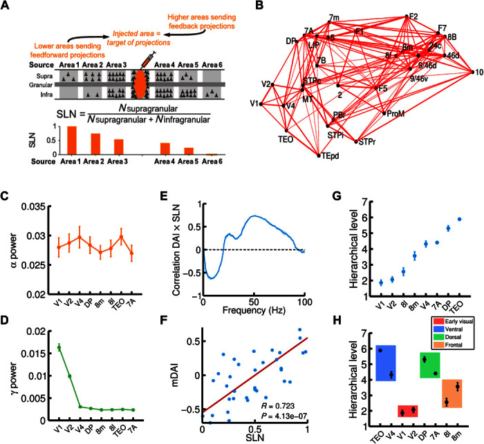
Fig. 6 Large-scale cortical network and functional hierarchy. (A) Illustration of the anatomical tract-tracing technique used to obtain the anatomical large-scale network and, in particular, the fraction of supragranular labeled neurons (or SLNs, see main text for details). A high (low) value of SLN for a given projection indicates that the source area is lower (higher) than the target area (the injected area) in the anatomical hierarchy. (B) 3D plot of the macaque anatomical network obtained (only projections with FLN of >0.005 are plotted, for clarity), with all 30 areas in their spatial positions. Connection strength is indicated by line width. (C and D) alpha (C) and gamma (D) power for eight selected cortical areas of interest (V1, V2, V4, DP, 8m, 8l, TEO, and 7A). (E) Correlation between SLN and DAI, as a function of frequency. The correlation is positive in the gamma range and negative in the alpha range, indicating a prevalent involvement of these rhythms in FF and FB interactions, respectively. (F) Correlation between SLN and the combined DAI across gamma (30 to 70 Hz) and alpha/low-beta (6 to 18 Hz) frequency ranges (named mDAI, see text for details). (G) Functional hierarchy emerging from the frequency-specific interactions in the network and computed using the mDAI values as in Bastos et al. (5). (H) Areas belonging to the same type (early visual, ventral, dorsal, or frontal; indicated by color box) tend to be clustered in the same way as in the experimental observations. For all panels, visual input was simulated with an input current I = 8 to the supragranular excitatory population of V1, and in addition to this input, a background current of I = 6 to all excitatory populations in the network was also considered.
Fig. 6 Large-scale cortical network and functional hierarchy. (A) Illustration of the anatomical tract-tracing technique used to obtain the anatomical large-scale network and, in particular, the fraction of supragranular labeled neurons (or SLNs, see main text for details). A high (low) value of SLN for a given projection indicates that the source area is lower (higher) than the target area (the injected area) in the anatomical hierarchy. (B) 3D plot of the macaque anatomical network obtained (only projections with FLN of >0.005 are plotted, for clarity), with all 30 areas in their spatial positions. Connection strength is indicated by line width. (C and D) alpha (C) and gamma (D) power for eight selected cortical areas of interest (V1, V2, V4, DP, 8m, 8l, TEO, and 7A). (E) Correlation between SLN and DAI, as a function of frequency. The correlation is positive in the gamma range and negative in the alpha range, indicating a prevalent involvement of these rhythms in FF and FB interactions, respectively. (F) Correlation between SLN and the combined DAI across gamma (30 to 70 Hz) and alpha/low-beta (6 to 18 Hz) frequency ranges (named mDAI, see text for details). (G) Functional hierarchy emerging from the frequency-specific interactions in the network and computed using the mDAI values as in Bastos et al. (5). (H) Areas belonging to the same type (early visual, ventral, dorsal, or frontal; indicated by color box) tend to be clustered in the same way as in the experimental observations. For all panels, visual input was simulated with an input current I = 8 to the supragranular excitatory population of V1, and in addition to this input, a background current of I = 6 to all excitatory populations in the network was also considered.CC BY-NC · PubMed Central
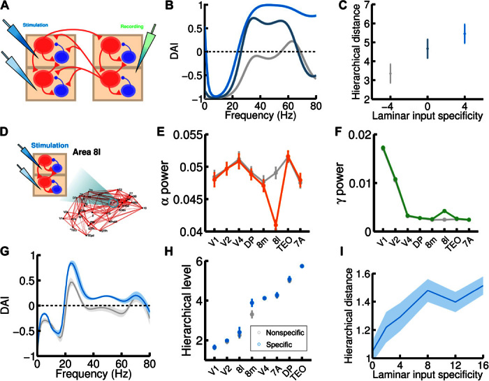
Fig. 7 Mechanistic explanation for the experimentally observed hierarchical jumps. (A) Scheme of the simple two-area circuit considered (we use the same parameters as for the two-area microstimulation protocol); the area on the left, which is lower in the anatomical hierarchy, receives laminar-specific input. (B) The gamma component of the DAI increases as the input to layer 2/3 exceeds input to layer 5/6 for the lower area (ascending curves correspond to input to L2/3E increasing from I = 4 to 6 to 8, and input to L5/6E decreasing from I = 8 to 6 to 4). In the higher area, excitatory populations receive a fixed I = 6 background current. (C) Increases in the hierarchy rank of the higher area as a consequence of the laminar-specific input in (B). The laminar specificity S, defined as the difference between the input to L2/3E and to L5/6E, goes from −4 to 0 to 4 in this example. (D) We follow the same procedure but now injecting laminar-specific current into area 8l within the full 30-area network. (E and F) Changes in alpha (E) and gamma (F) band power as a consequence of the injection of laminar-specific input. Lines in gray correspond to the same input injected at both layers (that is, no laminar-specific input), whereas colored lines correspond to a laminar specificity of S = 8. (G) The spectral DAI profile from 8l to 8m increases in the gamma range as a consequence of the laminar-specific input (gray curve, S = 0; blue curve, S = 8). (H) A hierarchical jump of area 8m is observed, as in the two-area case (gray points, S = 0; blue points, S = 8). (I) We find a robust increase of the hierarchical jump distance with the strength of the laminar specificity of the input. Other parameters and background currents are as in Fig. 6.
Fig. 7 Mechanistic explanation for the experimentally observed hierarchical jumps. (A) Scheme of the simple two-area circuit considered (we use the same parameters as for the two-area microstimulation protocol); the area on the left, which is lower in the anatomical hierarchy, receives laminar-specific input. (B) The gamma component of the DAI increases as the input to layer 2/3 exceeds input to layer 5/6 for the lower area (ascending curves correspond to input to L2/3E increasing from I = 4 to 6 to 8, and input to L5/6E decreasing from I = 8 to 6 to 4). In the higher area, excitatory populations receive a fixed I = 6 background current. (C) Increases in the hierarchy rank of the higher area as a consequence of the laminar-specific input in (B). The laminar specificity S, defined as the difference between the input to L2/3E and to L5/6E, goes from −4 to 0 to 4 in this example. (D) We follow the same procedure but now injecting laminar-specific current into area 8l within the full 30-area network. (E and F) Changes in alpha (E) and gamma (F) band power as a consequence of the injection of laminar-specific input. Lines in gray correspond to the same input injected at both layers (that is, no laminar-specific input), whereas colored lines correspond to a laminar specificity of S = 8. (G) The spectral DAI profile from 8l to 8m increases in the gamma range as a consequence of the laminar-specific input (gray curve, S = 0; blue curve, S = 8). (H) A hierarchical jump of area 8m is observed, as in the two-area case (gray points, S = 0; blue points, S = 8). (I) We find a robust increase of the hierarchical jump distance with the strength of the laminar specificity of the input. Other parameters and background currents are as in Fig. 6.CC BY-NC · PubMed Central

Verification

Claims the paper makes

The claims and statistics of this paper haven’t been checked yet.

Free: it reads the open-access text and checks the first 5 claims that cite a source we can check. Create a free account to check every claim.

A few free checks a day · papers already verified open instantly · results are public

Claims other papers make about this one

Each is checked against this paper’s own text: does it say what the citing paper says it does?

Self-check

Percentages, sums and reported differences re-computed from the paper’s own numbers.

The self-check needs the paper’s full text.

Citations

Cites

Show all 72 references

Cited by

See all 227

Metadata

Authors
Mejias, J. F., Murray, J. D., Kennedy, H., & Wang, X.-J.
Affiliations
  • Center for Neural Science, New York University (NYU), New York, NY 10003, USA.
  • Yale University (US)
  • Lyon 1 Université (FR)
  • New York University Shanghai (CN)
Corresponding author
Wang, Xiao-Jing
Venue
Science Advances
Published
2016-11-04
Volume
2
Issue
11
Pages
e1601335-e1601335
ISSN
2375-2548 (ISSN-L)
OpenAlex
W2491632063
Cited by
227
References
72
Citations by year
2026: 23 · 2025: 31 · 2024: 30 · 2023: 19 · 2022: 23 · 2021: 26 · 2020: 28 · 2019: 21 · 2018: 18 · 2017: 6 · 2016: 2
FWCI
9.97
Type
journal article
Language
en
Open access
Licence
cc-by-nc
Locations
  • Science Advances (publishedVersion, cc-by-nc)
  • bioRxiv (Cold Spring Harbor Laboratory) (acceptedVersion, cc-by-nc)
  • Europe PMC (PubMed Central) (publishedVersion, cc-by-nc)
  • PubMed Central (publishedVersion, cc-by-nc)
  • PubMed (publishedVersion)
Funders
  • Office of Naval Research (ID0ED3AG12440, N00014-13-1-0297)
  • National Institutes of Health (ID0EYCBG12441, R01MH062349)
  • STCSM (ID0ENJBG12442, 14JC1404900, ID0EAQBG12443, 15JC1400104)
  • ANR (ID0ETWBG12444, ANR-11-BSV4-501, ID0EJ6BG12446, ANR-11-IDEX-0007)
  • LABEX CORTEX (ID0E51BG12445, ANR-11-LABX-0042)
Topics
  • Life Sciences › Neuroscience › Cognitive Neuroscience › Neural dynamics and brain function
  • Life Sciences › Neuroscience › Cognitive Neuroscience › Visual perception and processing mechanisms
  • Life Sciences › Neuroscience › Cognitive Neuroscience › Functional Brain Connectivity Studies
Keywords
frequency-dependent interactions, gamma oscillations, alpha oscillations, Granger causality, visual cortex, top-down and bottom-up processing
MeSH terms
Animals, Cerebral Cortex, Macaca, Models, Neurological, Nerve Net, Gamma Rhythm

About these checks

Registry, retraction, Cites and statistics results are computed, not judged, with one exception: a printed reference that no index lists is read once by a model before it counts as a citation error. Claims are extracted by a model and kept only when their quote appears verbatim in the text; each cited source is then checked, with a model’s help, for whether it says what the claim relies on. Those verdicts can be wrong — read the claim’s quote and the cited source before relying on one.

Statistics and arithmetic are recomputed, not judged.

Confidence bands are shown only for fields calibrated on our annotated test set. None is calibrated yet, so no band is shown.

What counts as a claim ›How we measure confidence ›How we check this ›

Are you an author, or do you see a problem with this page? Request a review

Data sources

Bibliographic data: Semantic Scholar, OpenAlex, Crossref.

Contains information from the Semantic Scholar Academic Graph Datasets, made available under the ODC Attribution License (ODC-BY 1.0).

Semantic Scholar’s data is described in: Kinney, R., et al. (2023). The Semantic Scholar Open Data Platform. arXiv:2301.10140.