

One-dimensional organic artificial multi-synapses enabling electronic textile neural network for wearable neuromorphic applications
Open accessThe DOI matches its Crossref record; 56 of the 56 references it cites were found in a registry or an index.
Abstract
We developed 1D multi-synaptic device toward the development of an e-textile neutral network for wearable intelligent applications.
Overview
The claims and statistics of this paper haven’t been checked yet.
Free: it reads the open-access text and checks the first 5 claims that cite a source we can check. Create a free account to check every claim.
Integrity signals
Registry
Cites
Statistics
Figures
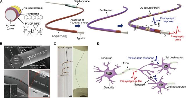

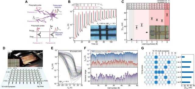

Verification
Claims the paper makes
The claims and statistics of this paper haven’t been checked yet.
Free: it reads the open-access text and checks the first 5 claims that cite a source we can check. Create a free account to check every claim.
Claims other papers make about this one
Each is checked against this paper’s own text: does it say what the citing paper says it does?
The source backs part of the claim, not all of it — or backs it for a different population, condition or comparison.
In the citing paper
“compared with other flexible or stretchable memristive arrays, the f-MDPE offers advantages in terms of energy efficiency and size (Fig. 6g)15,16,18,57–62.”
From Flexible self-rectifying synapse array for energy-efficient edge multiplication in electrocardiogram diagnosis (2025) · cites this paper as [18]
Experimental — accuracy not yet measured
Self-check
Percentages, sums and reported differences re-computed from the paper’s own numbers.
The self-check needs the paper’s full text.
Citations
Cites
Gradient-based learning applied to document recognition
Lecun, Y., Bottou, L., Bengio, Y., & Haffner, P. (1998) · Proceedings of the IEEE · doi:10.1109/5.726791 · Cited by 58,805
Fully integrated wearable sensor arrays for multiplexed in situ perspiration analysis
Gao, W., Emaminejad, S., Nyein, H. Y. Y., Challa, S., Chen, K., Peck, A., Fahad, H. M., Ota, H., Shiraki, H., Kiriya, D., et al. (2016) · Nature · doi:10.1038/nature16521 · Cited by 5,087
Wearable biosensors for healthcare monitoring
Kim, J., Campbell, A. S., de Ávila, B. E.-F., & Wang, J. (2019) · Nature Biotechnology · doi:10.1038/s41587-019-0045-y · Cited by 3,373 · cited 1×
“In addition to this, we should note here that an additional protecting or shielding layer is required to eliminate expected risks related to their contact with the human body while keeping the electrical function of the devices against various environmental conditions ( 45 ).”
Hannun, A. Y., Rajpurkar, P., Haghpanahi, M., Tison, G. H., Bourn, C., Turakhia, M. P., & Ng, A. Y. (2019) · Nature Medicine · doi:10.1038/s41591-018-0268-3 · Cited by 3,148
1.1 Computing's energy problem (and what we can do about it)
Horowitz, M. (2014) · 2014 IEEE International Solid-State Circuits Conference Digest of Technical Papers (ISSCC) · doi:10.1109/isscc.2014.6757323 · Cited by 2,069
Spike Timing–Dependent Plasticity: A Hebbian Learning Rule
Caporale, N., & Dan, Y. (2008) · Annual Review of Neuroscience · doi:10.1146/annurev.neuro.31.060407.125639 · Cited by 1,997
Short-term plasticity and long-term potentiation mimicked in single inorganic synapses
Ohno, T., Hasegawa, T., Tsuruoka, T., Terabe, K., Gimzewski, J. K., & Aono, M. (2011) · Nature Materials · doi:10.1038/nmat3054 · Cited by 1,793 · cited 2×
“Synaptic characteristics and switching mechanism The 1D organic multi-synapses can implement two essential synaptic functions distinguished by a temporal or persistent change in the synaptic weight: (i) short-term plasticity (STP) and (ii) long-term plasticity (31, 32).”
Abbott, L. F., & Regehr, W. G. (2004) · Nature · doi:10.1038/nature03010 · Cited by 1,684 · cited 5×
“1D) ( 30 , 31 ).”
InfluentialMultifunctional wearable devices for diagnosis and therapy of movement disorders
Son, D., Lee, J., Qiao, S., Ghaffari, R., Kim, J., Lee, J. E., Song, C., Kim, S. J., Lee, D. J., Jun, S. W., et al. (2014) · Nature Nanotechnology · doi:10.1038/nnano.2014.38 · Cited by 1,462 · cited 1×
“Thus, the development of wearable devices with various electronic functionalities and suitability for attachment to the human body is necessary ( 1 – 5 ).”
Conductive Fiber‐Based Ultrasensitive Textile Pressure Sensor for Wearable Electronics
Lee, J., Kwon, H., Seo, J., Shin, S., Koo, J. H., Pang, C., Son, S., Kim, J. H., Jang, Y. H., Kim, D. E., et al. (2015) · Advanced Materials · doi:10.1002/adma.201500009 · Cited by 1,152 · cited 1×
“In this regard, various 1D fiber-based devices have been extensively investigated and demonstrated, including energy harvesters ( 9 , 10 ), sensors ( 11 , 12 ), actuators ( 13 ), light-emitting diodes ( 8 , 14 ), transistors ( 15 ), logic circuits ( 16 ), and memories ( 17 , 18 ).”
Cited by
Items 101–185 of 185
Wang, H., Wu, H., Ye, D., Zhao, C., Wu, Q., Wang, S., Zhang, Z., Zeng, M., Wei, H., & Huang, Y. (2024) · Soft Science · doi:10.20517/ss.2024.53 · Cited by 21
Air-stable synaptic devices based on bismuth triiodide and carbon nanotubes
Hao, D., Zhang, J., Li, L., Yang, B., Guo, P., Zhang, S., & Huang, J. D. (2022) · Nano Research · doi:10.1007/s12274-022-4132-x · Cited by 18
Shu, H., Long, H., Sun, H., Li, B., Zhang, H., & Wang, X. (2022) · ACS Omega · doi:10.1021/acsomega.1c06864 · Cited by 19
Ham, S., Jang, J., Koo, D., Gi, S.-G., Kim, D., Jang, S., Kim, N. D., Bae, S., Lee, B., Lee, C., et al. (2024) · Nano Energy · doi:10.1016/j.nanoen.2024.109435 · Cited by 17
Self-citationMemristor-Based CNNs for Detecting Stress Using Brain Imaging Signals
Bak, S., Park, J., Lee, J., & Jeong, J. (2023) · IEEE Transactions on Emerging Topics in Computational Intelligence · doi:10.1109/tetci.2023.3297841 · Cited by 16
Xiang, X., Ma, X., Zhou, L., Sessler, G. M., von Seggern, H., Dali, O. B., Kupnik, M., He, P., Dai, Y., & Zhang, X. (2023) · Advanced Materials Technologies · doi:10.1002/admt.202202130 · Cited by 16
Lee, M., & Jeong, B. (2024) · Advanced Physics Research · doi:10.1002/apxr.202400087 · Cited by 16
Polymer-based smart fibers and textiles for wearable electronics
Hu, S., Wang, L., Yuan, Z., Chen, K., Peng, W., Yin, H. T., Shi, Z., & Yang, G. (2024) · Science China Technological Sciences · doi:10.1007/s11431-024-2738-5 · Cited by 20
Ding, Y., Xu, X., Wu, Y., Zhang, H., Shao, L., Wang, Z., Zhang, H., Zhao, Y. J., & Liu, Y. (2025) · SmartMat · doi:10.1002/smm2.70003 · Cited by 15
“In DG ‐ OFET, the gate terminal emulates the presynaptic terminal, and the channel layer represents the postsynaptic terminal, capable of modulating its behavior in response to gate stimuli, thus enabling signal transmission and learning processes [31].”
A flexible biohybrid reflex arc mimicking neurotransmitter transmission
Shao, L., Luo, S. J., Wang, Z., Xu, X., Yan, Y., Wu, Y., Meng, G., Wei, D., Zhao, Y. J., & Liu, Y. (2022) · Cell Reports Physical Science · doi:10.1016/j.xcrp.2022.100962 · Cited by 15
Kim, T., Lee, W., Kim, S., Lim, D. C., & Kim, Y. (2024) · Advanced Intelligent Systems · doi:10.1002/aisy.202300651 · Cited by 15
Self-citationFerroelectric Transistors: from Materials Innovation to Intelligent Electronic Systems
Li, E., Wang, W., Liu, Y., Wang, R., Luo, C., Zhou, H., Chen, S., Chen, S., Xie, Z., Zhu, K., et al. (2025) · Advanced Materials · doi:10.1002/adma.202515480 · Cited by 14
Kang, H., Kim, H. W., Hong, E. R., & Woo, J. (2022) · Applied Physics Letters · doi:10.1063/5.0086164 · Cited by 14
Chansaengsri, K., Tunhoo, B., Onlaor, K., & Thiwawong, T. (2022) · IEEE Sensors Journal · doi:10.1109/jsen.2022.3217538 · Cited by 13
“The activity affected to signal inconsequentially because the signal performance was higher than the behavior of the movement signal, and the noise canceling was adequate for the artifactassembled system [39], [40], [41].”
BackgroundMicro-cylindrical temperature sensors array via conformal electrohydrodynamic printing
Lai, W., Zhao, C., Wang, H., Wu, Q., Ye, D., & Huang, Y. (2025) · Science China Technological Sciences · doi:10.1007/s11431-024-2903-7 · Cited by 12
Yu, H., Wang, T., Li, Y., Luo, P., & Ni, Y. (2024) · Advanced Electronic Materials · doi:10.1002/aelm.202300702 · Cited by 13
Zhu, L. Q., Wan, X., Lin, J., Chen, P., Luo, Z., Sun, H., Yan, S., Tan, C. L., Yu, Z., & Xu, Y. (2025) · Organic Electronics · doi:10.1016/j.orgel.2025.107199 · Cited by 11
Ke, Y., Mao, L., Jie, W., Gong, T., Huang, W., & Zhang, X. (2021) · ACS Applied Materials & Interfaces · doi:10.1021/acsami.0c21161 · Cited by 11
Humidity-Controlled Preparation of Flexible Porous Carbon Fibers from Block Copolymers
Serrano, J. M., Spiering, G. A., Xu, Z., Croft, Z. L., Guo, D. L., Cao, K., Moore, R. B., & Liu, G. (2022) · ACS Applied Polymer Materials · doi:10.1021/acsapm.2c00534 · Cited by 11
Organic transistors-driven wearable electronics for smart life
Liu, Z., Zhang, C., Xiang, L., Zhang, F., & Di, C. (2024) · Wearable electronics. · doi:10.1016/j.wees.2024.09.004 · Cited by 12
Jin, J., Won, J., Kim, D., Arumugasamy, S. K., Park, S., & Kim, T.-W. (2026) · Nano-Micro Letters · doi:10.1007/s40820-025-02056-w · Cited by 14
“In e-textiles, crossbar-type architectures using 1D fiber devices enable artificial neural networks (ANNs) that support parallel signal processing and pattern recognition [152, 190].”
Self-citationAkbari, M. K., & Zhuiykov, S. (2021) · ACS Applied Materials & Interfaces · doi:10.1021/acsami.1c17584 · Cited by 10
Cho, S., Kundale, S. S., Shim, J., Park, S., Kwak, H., Hoang, A. V., Kim, E., Kim, S., & Park, J. H. (2025) · ACS Applied Materials & Interfaces · doi:10.1021/acsami.4c12694 · Cited by 9
Recent progress of neuromorphic sensory and optoelectronic systems
Nam, S., Kang, D., Jo, J., Kang, D., Park, S. K., & Kim, Y. (2025) · International Journal of Extreme Manufacturing · doi:10.1088/2631-7990/adbb33 · Cited by 12
“Organic semiconductors such as pentacene and p-type {poly[2,5-bis (2 H,5 H)-dione]} are also commonly adopted as channel materials of synaptic devices that emulate the tactile systems [23,37] .”
Liu, Z., Wu, J., Wang, M., Wang, K., Zeng, Y., Dong, X., Wang, K., & Liu, J. (2025) · Advanced Functional Materials · doi:10.1002/adfm.202510021 · Cited by 9
Organic Electrochemical Random Access Memory: From Bio‐Inspired to Bio‐Integrated
Wang, S., Wang, B., Teng, X., Zhao, W., Cao, J., & Ma, W. (2025) · Advanced Materials · doi:10.1002/adma.202515843 · Cited by 10
Bioinspired Vertical Transistors from Artificial Synapse to Neuromorphic System
Li, Y., Huang, Z., Zhang, Y., & Jiang, J. (2023) · physica status solidi (RRL) - Rapid Research Letters · doi:10.1002/pssr.202300181 · Cited by 9
Wearable Fabric μ Brain Enabling On-Garment Edge-Based Sensor Data Processing
Cleary, F., Srisa‐an, W., Gil, B., Kesavan, J., Engel, T., Henshall, D. C., & Balasubramaniam, S. (2022) · IEEE Sensors Journal · doi:10.1109/jsen.2022.3207912 · Cited by 9
“D multisynaptic device to support NNs in an E-textile environment [25].”
BackgroundCao, Y., Meng, J., Li, Q., Wang, T., Zhu, H., Sun, Q., Zhang, D. W., & Chen, L. (2022) · Advanced Electronic Materials · doi:10.1002/aelm.202200909 · Cited by 9
Li, Z., Liu, P., Yang, G., Jia, C., & Zhang, W. (2023) · Physical Chemistry Chemical Physics · doi:10.1039/d3cp01134h · Cited by 9
Ferroelectric‐Gated Hybrid‐Layered Organic Field‐Effect Transistors for Multimode Signal Processing
Liu, J., Zhang, M., Han, W., Du, F., Wu, L., & Fang, X. (2025) · Advanced Functional Materials · doi:10.1002/adfm.202508765 · Cited by 8
Technological trends in medical robotic sensing with soft electronic skin
Zhou, Y., Tang, Y., & Yu, Y. (2023) · Sensors & Diagnostics · doi:10.1039/d3sd00284e · Cited by 8
Ahmed, T., Krishnamurthi, V., Mitchell, A., & Walia, S. (2023) · Advanced Intelligent Systems · doi:10.1002/aisy.202200316 · Cited by 7
Jang, S., Kim, Y., Jeon, J., Ham, S., Choi, S., Yang, J., Kim, S. K., Jeon, S., Jang, J., & Wang, G. (2023) · Journal of Alloys and Compounds · doi:10.1016/j.jallcom.2023.171247 · Cited by 7
Self-citationLee, J., Yoon, T. W., Chung, S., Cho, K., Zhang, G., & Kang, B. (2024) · Advanced Functional Materials · doi:10.1002/adfm.202406229 · Cited by 6
An Organic Ferroelectric Synaptic Transistor
Feng, Z., Wu, J., 杨, W. 伟. Y., 李, W. 伟. L., Feng, G., Zhu, Q., Meng, X., 郭, X. 小. G., Tian, B., Chu, J., et al. (2025) · Chinese Physics Letters · doi:10.1088/0256-307x/42/5/056302 · Cited by 5
Advancing Flexible Optoelectronic Synapses and Neurons with MXene-Integrated Polymeric Platforms
Xu, H., Zeng, X., & Qadir, A. (2025) · Nanomaterials · doi:10.3390/nano15191481 · Cited by 5
“Such devices have enabled significant improvements in computational domains including convolutional processing [163,164], image recognition [165,166], and biosignal monitoring [167,168].”
Micro-cylindrical electrohydrodynamic printing for multilayer electronics
Wu, Q., Wang, H., Ye, D., Li, A., Zhao, C., Wu, H., Lai, W., & Huang, Y. (2025) · Journal of Manufacturing Processes · doi:10.1016/j.jmapro.2025.10.075 · Cited by 5
Weaving Intelligence: Thermally Drawn Multimaterial Fibers Toward AI‐Enabled Smart Textiles
Trung, V. D., Yi, J., Nguyen-Duc, H., Lo, T. N. H., Zhao, W., Dong, C., Sorin, F., Çağlar, B., Wei, L., & Nguyen-Dang, T. (2026) · Advanced Materials · doi:10.1002/adma.73574 · Cited by 5
Convergence of Soft Electronics and Artificial Intelligence: From Materials to Intelligent Systems
Park, H., Choi, G., Yoon, S., Lee, D., & Ko, S. H. (2026) · Nano-Micro Letters · doi:10.1007/s40820-026-02265-x · Cited by 7
Manufacturing strategies for stretchable synaptic transistors
Long, T., Kim, C., Zhao, Y., & Lee, T. (2025) · Wearable electronics. · doi:10.1016/j.wees.2025.07.001 · Cited by 5
Alkali Ion‐Incorporated HfO 2 Dielectrics for Reconfigurable Neuromorphic Computing
Ki, S. Y., Kwak, I. C., Kim, S., Kim, J., Roe, D. G., Kim, S., Kang, J., & Cho, J. H. (2025) · Advanced Functional Materials · doi:10.1002/adfm.202521002 · Cited by 4
Cui, X., Yang, G., Zhang, W., & Jia, C. (2026) · ACS Applied Nano Materials · doi:10.1021/acsanm.5c04952 · Cited by 4
Bioinspired Leaky Integrate‐and‐Fire Neurons Enabled by Reconfigurable Hydrogel Memristors
Lan, R., Zhang, M., Xu, G., Zhang, X., Nie, M., Dai, J., Wang, L., Liu, W., Chang, W., Zhu, G., et al. (2026) · Advanced Materials · doi:10.1002/adma.202520195 · Cited by 6
A single-chip optoelectronic sensor integrated with the human body for tactile perception and memory
Yang, X., Yang, W., Wang, W., Li, K., Li, Y., Zhang, Q., Wang, H., & Hou, C. (2024) · Device · doi:10.1016/j.device.2024.100600 · Cited by 4
Flexible Organic Ferroelectric Synaptic Transistors for Wearable Neuromorphic Systems
Cho, J.-Y., Beak, C., & Lee, S. (2024) · Journal of Flexible and Printed Electronics · doi:10.56767/jfpe.2024.3.1.65 · Cited by 5
“In contrast, ferroelectric transistors based on organic materials can be fabricated using straightforward low-temperature solution processes (below 230°C), rendering them ideal for flexible electronics [19,22-26].”
BackgroundGeng, R., Xie, J., Han, Q., Sun, G., Ma, J., Zhuang, X., & Guo, Q. (2025) · ACS Applied Electronic Materials · doi:10.1021/acsaelm.5c01038 · Cited by 4
He, X., Wang, J., Fu, J., Ming, J., Wang, L., Li, W., Zheng, C., & Ling, H. (2025) · Applied Physics Letters · doi:10.1063/5.0237173 · Cited by 3
Chen, F., Feng, Z., Zhang, S., Min, J., Hu, L., Huang, T., Mei, T., Kim, J., Dong, B., Ma, X., et al. (2025) · Advanced Intelligent Discovery · doi:10.1002/aidi.202500028 · Cited by 3
A Vertical Molecular Synaptic Transistor with Redox-Induced Analog States
Nam, J., Song, M., Lee, H.-S., Lee, C., Kim, D. Y., Wang, G., Kang, K., & Lee, T. (2025) · ACS Nano · doi:10.1021/acsnano.5c17016 · Cited by 3
Self-citationTechnology roadmap from fiber materials to fiber electronics
Zhang, S., Chen, L., Chen, P., Cui, W., Ding, B., Ding, L., Gao, C., Huang, Y., Lei, T., Liao, M., et al. (2026) · National Science Review · doi:10.1093/nsr/nwag368 · Cited by 3
Flexible neuromorphic transistors and their biomimetric sensing application
Jiang, Z., Ke, S., Zhu, Y. J., Zhu, Y., Zhu, L. Q., Wan, C., & Wan, Q. C. (2022) · Acta Physica Sinica · doi:10.7498/aps.71.20220308 · Cited by 3
Piezoelectric Response Analysis of Ferroelectret with Annular Configuration
Xiang, X., Hu, Q., Dai, Y., Zhang, X., & He, P. (2023) · International Journal of Applied Mechanics · doi:10.1142/s1758825123500370 · Cited by 3
Solution-processed Synaptic Transistors Utilizing MXenes as Floating Gate
Zhao, T., Zhao, C., Liu, Y., Yang, L., Mitrović, I. Z., Lim, E. G., & Zhao, C. (2021) · IEEE International Conference on IC Design and Technology (ICICDT) · doi:10.1109/icicdt51558.2021.9626497 · Cited by 3
Three‐Dimensional Garment Architectures for Tactile Embodied Intelligence
Huang, J., Gui, X., Dai, Z., Niu, A., Ma, H., Feng, J., Liu, X., Zhang, H., Zeng, Z., Chen, W., et al. (2026) · Advanced Materials · doi:10.1002/adma.73410 · Cited by 2
Wearable uBrain: Fabric Based-Spiking Neural Network
Cleary, F., Srisa‐an, W., Gil, B., Kesavan, J., Engel, T., Henshall, D. C., & Balasubramaniam, S. (2022) · SETU Waterford Libraries - Open Access Repository · doi:10.48550/arxiv.2202.12984 · Cited by 2
“It is estimated that there is 100 billion neurons in a human brain along with a quadrillion synapses (Herculano-Houzel 2009).”
BackgroundZhu, L.-Y., Yao, Z.-H., Wen, H., Shi, L., & Zhang, X.-L. (2025) · Laser & Optoelectronics Progress · doi:10.3788/lop251012 · Cited by 1
Dual‐Mode Optoelectronic Neuromorphic Architecture for Imaging‐Recognition of Chinese Characters
Zhu, Z., Wang, J., Wang, X., Wang, S., Fu, C., & Luo, L. (2025) · Advanced Optical Materials · doi:10.1002/adom.202502311 · Cited by 2
Fiber-Shaped Optoelectronic Synaptic Device for Neuromorphic Computing in Electronic Textiles
Song, J., Meng, J., Lu, C., Wang, T., Zhu, H., Sun, Q., Chen, P., Zhang, D. W., & Chen, L. (2026) · IEEE Electron Device Letters · doi:10.1109/led.2026.3654557 · Cited by 1
“For example, Ham et al. [20] reported a fiber-shaped multi-synaptic device based on ferroelectric organic transistors fabricated on a 100-µ m Ag wire, functioning as multi-synaptic channels in an e-textile neural network for wearable neuromorphic applications.”
Smart fiber photodetectors based on inorganic semiconductors
Peng, H., Xia, F., Xia, Z., Li, H., & Zhai, T. (2026) · Science China Materials · doi:10.1007/s40843-025-3947-3 · Cited by 1
Tactile and Visual Artificial Synaptic Devices: Progress and Challenges
Chen, Z., Chen, C. P., & Huang, Y. (2026) · Electronic Materials · doi:10.3390/electronicmat7020008 · Cited by 1
“This synapse is composed of ferroelectric organic transistors, in which the ferroelectric transistors form multiple synaptic channels through an interlaced structure [11].”
Design and Manufacturing Principles of Smart Fibers
Wang, Y., Radtke, G., Peters, M. M., Lee, Y., Kawai, M., & Parker, K. K. (2026) · Advanced Materials · doi:10.1002/adma.73959 · Cited by 1
“Adapted and modified with permission [ 299 ].”
Reconfigurable Photoelectric Coaxial Fiber-Based Memristors for Neuromorphic Computing
Li, K., Song, J., Chen, L., He, Y. Q., Meng, J., Wang, T., Zhu, H., Sun, Q., Chen, P., Zhang, D. W., et al. (2026) · ACS Nano · doi:10.1021/acsnano.6c00539 · Cited by 1
Guo, Y., Zhao, J., Liu, J., Zhang, X., Zhang, L., Liu, F., Zhou, J., & Jia, P. (2026) · Chemical Engineering Journal · doi:10.1016/j.cej.2026.181156 · Cited by 1
Advances in Bio‐Integrated Edge Computing Systems for Smart and Connected Health
Kim, G., Yoo, S., Kang, T. W., Huang, Y., & Yeo, W. (2026) · Advanced Materials · doi:10.1002/adma.75390 · Cited by 1
Data transmission and power supply for smart contact lens
Kim, M. (2021) · DR-NTU (Nanyang Technological University) · doi:10.32657/10356/152693
Advanced synaptic transistor device towards AI application in hardware perspective
Zhao, C., Zhao, T., Cao, Y., Liu, Y., Yang, L., Mitrović, I. Z., Lim, E. G., & Zhao, C. (2021) · IEEE International Conference on IC Design and Technology (ICICDT) · doi:10.1109/icicdt51558.2021.9626511
Research on Two-dimensional MXenes Based Synaptic Devices for the Future In-memory Computing
Zhao, C., Zhao, T., Shen, Z., Cao, Y., Liu, Y., Yang, L., Mitrović, I. Z., Lim, E. G., & Zhao, C. (2021) · IEEE International Conference on ASIC (ASICON) · doi:10.1109/asicon52560.2021.9620329
Estratégia de alcance para próteses de membro superior baseada em visão neuromórfica
Gouveia, E. B. (2022) · doi:10.14393/ufu.di.2022.106
“Por possuir baixa dimensionalidade de dados, alto desempenho computacional e baixo consumo de energia, os dispositivos neuromórficos são adequados para aplicações vestíveis [24], [25], aplicações portáteis onde a alta eficiência energética é conveniente [26], [27] e em aplicações onde o alto desempenho computacional é…”
BackgroundWorking Dynamics in Low-dimensional Material-based Neuromorphic Devices
Ahmed, T., Krishnamurthi, V., & Walia, S. (2023) · Royal Society of Chemistry eBooks · doi:10.1039/bk9781839169946-00458
Seo, D., Kang, S., Ryou, H., Shin, M., & Hwang, W. S. (2023) · ACS Omega · doi:10.1021/acsomega.3c05352
Recent Progress of Memristor-based Neuromorphic Computing
Zhou, J. (2024) · Transactions on Computer Science and Intelligent Systems Research · doi:10.62051/1kany131
“The information in the table comes from [23, 10, 9, 12, 5, 18, 20, 21, 22, 14, 17, 19], with the citations listed in the same order as the table.”
BackgroundMoS2 photonic synaptic device development for non-invasive detection of Parkinson’s disease
Divyashree, P., Sharmila, B., & Dwivedi, P. (2024) · Semiconductor Science and Technology · doi:10.1088/1361-6641/ad93f7
Optically Modulated Nanofluidic Ionic Transistor for Neuromorphic Functions
Wang, J., Jiang, Y., Xiong, T., Lu, J., He, X., Yu, P., & Mao, L. (2024) · Angewandte Chemie · doi:10.1002/ange.202418949
Near-infrared artificial synapse based on a pristine InGaAs nanowire synaptic transistor
Xu, H., Yang, Y., Li, Y., Deng, J., Jiang, G., Zhao, X., & Shen, L. (2025) · Nanotechnology · doi:10.1088/1361-6528/ae0594
The novel energy-efficient neuromorphic computing devices
Li, Q., Li, P., & Chen, L. (2025) · Elsevier eBooks · doi:10.1016/b978-0-443-29981-0.00015-x
来, 五., 赵, 晨., 王, 洪., 邬, 清., 叶, 冬., & 黄, 永. (2026) · Scientia Sinica Technologica · doi:10.1360/sst-2025-0348
Song, Y.-S., Chen, Q., Jang, S., Kim, S., Kim, D.-H., Sneha, B., Yeom, J., Bae, S., Moon, B. J., Lee, S.-K., et al. (2026) · Chemical Engineering Journal · doi:10.1016/j.cej.2026.177305
Self-citationSong, G., Zhou, H., Li, Z., Pan, X., Lv, Z., Rao, J., Hao, X., Lü, B., Chen, G., Chen, Y., et al. (2026) · Advanced Materials · doi:10.1002/adma.73462
“Consequently, developing memristive systems that operate in aqueous environments and enable ionic signal transduction is crucial for realizing biologically inspired plausible neuromorphic networks and seamless human–machine interfaces [8–11].”
From Environmental Noise to Computational Degrees of Freedom: Adaptive Neuromorphic Devices
Han, Y., Park, G.-J., Lee, M., Hong, S., Choi, K., & Yoo, H. (2026) · ACS Applied Electronic Materials · doi:10.1021/acsaelm.6c01105
Bio‐inspired vision: From principle, material architectures to system‐level integration
Lin, Z., Xu, M., Ma, X., Yang, W., & Shao, Y. (2026) · FlexMat. · doi:10.1002/flm2.70117
Fibrous Neuromorphic Electronics: From Single Device to All-Fiber System
Lyu, Z., Yu, Q., & Xu, W. (2026) · Nano Letters · doi:10.1021/acs.nanolett.6c02650
Sung, J., An, M., Kim, S., Chung, S., Lee, D., Jeon, Y. U., Park, M., Song, S., Kim, H., Ryu, D. Y., et al. (2026) · Small · doi:10.1002/smll.75609
Nonequilibrium Interfacial Complexation Fibers With Programmable Ionic Memory
Li, T., Jia, H.-B., Nikolaev, K., Chen, H.-R., Wen, X.-Y., Siriaraya, P., Kuwahara, N., Karim, N., Novoselov, K., & Andreeva, D. (2026) · Advances in Materials · doi:10.1002/adma.74913
Wang, W., Cao, G., Yang, G., Zhang, W., & Jia, C. (2026) · Applied Physics Letters · doi:10.1063/5.0336453
Metadata
- Authors
- Ham, S., Kang, M., Jang, S., Jang, J., Choi, S., Kim, T.-W., & Wang, G.
- Affiliations
- Korea University (KR)
- Korea Institute of Science and Technology (KR)
- Jeonbuk National University (KR)
- Corresponding author
- Ham, Seonggil
- Kang, Minji
- Jang, Seonghoon
- Kim, Tae-Wook
- Wang, Gunuk
- Venue
- Science Advances
- Published
- 2020-07-10
- Volume
- 6
- Issue
- 28
- ISSN
- 2375-2548 (ISSN-L)
- PMC
- PMC10662591
- OpenAlex
- W3041554531
- Cited by
- 184
- References
- 56
- Citations by year
- 2026: 24 · 2025: 27 · 2024: 34 · 2023: 36 · 2022: 38 · 2021: 24 · 2020: 1
- FWCI
- 8.49
- Type
- journal article
- Language
- en
- Open access
- gold
- doi.org
- Licence
- Locations
- Science Advances (publishedVersion, cc-by-nc)
- PubMed Central (publishedVersion, cc-by-nc)
- PubMed (publishedVersion)
- Funders
- National Research Foundation of Korea (2019R1A2C2003704, 2019R1A6A3A01095700, 2020R1A2C2010163)
- Samsung Electronics
- the KU-KIST research fund
- Korea University Grant
- Topics
- Physical Sciences › Engineering › Electrical and Electronic Engineering › Advanced Memory and Neural Computing
- Physical Sciences › Engineering › Electrical and Electronic Engineering › Ferroelectric and Negative Capacitance Devices
- Physical Sciences › Engineering › Biomedical Engineering › Advanced Sensor and Energy Harvesting Materials
- Keywords
- smart textiles, cross-point array, MNIST classification
About these checks
Registry, retraction, Cites and statistics results are computed, not judged, with one exception: a printed reference that no index lists is read once by a model before it counts as a citation error. Claims are extracted by a model and kept only when their quote appears verbatim in the text; each cited source is then checked, with a model’s help, for whether it says what the claim relies on. Those verdicts can be wrong — read the claim’s quote and the cited source before relying on one.
Statistics and arithmetic are recomputed, not judged.
Confidence bands are shown only for fields calibrated on our annotated test set. None is calibrated yet, so no band is shown.
What counts as a claim ›How we measure confidence ›How we check this ›
Are you an author, or do you see a problem with this page? Request a review
Data sources
Bibliographic data: Semantic Scholar, OpenAlex, Crossref.
Contains information from the Semantic Scholar Academic Graph Datasets, made available under the ODC Attribution License (ODC-BY 1.0).
Semantic Scholar’s data is described in: Kinney, R., et al. (2023). The Semantic Scholar Open Data Platform. arXiv:2301.10140.
