

The DOI matches its Crossref record; 53 of the 53 references it cites were found in a registry or an index.
Broadband Criticality of Human Brain Network Synchronization
Open accessAbstract
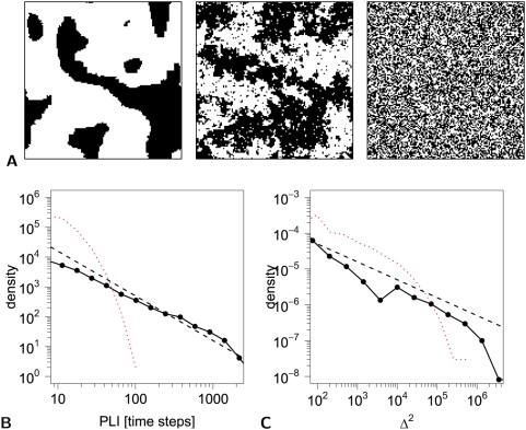
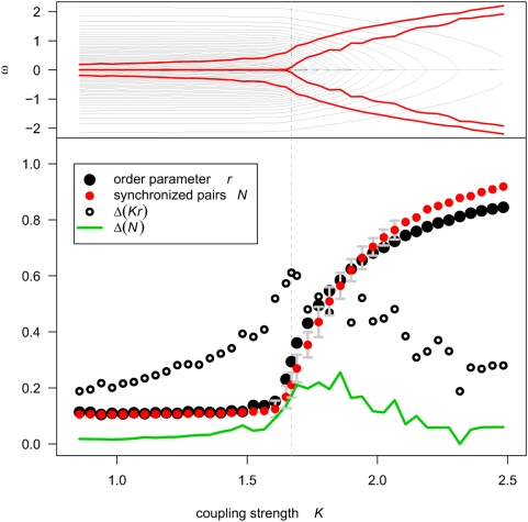
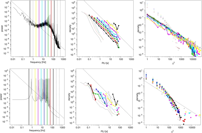
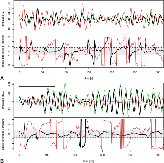
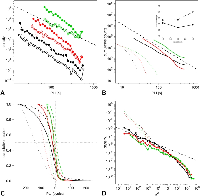
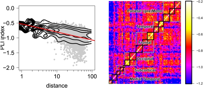
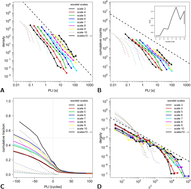
Self-organized criticality is an attractive model for human brain dynamics, but there has been little direct evidence for its existence in large-scale systems measured by neuroimaging. In general, critical systems are associated with fractal or power law scaling, long-range correlations in space and time, and rapid reconfiguration in response to external inputs. Here, we consider two measures of phase synchronization: the phase-lock interval, or duration of coupling between a pair of (neurophysiological) processes, and the lability of global synchronization of a (brain functional) network. Using computational simulations of two mechanistically distinct systems displaying complex dynamics, the Ising model and the Kuramoto model, we show that both synchronization metrics have power law probability distributions specifically when these systems are in a critical state. We then demonstrate power law scaling of both pairwise and global synchronization metrics in functional MRI and magnetoencephalographic data recorded from normal volunteers under resting conditions. These results strongly suggest that human brain functional systems exist in an endogenous state of dynamical criticality, characterized by a greater than random probability of both prolonged periods of phase-locking and occurrence of large rapid changes in the state of global synchronization, analogous to the neuronal "avalanches" previously described in cellular systems. Moreover, evidence for critical dynamics was identified consistently in neurophysiological systems operating at frequency intervals ranging from 0.05-0.11 to 62.5-125 Hz, confirming that criticality is a property of human brain functional network organization at all frequency intervals in the brain's physiological bandwidth.
Overview
The claims and statistics of this paper haven’t been checked yet.
Run the check — free, no account needed. It reads the open-access text and checks the sources it cites.
Integrity signals
Registry
Cites
Statistics
Figures
Verification
Claims the paper makes
The claims and statistics of this paper haven’t been checked yet.
Run the check — free, no account needed. It reads the open-access text and checks the sources it cites.
Claims other papers make about this one
Each is checked against this paper’s own text: does it say what the citing paper says it does?
The source backs part of the claim, not all of it — or backs it for a different population, condition or comparison.
In the citing paper
“Several lines of evidence point to fractal-like (1/f) self-similarity over different spatio-temporal scales in brain dynamics and structure [76,77].”
From Consciousness in the universe (2014) · cites this paper as [77]
Experimental — accuracy not yet measuredThe cited source says what the claim attributes to it.
In the citing paper
“there does appear to be evidence for some kind of scale-invariance in neurophysiological processes (Section 3.2 [76,77]).”
From Consciousness in the universe (2014) · cites this paper as [77]
Self-check
Percentages, sums and reported differences re-computed from the paper’s own numbers.
The self-check needs the paper’s full text.
Citations
Cites
Collective dynamics of ‘small-world’ networks
Watts, D. J., & Strogatz, S. H. (1998) · Nature · doi:10.1038/30918 · Cited by 43,060
Tzourio-Mazoyer, N., Landeau, B., Papathanassiou, D., Crivello, F., Etard, O., Delcroix, N., Mazoyer, B., & Joliot, M. (2002) · NeuroImage · doi:10.1006/nimg.2001.0978 · Cited by 16,319
Multimodel Inference: Understanding AIC and BIC in Model Selection
Burnham, K. P., & Anderson, D. R. (2004) · Sociological Methods & Research · doi:10.1177/0049124104268644 · Cited by 11,648
PIKOVSKY, A. S., Rosenblum, M., & Kurths, J. (2001) · Cambridge University Press eBooks · doi:10.1017/cbo9780511755743 · Cited by 8,250
Chemical Oscillations, Waves, and Turbulence
Kuramoto, Y. (1984) · Springer series in synergetics · doi:10.1007/978-3-642-69689-3 · Cited by 7,242
Crystal Statistics. I. A Two-Dimensional Model with an Order-Disorder Transition
Onsager, L. (1944) · Physical Review · doi:10.1103/physrev.65.117 · Cited by 6,634
Synchronization a universal concept in nonlinear sciences
PIKOVSKY, A. S., Rosenblum, M. G., & Kurths, J. (2001) · Cited by 5,640
A mechanism for cognitive dynamics: neuronal communication through neuronal coherence.
Fries, P. (2005) · Trends in Cognitive Sciences · doi:10.1016/j.tics.2005.08.011 · Cited by 4,284
Gray, C. M., König, P., Engel, A. K., & Singer, W. (1989) · Nature · doi:10.1038/338334a0 · Cited by 4,183
Beitrag zur Theorie des Ferromagnetismus
Ising, E. (1925) · Zeitschrift für Physik · doi:10.1007/bf02980577 · Cited by 3,871
Cited by
Sorted by citations
Complex brain networks: graph theoretical analysis of structural and functional systems
Bullmore, E., & Sporns, O. (2009) · Nature Reviews Neuroscience · doi:10.1038/nrn2575 · Cited by 11,820
Self-citationThe free-energy principle: a unified brain theory?
Friston, K. (2010) · Nature Reviews Neuroscience · doi:10.1038/nrn2787 · Cited by 8,120
Functional and Effective Connectivity: A Review
Friston, K. J. (2011) · Brain Connectivity · doi:10.1089/brain.2011.0008 · Cited by 3,415
The economy of brain network organization
Bullmore, E., & Sporns, O. (2012) · Nature Reviews Neuroscience · doi:10.1038/nrn3214 · Cited by 3,284
Self-citationThe role of the posterior cingulate cortex in cognition and disease
Leech, R., & Sharp, D. J. (2014) · Brain · doi:10.1093/brain/awt162 · Cited by 2,247
Gut microbiome alterations in Alzheimer’s disease
Vogt, N. M., Kerby, R. L., Dill-McFarland, K. A., Harding, S. J., Merluzzi, A. P., Johnson, S. C., Carlsson, C. M., Asthana, S., Zetterberg, H., Blennow, K., et al. (2017) · Scientific Reports · doi:10.1038/s41598-017-13601-y · Cited by 2,137
The human connectome: a complex network
Sporns, O. (2011) · Annals of the New York Academy of Sciences · doi:10.1111/j.1749-6632.2010.05888.x · Cited by 1,440
Emergent complex neural dynamics
Chialvo, D. R. (2010) · Nature Physics · doi:10.1038/nphys1803 · Cited by 1,165
Brain Graphs: Graphical Models of the Human Brain Connectome
Bullmore, E. T., & Bassett, D. S. (2011) · Annual Review of Clinical Psychology · doi:10.1146/annurev-clinpsy-040510-143934 · Cited by 1,165
Self-citationThe Kuramoto model in complex networks
Rodrigues, F. A., Peron, T., Ji, P., & Kurths, J. (2015) · Physics Reports · doi:10.1016/j.physrep.2015.10.008 · Cited by 1,064
Hameroff, S., & Penrose, R. (2014) · Physics of Life Reviews · doi:10.1016/j.plrev.2013.08.002 · Cited by 983
“Neurons have a rich and uniquely organized cytoskeleton, the major components being microtubules, well-positioned and uniquely arrayed (e.g. in dendrites and soma) to mediate consciousness and regulate firing.”
BackgroundHuman brain networks in health and disease
Bassett, D. S., & Bullmore, E. T. (2009) · Current Opinion in Neurology · doi:10.1097/wco.0b013e32832d93dd · Cited by 922
Self-citationTime-resolved resting-state brain networks
Zalesky, A., Fornito, A., Cocchi, L., Gollo, L. L., & Breakspear, M. (2014) · Proceedings of the National Academy of Sciences · doi:10.1073/pnas.1400181111 · Cited by 753
Graph analysis of the human connectome: Promise, progress, and pitfalls
Fornito, A., Zalesky, A., & Breakspear, M. (2013) · NeuroImage · doi:10.1016/j.neuroimage.2013.04.087 · Cited by 743
Criticality in Large-Scale Brain fMRI Dynamics Unveiled by a Novel Point Process Analysis
Tagliazucchi, E., Balenzuela, P., Fraiman, D., & Chialvo, D. R. (2012) · Frontiers in Physiology · doi:10.3389/fphys.2012.00015 · Cited by 738
Ongoing Cortical Activity at Rest: Criticality, Multistability, and Ghost Attractors
Deco, G., & Jirsa, V. (2012) · Journal of Neuroscience · doi:10.1523/jneurosci.2523-11.2012 · Cited by 704
Hierarchical modularity in human brain functional networks
David Meunier, A. (2009) · Frontiers in Neuroinformatics · doi:10.3389/neuro.11.037.2009 · Cited by 689
Can structure predict function in the human brain?
Honey, C. J., Thivierge, J.-P., & Sporns, O. (2010) · NeuroImage · doi:10.1016/j.neuroimage.2010.01.071 · Cited by 629
The Functional Benefits of Criticality in the Cortex
Shew, W. L., & Plenz, D. (2013) · The Neuroscientist · doi:10.1177/1073858412445487 · Cited by 607
EEG microstate sequences in healthy humans at rest reveal scale-free dynamics.
Van De Ville, D., Britz, J., & Michel, C. M. (2010) · Proceedings of the National Academy of Sciences · doi:10.1073/pnas.1007841107 · Cited by 606
Understanding complexity in the human brain
Bassett, D. S., & Gazzaniga, M. S. (2011) · Trends in Cognitive Sciences · doi:10.1016/j.tics.2011.03.006 · Cited by 572
Computational psychiatry: the brain as a phantastic organ
Friston, K. J., Stephan, K. E., Montague, R., & Dolan, R. J. (2014) · The Lancet Psychiatry · doi:10.1016/s2215-0366(14)70275-5 · Cited by 531
Criticality in the brain: A synthesis of neurobiology, models and cognition
Cocchi, L., Gollo, L. L., Zalesky, A., & Breakspear, M. J. (2017) · Progress in Neurobiology · doi:10.1016/j.pneurobio.2017.07.002 · Cited by 555
Being Critical of Criticality in the Brain
Beggs, J. M., & Timme, N. M. (2012) · Frontiers in Physiology · doi:10.3389/fphys.2012.00163 · Cited by 505
Cognitive relevance of the community structure of the human brain functional coactivation network
Crossley, N. A., Mechelli, A., Vértes, P. E., Winton‐Brown, T., Patel, A. X., Ginestet, C. E., McGuire, P. K., & Bullmore, E. T. (2013) · Proceedings of the National Academy of Sciences · doi:10.1073/pnas.1220826110 · Cited by 457
Self-citationSelf-organized criticality as a fundamental property of neural systems
Hesse, J., & Gross, T. (2014) · Frontiers in Systems Neuroscience · doi:10.3389/fnsys.2014.00166 · Cited by 440
Haimovici, A., Tagliazucchi, E., Balenzuela, P., & Chialvo, D. R. (2013) · Physical Review Letters · doi:10.1103/physrevlett.110.178101 · Cited by 438
Cognitive fitness of cost-efficient brain functional networks
Bassett, D. S., Bullmore, E. T., Meyer‐Lindenberg, A., Apud, J. A., Weinberger, D. R., & Coppola, R. (2009) · Proceedings of the National Academy of Sciences · doi:10.1073/pnas.0903641106 · Cited by 429
Self-citationCognitive effort drives workspace configuration of human brain functional networks
Kitzbichler, M. G., Henson, R. N. A., Smith, M. L., Nathan, P. J., & Bullmore, E. T. (2011) · The Journal of Neuroscience · doi:10.1523/jneurosci.0440-11.2011 · Cited by 427
Self-citationThe graphical brain: Belief propagation and active inference
Friston, K. J., Parr, T., & de Vries, B. (2017) · Network Neuroscience · doi:10.1162/netn_a_00018 · Cited by 415
Bassett, D. S., Greenfield, D. L., Meyer‐Lindenberg, A., Weinberger, D. R., Moore, S. W., & Bullmore, E. T. (2010) · PLoS Computational Biology · doi:10.1371/journal.pcbi.1000748 · Cited by 401
Self-citationLeonardi, N., Richiardi, J., Gschwind, M., Simioni, S., Annoni, J., Schluep, M., Vuilleumier, P. O., & Ville, D. V. D. (2013) · NeuroImage · doi:10.1016/j.neuroimage.2013.07.019 · Cited by 401
Poil, S., Hardstone, R., Mansvelder, H. D., & Linkenkaer‐Hansen, K. (2012) · Journal of Neuroscience · doi:10.1523/jneurosci.5990-11.2012 · Cited by 397
Periodic changes in fMRI connectivity
Handwerker, D. A., Roopchansingh, V., González-Castillo, J., & Bandettini, P. A. (2012) · NeuroImage · doi:10.1016/j.neuroimage.2012.06.078 · Cited by 360
Boccaletti, S., Pisarchik, A. N., del Genio, C. I., & Amann, A. (2018) · Cambridge University Press eBooks · doi:10.1017/9781107297111 · Cited by 359
Mathematical framework for large-scale brain network modeling in The Virtual Brain
Sanz-Leon, P., Knock, S. A., Spiegler, A., & Jirsa, V. K. (2015) · NeuroImage · doi:10.1016/j.neuroimage.2015.01.002 · Cited by 356
Conserved and variable architecture of human white matter connectivity
Bassett, D., Brown, J. A., Deshpande, V., Carlson, J., & Grafton, S. T. (2011) · NeuroImage · doi:10.1016/j.neuroimage.2010.09.006 · Cited by 380
Griffiths phases and the stretching of criticality in brain networks
Moretti, P., & Muñoz, M. A. (2013) · Nature Communications · doi:10.1038/ncomms3521 · Cited by 360
Neuronal Avalanches in the Resting MEG of the Human Brain
Shriki, O., Alstott, J., Carver, F. W., Holroyd, T., Henson, R. N., Smith, M. L., Coppola, R., Bullmore, E. T., & Plenz, D. (2013) · Journal of Neuroscience · doi:10.1523/jneurosci.4286-12.2013 · Cited by 346
Self-citationGlerean, E., Salmi, J., Lahnakoski, J. M., Jääskeläinen, I. P., & Sams, M. (2012) · Brain Connectivity · doi:10.1089/brain.2011.0068 · Cited by 325
Cabral, J., Luckhoo, H., Woolrich, M. W., Joensson, M., Mohseni, H., Baker, A. P., Kringelbach, M. L., & Deco, G. (2013) · NeuroImage · doi:10.1016/j.neuroimage.2013.11.047 · Cited by 320
Construct validation of a DCM for resting state fMRI
Razi, A., Kahan, J., Rees, G. E., & Friston, K. J. (2014) · NeuroImage · doi:10.1016/j.neuroimage.2014.11.027 · Cited by 287
Friston, K. J., Li, B., Daunizeau, J., & Stephan, K. E. (2011) · NeuroImage · doi:10.1016/j.neuroimage.2010.12.039 · Cited by 283
Metastable chimera states in community-structured oscillator networks
Shanahan, M. (2010) · Chaos An Interdisciplinary Journal of Nonlinear Science · doi:10.1063/1.3305451 · Cited by 275
How critical is brain criticality?
O’Byrne, J., & Jerbi, K. (2022) · Trends in Neurosciences · doi:10.1016/j.tins.2022.08.007 · Cited by 283
Rubinov, M., Sporns, O., Thivierge, J., & Breakspear, M. J. (2011) · PLoS Computational Biology · doi:10.1371/journal.pcbi.1002038 · Cited by 265
Cardiac and Respiratory Patterns Synchronize between Persons during Choir Singing
Müller, V., & Lindenberger, U. (2011) · PLoS ONE · doi:10.1371/journal.pone.0024893 · Cited by 256
Consciousness-specific dynamic interactions of brain integration and functional diversity
Luppi, A. I., Craig, M. M., Pappas, I., Finoia, P., Williams, G. B., Allanson, J., Pickard, J. D., Owen, A. M., Naci, L., Menon, D. K., et al. (2019) · Nature Communications · doi:10.1038/s41467-019-12658-9 · Cited by 251
Fractals in the nervous system: conceptual implications for theoretical neuroscience
Werner, G. (2010) · Frontiers in Physiology · doi:10.3389/fphys.2010.00015 · Cited by 252
Resting-State Temporal Synchronization Networks Emerge from Connectivity Topology and Heterogeneity
Ponce‐Alvarez, A., Deco, G., Hagmann, P., Romani, G. L., Mantini, D., & Corbetta, M. (2015) · PLoS Computational Biology · doi:10.1371/journal.pcbi.1004100 · Cited by 244
Atasoy, S., Roseman, L., Kaelen, M., Kringelbach, M. L., Deco, G., & Carhart-Harris, R. L. (2017) · Scientific Reports · doi:10.1038/s41598-017-17546-0 · Cited by 214
Emergent Criticality in Complex Turing B‐Type Atomic Switch Networks
Stieg, A. Z., Avizienis, A. V., Sillin, H. O., Martin‐Olmos, C., Aono, M., & Gimzewski, J. K. (2011) · Advanced Materials · doi:10.1002/adma.201103053 · Cited by 212
Hellyer, P. J., Shanahan, M., Scott, G., Wise, R. J. S., Sharp, D. J., & Leech, R. (2014) · Journal of Neuroscience · doi:10.1523/jneurosci.1853-13.2014 · Cited by 205
Ising-like dynamics in large-scale functional brain networks
Fraiman, D., Balenzuela, P., Foss, J., & Chialvo, D. R. (2009) · Physical Review E · doi:10.1103/physreve.79.061922 · Cited by 205
Spike Avalanches Exhibit Universal Dynamics across the Sleep-Wake Cycle
Ribeiro, T. L., Copelli, M., Caixeta, F. V., Belchior, H., Chialvo, D. R., Nicolelis, M. A. L., & Ribeiro, S. T. G. (2010) · PLoS ONE · doi:10.1371/journal.pone.0014129 · Cited by 200
Failure of Adaptive Self-Organized Criticality during Epileptic Seizure Attacks
Meisel, C., Storch, A., Hallmeyer‐Elgner, S., Bullmore, E. T., & Groß, T. (2012) · PLoS Computational Biology · doi:10.1371/journal.pcbi.1002312 · Cited by 192
Self-citationBistability and Non-Gaussian Fluctuations in Spontaneous Cortical Activity
Freyer, F., Aquino, K., Robinson, P. A., Ritter, P., & Breakspear, M. (2009) · Journal of Neuroscience · doi:10.1523/jneurosci.0754-09.2009 · Cited by 189
Why Brain Criticality Is Clinically Relevant: A Scoping Review
Zimmern, V. (2020) · Frontiers in Neural Circuits · doi:10.3389/fncir.2020.00054 · Cited by 208
Hellyer, P. J., Scott, G., Shanahan, M., Sharp, D. J., & Leech, R. (2015) · Journal of Neuroscience · doi:10.1523/jneurosci.4648-14.2015 · Cited by 187
Modeling complex systems with adaptive networks
Sayama, H., Pestov, I., Schmidt, J., Bush, B. J., Wong, C., Yamanoi, J., & Groß, T. (2013) · Computers & Mathematics with Applications · doi:10.1016/j.camwa.2012.12.005 · Cited by 187
Local measures of information storage in complex distributed computation
Lizier, J. T., Prokopenko, M., & Zomaya, A. Y. (2012) · Information Sciences · doi:10.1016/j.ins.2012.04.016 · Cited by 180
A Functional Cartography of Cognitive Systems
Mattar, M. G., Cole, M. W., Thompson‐Schill, S. L., & Bassett, D. S. (2015) · PLoS Computational Biology · doi:10.1371/journal.pcbi.1004533 · Cited by 177
Endogenous Human Brain Dynamics Recover Slowly Following Cognitive Effort
Barnes, A., Bullmore, E. T., & Suckling, J. (2009) · PLoS ONE · doi:10.1371/journal.pone.0006626 · Cited by 174
Self-citationPalva, J. M., & Palva, S. (2012) · NeuroImage · doi:10.1016/j.neuroimage.2012.02.060 · Cited by 163
Intra- and Inter-Brain Synchronization during Musical Improvisation on the Guitar
Müller, V., Sänger, J., & Lindenberger, U. (2013) · PLoS ONE · doi:10.1371/journal.pone.0073852 · Cited by 174
Outline of a general theory of behavior and brain coordination
Kelso, J. A. S., Dumas, G., & Tognoli, E. (2012) · Neural Networks · doi:10.1016/j.neunet.2012.09.003 · Cited by 173
Cytoskeletal signaling: is memory encoded in microtubule lattices by CaMKII phosphorylation?
Craddock, T. J. A., Tuszynski, J. A., & Hameroff, S. (2012) · PLoS Computational Biology · doi:10.1371/journal.pcbi.1002421 · Cited by 160
Voltage imaging of waking mouse cortex reveals emergence of critical neuronal dynamics
Scott, G., Fagerholm, E. D., Mutoh, H., Leech, R., Sharp, D. J., Shew, W. L., & Knöpfel, T. (2014) · The Journal of Neuroscience · doi:10.1523/jneurosci.3474-14.2014 · Cited by 158
Adaptive self-organization in a realistic neural network model
Meisel, C., & Groß, T. (2009) · Physical Review E · doi:10.1103/physreve.80.061917 · Cited by 146
Fading Signatures of Critical Brain Dynamics during Sustained Wakefulness in Humans
Meisel, C., Olbrich, E., Shriki, O., & Achermann, P. (2013) · Journal of Neuroscience · doi:10.1523/jneurosci.1516-13.2013 · Cited by 148
Spontaneous brain activity as a source of ideal 1/f noise
Allegrini, P., Menicucci, D., Bedini, R., Fronzoni, L., Gemignani, A., Paolo Grigolini, A., West, B. J., & Paradisi, P. (2009) · Physical Review E · doi:10.1103/physreve.80.061914 · Cited by 142
Graph properties of synchronized cortical networks during visual working memory maintenance
Palva, S., Monto, S., & Palva, J. M. (2009) · NeuroImage · doi:10.1016/j.neuroimage.2009.11.031 · Cited by 141
Meisel, C., Schulze‐Bonhage, A., Freestone, D. R., Cook, M. J., Achermann, P., & Plenz, D. (2015) · Proceedings of the National Academy of Sciences · doi:10.1073/pnas.1513716112 · Cited by 138
Self-similar correlation function in brain resting-state functional magnetic resonance imaging
Expert, P., Lambiotte, R., Chialvo, D. R., Christensen, K., Jensen, H. J., Sharp, D. J., & Turkheimer, F. (2010) · Journal of The Royal Society Interface · doi:10.1098/rsif.2010.0416 · Cited by 137
Wang, D. J. J., Jann, K., Fan, C., Qiao, Y., Zang, Y., Lu, H., & Yang, Y. (2018) · Frontiers in Neuroscience · doi:10.3389/fnins.2018.00352 · Cited by 140
Learning function from structure in neuromorphic networks
Suárez, L. E., Richards, B. A., Lajoie, G., & Mišić, B. (2021) · Nature Machine Intelligence · doi:10.1038/s42256-021-00376-1 · Cited by 137
Computational and dynamic models in neuroimaging
Friston, K. J., & Dolan, R. J. (2010) · NeuroImage · doi:10.1016/j.neuroimage.2009.12.068 · Cited by 131
Generic aspects of complexity in brain imaging data and other biological systems
Bullmore, E. T., Barnes, A., Bassett, D. S., Fornito, A., Kitzbichler, M. G., David Meunier, A., & Suckling, J. (2009) · NeuroImage · doi:10.1016/j.neuroimage.2009.05.032 · Cited by 136
Self-citationHakim, U., Felice, S. D., Pinti, P., Zhang, X., Noah, J. A., Ono, Y., Burgess, P. W., Hamilton, A. F. D. C., Hirsch, J., & Tachtsidis, I. (2023) · NeuroImage · doi:10.1016/j.neuroimage.2023.120354 · Cited by 131
Betzel, R. F., Medaglia, J. D., Kahn, A. E., Soffer, J., Schonhaut, D. R., & Bassett, D. S. (2019) · Nature Biomedical Engineering · doi:10.1038/s41551-019-0404-5 · Cited by 129
How anatomy shapes dynamics: a semi-analytical study of the brain at rest by a simple spin model
Deco, G., Senden, M., & Jirsa, V. (2012) · Frontiers in Computational Neuroscience · doi:10.3389/fncom.2012.00068 · Cited by 132
Eigenmodes of brain activity: Neural field theory predictions and comparison with experiment
Robinson, P. A., Zhao, X., Aquino, K. M., Griffiths, J. D., Sarkar, S., & Mehta-Pandejee, G. (2016) · NeuroImage · doi:10.1016/j.neuroimage.2016.04.050 · Cited by 129
Kaiser, M. (2010) · Frontiers in Neuroinformatics · doi:10.3389/fninf.2010.00008 · Cited by 126
Topological and Dynamical Complexity of Random Neural Networks
Wainrib, G., & Touboul, J. (2013) · Physical Review Letters · doi:10.1103/physrevlett.110.118101 · Cited by 124
Tracking brain dynamics via time-dependent network analysis
Dimitriadis, S. I., Laskaris, N., Tsirka, V., Vourkas, M., Micheloyannis, S., & Fotopoulos, S. (2010) · Journal of Neuroscience Methods · doi:10.1016/j.jneumeth.2010.08.027 · Cited by 123
The Neural Correlates of Consciousness and Attention: Two Sister Processes of the Brain
Nani, A., Manuello, J., Mancuso, L., Liloia, D., Costa, T., & Cauda, F. (2019) · Frontiers in Neuroscience · doi:10.3389/fnins.2019.01169 · Cited by 119
Anatomical Connectivity Influences both Intra- and Inter-Brain Synchronizations
Dumas, G., Chávez, M., Nadel, J., & Martinerie, J. M. (2012) · PLoS ONE · doi:10.1371/journal.pone.0036414 · Cited by 121
Effects of lesions on synchrony and metastability in cortical networks
Váša, F., Shanahan, M., Hellyer, P. J., Scott, G., Cabral, J., & Leech, R. (2015) · NeuroImage · doi:10.1016/j.neuroimage.2015.05.042 · Cited by 115
Metastability and chimera states in modular delay and pulse-coupled oscillator networks
Wildie, M., & Shanahan, M. (2012) · Chaos An Interdisciplinary Journal of Nonlinear Science · doi:10.1063/1.4766592 · Cited by 116
The adaptive cycle: More than a metaphor
Sundstrom, S. M., & Allen, C. R. (2019) · Ecological Complexity · doi:10.1016/j.ecocom.2019.100767 · Cited by 110
Fingelkurts, A. A., Fingelkurts, A. A., & Neves, C. F. H. (2013) · Chaos Solitons & Fractals · doi:10.1016/j.chaos.2013.02.007 · Cited by 110
Fraiman, D., & Chialvo, D. R. (2012) · Frontiers in Physiology · doi:10.3389/fphys.2012.00307 · Cited by 109
Zipf’s Law and Criticality in Multivariate Data without Fine-Tuning
Schwab, D. J., Nemenman, I. M., & Mehta, P. (2014) · Physical Review Letters · doi:10.1103/physrevlett.113.068102 · Cited by 104
Zorick, T. S., & Mandelkern, M. A. (2013) · PLoS ONE · doi:10.1371/journal.pone.0068360 · Cited by 101
Distributed processing; distributed functions?
Fox, P. T., & Friston, K. J. (2012) · NeuroImage · doi:10.1016/j.neuroimage.2011.12.051 · Cited by 99
Nentwich, M., Ai, L., Madsen, J., Telesford, Q. K., Haufe, S., Milham, M. P., & Parra, L. C. (2020) · NeuroImage · doi:10.1016/j.neuroimage.2020.117001 · Cited by 104
Brain Networks Maintain a Scale-free Organization across Consciousness, Anesthesia, and Recovery
Lee, U., Oh, G., Kim, S., Noh, G., Choi, B., & Mashour, G. A. (2010) · Anesthesiology · doi:10.1097/aln.0b013e3181f229b5 · Cited by 98
Hellyer, P. J., Jachs, B., Claudia Clopath, A., & Leech, R. (2015) · NeuroImage · doi:10.1016/j.neuroimage.2015.08.069 · Cited by 95
Influence of Wiring Cost on the Large-Scale Architecture of Human Cortical Connectivity
Samu, D., Seth, A. K., & Nowotny, T. (2014) · PLoS Computational Biology · doi:10.1371/journal.pcbi.1003557 · Cited by 95
Quasicritical brain dynamics on a nonequilibrium Widom line
Williams-García, R. V., Moore, M., Beggs, J. M., & Ortíz, G. (2014) · Physical Review E · doi:10.1103/physreve.90.062714 · Cited by 92
Metadata
- Authors
- Kitzbichler, M. G., Smith, M. L., Christensen, S. R., & Bullmore, E.
- Affiliations
- University of Cambridge (GB)
- MRC Cognition and Brain Sciences Unit (GB)
- GlaxoSmithKline (United Kingdom) (GB)
- Venue
- PLoS Computational Biology
- Publisher
- Public Library of Science (PLoS)
- Published
- 2009-03-20
- Volume
- 5
- Issue
- 3
- Pages
- e1000314
- ISSN
- 1553-734X (ISSN-L)
- 1553-7358
- PMC
- PMC2647739
- OpenAlex
- W2115990221
- Cited by
- 527
- References
- 52
- Citations by year
- 2026: 10 · 2025: 16 · 2024: 14 · 2023: 28 · 2022: 28 · 2021: 31 · 2020: 25 · 2019: 38 · 2018: 37 · 2017: 37 · 2016: 24 · 2015: 24 · 2014: 39 · 2013: 44 · 2012: 54
- FWCI
- 21.21
- Type
- journal article
- Language
- en
- Open access
- gold
- doi.org
- Locations
- PLoS Computational Biology (publishedVersion, cc-by)
- PubMed Central (publishedVersion, cc-by)
- PubMed (publishedVersion)
- BIROn (Birkbeck, University of London) (acceptedVersion)
- RePEc: Research Papers in Economics (submittedVersion)
- DOAJ (DOAJ: Directory of Open Access Journals) (submittedVersion, cc-by-sa)
- Apollo (University of Cambridge) (submittedVersion, cc-by)
- Apollo (cc-by)
- Funders
- GlaxoSmithKline
- Wellcome Trust
- Medical Research Council
- National Institute of Mental Health
- Topics
- Life Sciences › Neuroscience › Cognitive Neuroscience › Neural dynamics and brain function
- Physical Sciences › Physics and Astronomy › Condensed Matter Physics › Theoretical and Computational Physics
- Life Sciences › Neuroscience › Cognitive Neuroscience › Functional Brain Connectivity Studies
- Keywords
- self-organized criticality, functional brain networks, phase synchronization, power-law scaling, neuronal avalanches, Ising model, Kuramoto model, resting-state brain dynamics, functional MRI, magnetoencephalography
- MeSH terms
- Action Potentials, Animals, Biological Clocks, Brain, Computer Simulation, Cortical Synchronization, Humans, Models, Neurological, Nerve Net, Synaptic Transmission, Neurons
About these checks
Registry, retraction, Cites and statistics results are computed, not judged, with one exception: a printed reference that no index lists is read once by a model before it counts as a citation error. Claims are extracted by a model and kept only when their quote appears verbatim in the text; each cited source is then checked, with a model’s help, for whether it says what the claim relies on. Those verdicts can be wrong — read the claim’s quote and the cited source before relying on one.
Statistics and arithmetic are recomputed, not judged.
Confidence bands are shown only for fields calibrated on our annotated test set. None is calibrated yet, so no band is shown.
What counts as a claim ›How we measure confidence ›How we check this ›
Are you an author, or do you see a problem with this page? Request a review
