

Population Structure and Eigenanalysis
Open accessThe DOI matches its Crossref record; 48 of the 49 references it cites were found in a registry or an index, and 1 are not checked yet.
Abstract
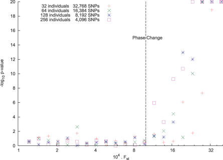
Current methods for inferring population structure from genetic data do not provide formal significance tests for population differentiation. We discuss an approach to studying population structure (principal components analysis) that was first applied to genetic data by Cavalli-Sforza and colleagues. We place the method on a solid statistical footing, using results from modern statistics to develop formal significance tests. We also uncover a general "phase change" phenomenon about the ability to detect structure in genetic data, which emerges from the statistical theory we use, and has an important implication for the ability to discover structure in genetic data: for a fixed but large dataset size, divergence between two populations (as measured, for example, by a statistic like FST) below a threshold is essentially undetectable, but a little above threshold, detection will be easy. This means that we can predict the dataset size needed to detect structure.
Overview
The claims and statistics of this paper haven’t been checked yet.
Free: it reads the open-access text and checks the first 5 claims that cite a source we can check. Create a free account to check every claim.
Integrity signals
Registry
Cites
Statistics
Figures
Verification
Claims the paper makes
The claims and statistics of this paper haven’t been checked yet.
Free: it reads the open-access text and checks the first 5 claims that cite a source we can check. Create a free account to check every claim.
Claims other papers make about this one
Each is checked against this paper’s own text: does it say what the citing paper says it does?
The source backs part of the claim, not all of it — or backs it for a different population, condition or comparison.
In the citing paper
“It is notable that PCA clustering is sensitive to the sample size of different ancestries and also to their amount of genetic drift, which exaggerates principal component distances 207,208,211,212 .”
From Ancient DNA analysis (2021) · cites this paper as [207]
Experimental — accuracy not yet measured
Self-check
Percentages, sums and reported differences re-computed from the paper’s own numbers.
The self-check needs the paper’s full text.
Citations
Cites
Inference of Population Structure Using Multilocus Genotype Data
Pritchard, J. K., Stephens, M., & Donnelly, P. (2000) · Genetics · doi:10.1093/genetics/155.2.945 · Cited by 33,908
Principal components analysis corrects for stratification in genome-wide association studies
Price, A. L., Patterson, N. J., Plenge, R. M., Weinblatt, M. E., Shadick, N. A., & Reich, D. (2006) · Nature Genetics · doi:10.1038/ng1847 · Cited by 10,248 · cited 2×
“A parallel paper [14] explores applications to medical genetics.”
BackgroundSelf-citationFalush, D., Stephens, M., & Pritchard, J. K. (2003) · Genetics · doi:10.1093/genetics/164.4.1567 · Cited by 7,959
The International HapMap Project
†The International HapMap Consortium, Genotyping centres: Baylor College of Medicine and ParAllele BioScience, Gibbs, R. A., Belmont, J. W., Hardenbol, P., Willis, T. D., Yu, F., Chinese HapMap Consortium, Yang, H., Ch'ang, L.-Y., et al. (2003) · Nature · doi:10.1038/nature02168 · Cited by 6,057
A haplotype map of the human genome
The International HapMap Consortium (2005) · Nature · doi:10.1038/nature04226 · Cited by 5,858 · cited 1×
“For instance, in the International Haplotype Map project [ 26 ], markers were chosen about 5,000 bases apart (phase 1), or about 1,000 bases apart (phase 2), and so nearby markers will often be in LD. Mathematically this will induce correlation between nearby columns of our matrix M. The effect of this will be that th…”
BackgroundSpielman, R. S., McGinnis, R. E., & Ewens, W. J. (1993) · PubMed · Cited by 3,651
Searle, S. R., & Searle, S. R. (1971) · Cited by 3,229
The History and Geography of Human Genes: Abridged paperback Edition
Cavalli-Sforza, L. L., Menozzi, P., & Piazza, A. (2018) · Princeton University Press eBooks · doi:10.2307/j.ctv301gjp · Cited by 3,175
Genomic Control for Association Studies
Devlin, B., & Roeder, K. (1999) · Biometrics · doi:10.1111/j.0006-341x.1999.00997.x · Cited by 3,162 · cited 3×
“If e([1]) is the principal eigenvector of the matrix X, this means that the sum of squares”
BackgroundOn the distribution of the largest eigenvalue in principal components analysis
Johnstone, I. M. (2001) · The Annals of Statistics · doi:10.1214/aos/1009210544 · Cited by 1,949 · cited 13×
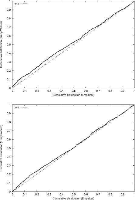
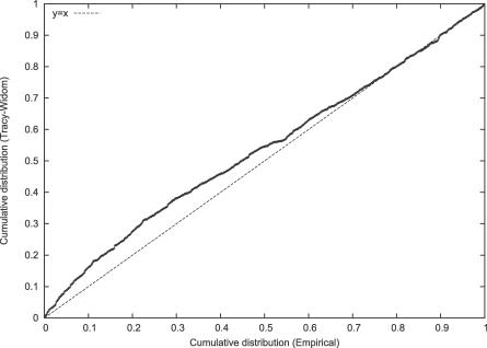
“> λm, then Johnstone [1] shows that with suitable normalization and for large m and n, the largest eigenvalue λ1 is well approximated by the Tracy-Widom distribution.”
BackgroundMethodInfluentialHigh resolution of human evolutionary trees with polymorphic microsatellites
Bowcock, A. M., Ruiz-Linares, A., Tomfohrde, J., Minch, E., Kidd, J. R., & Cavalli-Sforza, L. L. (1994) · Nature · doi:10.1038/368455a0 · Cited by 1,850 · cited 1×
“On the other hand, the individual samples certainly do not have any such construct, and even if population labels are available, initial analysis at an individual level allows us to check the meaningfulness of the labels [20].”
BackgroundLevel-spacing distributions and the Airy kernel
Tracy, C. A., & Widom, H. (1994) · Communications in Mathematical Physics · doi:10.1007/bf02100489 · Cited by 1,828
High-resolution haplotype structure in the human genome
Daly, M. J., Rioux, J. D., Schaffner, S. F., Hudson, T. J., & Lander, E. S. (2001) · Nature Genetics · doi:10.1038/ng1001-229 · Cited by 1,717 · cited 1×
“Suppose, for example, that there is a large ‘‘block’’ [35,36] in which markers are in complete LD, and we have genotyped many markers in the block.”
BackgroundHistory and Geography of Human Genes
Piazza, A. (1994) · Advances in Forensic Haemogenetics · doi:10.1007/978-3-642-78782-9_1 · Cited by 1,639
The history and geography of human genes
(1995) · Choice Reviews Online · doi:10.5860/choice.33-0316 · Cited by 1,312
ON THE RELATIVE ABUNDANCE OF BIRD SPECIES
MacArthur, R. H. (1957) · Proceedings of the National Academy of Sciences · doi:10.1073/pnas.43.3.293 · Cited by 1,172 · cited 2×
“One technique is the ‘‘broken stick’’ model [27,28], used, for instance, in a recent population genetics analysis [5].”
BackgroundMethodBlocks of Limited Haplotype Diversity Revealed by High-Resolution Scanning of Human Chromosome 21
Patil, N., Berno, A. J., Hinds, D. A., Barrett, W. A., Doshi, J. M., Hacker, C. R., Kautzer, C. R., Lee, D. H., Marjoribanks, C., McDonough, D. P., et al. (2001) · Science · doi:10.1126/science.1065573 · Cited by 1,145
Ramachandran, S., Deshpande, O., Roseman, C. C., Rosenberg, N. A., Feldman, M. W., & Cavalli-Sforza, L. L. (2005) · Proceedings of the National Academy of Sciences · doi:10.1073/pnas.0507611102 · Cited by 1,103 · cited 3×
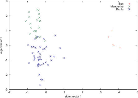
“Plots of the first two eigenvectors for some African populations in the CEPH–HGDP dataset [30].”
BackgroundMethodPhase transition of the largest eigenvalue for nonnull complex sample covariance matrices
Baik, J., Ben Arous, G., & Péché, S. (2005) · The Annals of Probability · doi:10.1214/009117905000000233 · Cited by 967 · cited 8×
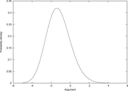
“The phase change effect was suggested by a recent paper in theoretical statistics [16], which demonstrated the phenomenon for a situation that is mathematically similar to ours.”
BackgroundResultInfluentialThe effects of human population structure on large genetic association studies
Marchini, J., Cardon, L. R., Phillips, M. S., & Donnelly, P. (2004) · Nature Genetics · doi:10.1038/ng1337 · Cited by 869 · cited 1×
“We believe they will prove useful both in medical genetics, where population structure may cause spurious disease associations [1,40–43]; and in population genetics, where our statistical methods provide a strong indication of how many axes of variation are meaningful.”
BackgroundAssessing the impact of population stratification on genetic association studies
Freedman, M. L., Reich, D., Penney, K. L., McDonald, G. J., Mignault, A. A., Patterson, N., Gabriel, S. B., Topol, E. J., Smoller, J. W., Pato, C. N., et al. (2004) · Nature Genetics · doi:10.1038/ng1333 · Cited by 806 · cited 1×
“We believe they will prove useful both in medical genetics, where population structure may cause spurious disease associations [1,40–43]; and in population genetics, where our statistical methods provide a strong indication of how many axes of variation are meaningful.”
BackgroundSelf-citationMatrix Computations, 3rd Edition
Golub, G. H. (2007) · Cited by 787
Eigenvalues of large sample covariance matrices of spiked population models
Baik, J., & Silverstein, J. W. (2006) · Journal of Multivariate Analysis · doi:10.1016/j.jmva.2005.08.003 · Cited by 701 · cited 2×
“The theory has continued to develop and nearly all we need has now been proved, the most recent paper being [17].”
BackgroundThe application of molecular genetic approaches to the study of human evolution
Cavalli-Sforza, L. L., & Feldman, M. W. (2003) · Nature Genetics · doi:10.1038/ng1113 · Cited by 676 · cited 1×
“In population genetics, we recommend a review paper [3] focusing on the use of ‘‘synthetic maps’’ which use PCA to study genetic geographic variation.”
MethodMenozzi, P., Piazza, A., & Cavalli-Sforza, L. (1978) · Science · doi:10.1126/science.356262 · Cited by 638 · cited 9×
“Based on these results, we are able to give an estimate of how much data will be required to find population structure given a level of genetic divergence such as FST (as defined by Cavalli-Sforza, [15, p. 26, Equation 3].)”
BackgroundMethodInfluentialCalibrating a coalescent simulation of human genome sequence variation
Schaffner, S. F., Foo, C., Gabriel, S., Reich, D., Daly, M. J., & Altshuler, D. (2005) · Genome Research · doi:10.1101/gr.3709305 · Cited by 616 · cited 1×
“We thank Stephen Schaffner for sharing a powerful and flexible coalescent simulator [46] which was helpful for many of our simulations, and Mira Bernstein for catching an important error.”
MethodSelf-citationGould, A. L. (1973) · Technometrics · doi:10.1080/00401706.1973.10489027 · Cited by 579
Clines, Clusters, and the Effect of Study Design on the Inference of Human Population Structure
Rosenberg, N. A., Mahajan, S., Ramachandran, S., Zhao, C., Pritchard, J. K., & Feldman, M. W. (2005) · PLoS Genetics · doi:10.1371/journal.pgen.0010070 · Cited by 568
Clayton, D. G., Walker, N. M., Smyth, D. J., Pask, R., Cooper, J. D., Maier, L. M., Smink, L. J., Lam, A. C., Ovington, N. R., Stevens, H. E., et al. (2005) · Nature Genetics · doi:10.1038/ng1653 · Cited by 526 · cited 2×
“This is discussed in detail in [38], which is”
BackgroundBalding, D. J., & Nichols, R. A. (1995) · Genetica · doi:10.1007/bf01441146 · Cited by 503 · cited 6×
“We note that Nicholson et al. use the same normalization, and motivate it similarly [18].”
MethodInfluentialMethods for High-Density Admixture Mapping of Disease Genes
Patterson, N., Hattangadi, N., Lane, B., Lohmueller, K. E., Hafler, D. A., Oksenberg, J. R., Hauser, S. L., Smith, M. W., O’Brien, S. J., Altshuler, D., et al. (2004) · The American Journal of Human Genetics · doi:10.1086/420871 · Cited by 478 · cited 5×
“Indeed, on this dataset the correlation of our principal eigenvector with the estimated European ancestry for each individual recovered by the admixture analysis program ANCESTRYMAP [12] is a remarkable .995 (STRUCTURE produces similar results).”
BackgroundMethodInfluentialSelf-citationA High-Density Admixture Map for Disease Gene Discovery in African Americans
Smith, M. W., Patterson, N., Lautenberger, J. A., Truelove, A. L., McDonald, G. J., Waliszewska, A., Kessing, B. D., Malasky, M. J., Scafe, C., Le, E., et al. (2004) · The American Journal of Human Genetics · doi:10.1086/420856 · Cited by 459 · cited 1×
“We attempted to apply our methods to an African-American dataset genotyped on a panel of ancestryinformative markers [ 34 ].”
MethodSelf-citationThompson, W. A. (1963) · Technometrics · doi:10.1080/00401706.1963.10490115 · Cited by 455
Evidence for Gradients of Human Genetic Diversity Within and Among Continents
Serre, D., & Pääbo, S. (2004) · Genome Research · doi:10.1101/gr.2529604 · Cited by 436 · cited 1×
“As pointed out in [39], the sampling strategy can affect the apparent structure.”
BackgroundAlu Insertion Polymorphisms and Human Evolution: Evidence for a Larger Population Size in Africa
Stoneking, M., Fontius, J. J., Clifford, S. L., Soodyall, H., Arcot, S. S., Saha, N., Jenkins, T., Tahir, M. A., Deininger, P. L., & Batzer, M. A. (1997) · Genome Research · doi:10.1101/gr.7.11.1061 · Cited by 346 · cited 1×
“In addition to single nucleotide polymorphisms (SNPs) and microsatellites, PCA has been applied to haplotype frequencies [6,7] and the distribution of ALU insertion polymorphisms [8] in order to study population structure.”
MethodDesign and Analysis of Admixture Mapping Studies
Hoggart, C. J., Shriver, M. D., Kittles, R. A., Clayton, D. G., & McKeigue, P. M. (2004) · The American Journal of Human Genetics · doi:10.1086/420855 · Cited by 304 · cited 2×
“) Finally, if ‘‘admixture LD’’ is present, so that in admixed individuals long segments of the genome originate from one founder population, simple PCA methods will not be as powerful as programs such as STRUCTURE [10], ADMIXMAP [11], and ANCESTRYMAP [12], where there is careful modeling of the admixture blocks and th…”
MethodAn Icelandic example of the impact of population structure on association studies
Helgason, A., Yngvadóttir, B., Hrafnkelsson, B., Gulcher, J., & Stefánsson, K. (2005) · Nature Genetics · doi:10.1038/ng1492 · Cited by 285 · cited 1×
“We believe they will prove useful both in medical genetics, where population structure may cause spurious disease associations [1,40–43]; and in population genetics, where our statistical methods provide a strong indication of how many axes of variation are meaningful.”
BackgroundRosenberg, N. A. (2006) · Annals of Human Genetics · doi:10.1111/j.1469-1809.2006.00285.x · Cited by 246 · cited 1×
“For the data used in Figure 4, we use the H952 subset of the CEPH–HGDP panel [30,31,45] where some atypical samples and pairs of close relatives have been removed.”
MethodSoshnikov, A. (2002) · Journal of Statistical Physics · doi:10.1023/a:1019739414239 · Cited by 227
Assessing Population Differentiation and Isolation from Single-Nucleotide Polymorphism Data
Nicholson, G., Smith, A. V., Jónsson, F., Gústafsson, Ó., Stefánsson, K., & Donnelly, P. (2002) · Journal of the Royal Statistical Society Series B: Statistical Methodology · doi:10.1111/1467-9868.00357 · Cited by 223 · cited 3×
“[18], and STRUCTURE [9] in the correlated allele mode.”
BackgroundMethodChakraborty, R., & Jin, L. (1993) · DNA Fingerprinting: State of the Science · doi:10.1007/978-3-0348-8583-6_14 · Cited by 221
Statistical Tests for Admixture Mapping with Case-Control and Cases-Only Data
Montana, G., & Pritchard, J. K. (2004) · The American Journal of Human Genetics · doi:10.1086/425281 · Cited by 160 · cited 1×
“In complex situations, such as uncovering structure in populations where all individuals are equal mixtures of ancestral populations, it may remain necessary to use statistical software that explicitly models admixture LD, such as [10–13], which allow estimation of local ancestry at arbitrary points of the genome.”
MethodLarge-scale SNP analysis reveals clustered and continuous patterns of human genetic variation
Shriver, M. D., Mei, R., Parra, E. J., Sonpar, V. A., Halder, I., Tishkoff, S. A., Schurr, T. G., Zhadanov, S. I., Osipova, L. P., Brutsaert, T. D., et al. (2005) · Human Genomics · doi:10.1186/1479-7364-2-2-81 · Cited by 150 · cited 5×
“For the data of Mark Shriver and colleagues [5], we analyzed only autosomal data where no SNP had any missing data.”
BackgroundMethodInfluentialKaroui, N. E. (2003) · arXiv (Cornell University) · doi:10.48550/arxiv.math/0309355 · Cited by 96
Population Structure in the Mediterranean Basin: A Y Chromosome Perspective
Capelli, C., Redhead, N., Romano, V., Calì, F., Lefranc, G., Delague, V., Mégarbané, A., Felice, A. E., Pascali, V. L., Neophytou, P. I., et al. (2005) · Annals of Human Genetics · doi:10.1111/j.1529-8817.2005.00224.x · Cited by 83 · cited 1×
“In addition to single nucleotide polymorphisms (SNPs) and microsatellites, PCA has been applied to haplotype frequencies [6,7] and the distribution of ALU insertion polymorphisms [8] in order to study population structure.”
MethodInformative Missingness in Genetic Association Studies: Case-Parent Designs
Allen, A. S., Rathouz, P. J., & Satten, G. A. (2003) · The American Journal of Human Genetics · doi:10.1086/368276 · Cited by 66 · cited 1×
“’’ Unfortunately ‘‘informative missingness’’ [37,38] is”
Shin, J.-H., Janer, M., McNeney, B., Blay, S., Deutsch, K., SANJEEVI, C. B., Kockum, I. S., Lernmark, Å., Graham, J., & Groups, O. B. O. T. S. C. D. A. T. D. I. I. S. S. (2007) · Genes and Immunity · doi:10.1038/sj.gene.6364413 · Cited by 47
Ethiopia: between Sub-Saharan Africa and western Eurasia.
Lovell, A. D., Moreau, C., Yotova, V., Xiao, F., Bourgeois, S., Gehl, D., Bertranpetit, J., Schurr, E., & Labuda, D. (2005) · Annals of Human Genetics · doi:10.1046/j.1529-8817.2005.00152.x · Cited by 37 · cited 1×
“In addition to single nucleotide polymorphisms (SNPs) and microsatellites, PCA has been applied to haplotype frequencies [6,7] and the distribution of ALU insertion polymorphisms [8] in order to study population structure.”
MethodEthiopia: between Sub‐Saharan Africa and Western Eurasia
Lovell, A. D., Moreau, C., Yotova, V., Xiao, F., Bourgeois, S., Gehl, D., Bertranpetit, J., Schurr, E., & Labuda, D. (2005) · doi:10.1046/j.1469-1809.2005.00152.x · Cited by 22
Research works printed but not linked: 39
- Devlin, 1999, Biometrics, 55, 997
- Menozzi, 1978, Science, 201, 786
- Cavalli-Sforza, 2003, Nat Genet, 33, 266
- Shriver, 2005, Human Genomics, 2, 81
- Capelli, 2006, Ann Hum Genet, 70, 207
- Lovell, 2005, Ann Hum Genet, 69, 275
- Stoneking, 1997, Genome Res, 7, 1061
- Pritchard, 2000, Genetics, 155, 945
- Falush, 2003, Genetics, 164, 1567
- Hoggart, 2004, Am J Hum Genet, 74, 965
- Patterson, 2004, Am J Hum Genet, 74, 979
- Montana, 2004, Am J Hum Genet, 75, 771
- Price, 2006, Nat Genet, 38, 904
- Baik, 2005, Ann Probability, 33, 1643
- Baik, 2006, J Multivariate Anal, 97, 1643
- Nicholson, 2002, JRSS(B), 64, 695
- Bowcock, 1994, Nature, 368, 455
- Johnstone, 2001, Ann Stat, 29, 295
- Tracy, 1994, Commun Math Phys, 159, 151
- El Karoui, 2003, On the largest eigenvalue of Wishart matrices with identity covariance when p/n → ∞
- Soshnikov, 2002, J Stat Physics, 108, 1033
- Altshuler, 2005, Nature, 437, 1299
- Macarthur, 1957, Proc Natl Acad Sci U S A, 43, 293
- Pielou, 1975, Ecological diversity
- Ramachandran, 2005, Proc Natl Acad Sci, 102, 15942
- Gibbs, 2004, Nature, 426, 789
- Smith, 2004, Am J Hum Genet, 74, 1001
- Daly, 2001, Nat Genet, 29, 229
- Patil, 2001, Science, 294, 1719
- Allen, 2003, Am J Hum Genet, 72, 671
- Clayton, 2005, Nat Genet, 37, 1243
- Serre, 2004, Genome Res, 14, 1679
- Spielman, 1993, Am J Hum Genet, 52, 506
- Freedman, 2004, Nat Genet, 36, 388
- Marchini, 2004, Nat Genet, 36, 512
- Helgason, 2005, Nat Genet, 37, 90
- Balding, 1995, Genetica, 96, 3
- Rosenberg, 2006, Ann Hum Gen, 70, 841
- Schaffner, 2005, Genome Res, 15, 1576
Cited by
Two new Later Stone Age sites from the Final Pleistocene in the Falémé Valley, eastern Senegal
Ndiaye, M., Lespez, L., Tribolo, C., Rassé, M., Hadjas, I., Davidoux, S., Huysecom, É., & Douze, K. (2024) · Monash University Research Portal (Monash University) · doi:10.3929/ethz-b-000667478 · Cited by 23,868
Fast model-based estimation of ancestry in unrelated individuals
Alexander, D. H., Novembre, J., & Lange, K. (2009) · Genome Research · doi:10.1101/gr.094052.109 · Cited by 9,898
“EIGENSTRAT (Patterson et al. 2006; Price et al. 2006) is a popular implementation of PCA for ancestry inference.”
MethodLD Score regression distinguishes confounding from polygenicity in genome-wide association studies
Schizophrenia Working Group of the Psychiatric Genomics Consortium, Bulik-Sullivan, B. K., Loh, P.-R., Finucane, H. K., Ripke, S., Yang, J., Patterson, N., Daly, M. J., Price, A. L., & Neale, B. M. (2015) · Nature Genetics · doi:10.1038/ng.3211 · Cited by 5,559
Self-citationJombart, T., Devillard, S., & Balloux, F. (2010) · BMC Genetics · doi:10.1186/1471-2156-11-94 · Cited by 4,963
“Multivariate analyses have been used for decades to extract various types of information from genetic data and have attracted renewed interest in the field [ 6-12 ].”
Common SNPs explain a large proportion of the heritability for human height
Yang, J., Benyamin, B., McEvoy, B. P., Gordon, S., Henders, A. K., Nyholt, D. R., Madden, P. A., Heath, A. C., Martin, N. G., Montgomery, G. W., et al. (2010) · Nature Genetics · doi:10.1038/ng.608 · Cited by 4,446
Metadata
- Authors
- Patterson, N., Price, A. L., & Reich, D.
- Affiliations
- Broad Institute (US)
- Corresponding author
- Patterson, Nick
- Venue
- PLoS Genetics
- Publisher
- Public Library of Science (PLoS)
- Published
- 2006
- Volume
- 2
- Issue
- 12
- Pages
- e190
- ISSN
- 1553-7390 (ISSN-L)
- 1553-7404
- PMC
- PMC1713260
- OpenAlex
- W2108169091
- Cited by
- 5,280
- References
- 49
- Citations by year
- 2026: 303 · 2025: 380 · 2024: 430 · 2023: 361 · 2022: 393 · 2021: 405 · 2020: 352 · 2019: 324 · 2018: 313 · 2017: 298 · 2016: 270 · 2015: 250 · 2014: 248 · 2013: 227 · 2012: 212
- FWCI
- 35.78
- Type
- journal article
- Language
- en
- Open access
- gold
- doi.org
- Locations
- PLoS Genetics (publishedVersion, cc-by)
- Europe PMC (PubMed Central) (publishedVersion, cc-by)
- PubMed Central (publishedVersion, cc-by)
- PubMed (publishedVersion)
- Digital Access to Scholarship at Harvard (DASH) (Harvard University) (submittedVersion, cc-by)
- RePEc: Research Papers in Economics (submittedVersion)
- DOAJ (DOAJ: Directory of Open Access Journals) (submittedVersion)
- Funders
- Wellcome Trust
- National Human Genome Research Institute (R01HG006399)
- Topics
- Life Sciences › Biochemistry, Genetics and Molecular Biology › Genetics › Genetic diversity and population structure
- Life Sciences › Biochemistry, Genetics and Molecular Biology › Genetics › Forensic and Genetic Research
- Life Sciences › Biochemistry, Genetics and Molecular Biology › Genetics › Genetic Associations and Epidemiology
- Keywords
- population structure, principal component analysis, significance tests, genetic differentiation, phase transitions, sample size determination, FST, genetic data, eigenvalue analysis
- MeSH terms
- Computer Simulation, Genetic Markers, Genetics, Medical, Genetics, Population, Humans, Models, Genetic, Genetic Variation, Models, Statistical, Principal Component Analysis
About these checks
Registry, retraction, Cites and statistics results are computed, not judged, with one exception: a printed reference that no index lists is read once by a model before it counts as a citation error. Claims are extracted by a model and kept only when their quote appears verbatim in the text; each cited source is then checked, with a model’s help, for whether it says what the claim relies on. Those verdicts can be wrong — read the claim’s quote and the cited source before relying on one.
Statistics and arithmetic are recomputed, not judged.
Confidence bands are shown only for fields calibrated on our annotated test set. None is calibrated yet, so no band is shown.
What counts as a claim ›How we measure confidence ›How we check this ›
Are you an author, or do you see a problem with this page? Request a review
Data sources
Bibliographic data: Semantic Scholar, OpenAlex, Crossref.
Contains information from the Semantic Scholar Academic Graph Datasets, made available under the ODC Attribution License (ODC-BY 1.0).
Semantic Scholar’s data is described in: Kinney, R., et al. (2023). The Semantic Scholar Open Data Platform. arXiv:2301.10140.
