

The DOI matches its Crossref record; 7 of the 7 references it cites were found in a registry or an index.
Fine-mapping from summary data with the “Sum of Single Effects” model
Open accessPublished version of a preprint
Abstract
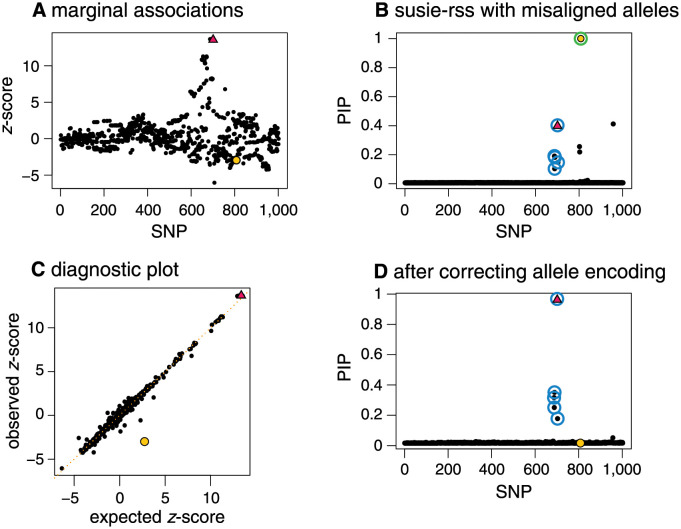
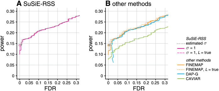
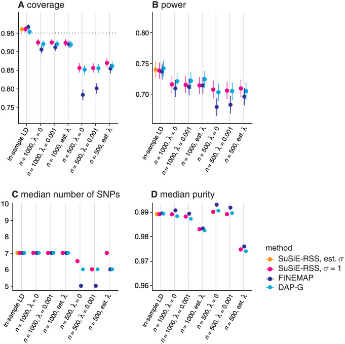
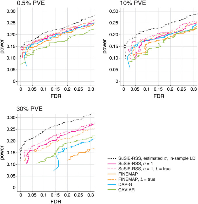
In recent work, Wang et al introduced the “Sum of Single Effects” ( SuSiE ) model, and showed that it provides a simple and efficient approach to fine-mapping genetic variants from individual-level data. Here we present new methods for fitting the SuSiE model to summary data, for example to single-SNP z -scores from an association study and linkage disequilibrium (LD) values estimated from a suitable reference panel. To develop these new methods, we first describe a simple, generic strategy for extending any individual-level data method to deal with summary data. The key idea is to replace the usual regression likelihood with an analogous likelihood based on summary data. We show that existing fine-mapping methods such as FINEMAP and CAVIAR also (implicitly) use this strategy, but in different ways, and so this provides a common framework for understanding different methods for fine-mapping. We investigate other common practical issues in fine-mapping with summary data, including problems caused by inconsistencies between the z -scores and LD estimates, and we develop diagnostics to identify these inconsistencies. We also present a new refinement procedure that improves model fits in some data sets, and hence improves overall reliability of the SuSiE fine-mapping results. Detailed evaluations of fine-mapping methods in a range of simulated data sets show that SuSiE applied to summary data is competitive, in both speed and accuracy, with the best available fine-mapping methods for summary data.
Overview
The claims and statistics of this paper haven’t been checked yet.
Run the check — free, no account needed. It reads the open-access text and checks the sources it cites.
Integrity signals
Registry
Cites
Statistics
Figures


Verification
Claims the paper makes
The claims and statistics of this paper haven’t been checked yet.
Run the check — free, no account needed. It reads the open-access text and checks the sources it cites.
Claims other papers make about this one
Each is checked against this paper’s own text: does it say what the citing paper says it does?
The source backs part of the claim, not all of it — or backs it for a different population, condition or comparison.
In the citing paper
“The s values from SuSiE-RSS ranged from 0.007 to 0.027 across fine-mapped loci, and the diagnostic plots demonstrated high consistency of LD between the summary statistics and reference panel (Supplementary Fig. 19a–g).”
From Shared genetic architectures of educational attainment in East Asian and European populations (2024) · cites this paper as [34]
Experimental — accuracy not yet measured
Self-check
Percentages, sums and reported differences re-computed from the paper’s own numbers.
The self-check needs the paper’s full text.
Citations
Cites
Second-generation PLINK: rising to the challenge of larger and richer datasets
Chang, C. C., Chow, C. C., Tellier, L. C., Vattikuti, S., Purcell, S. M., & Lee, J. J. (2015) · Gigascience · doi:10.1186/s13742-015-0047-8 · Cited by 12,709
METAL: fast and efficient meta-analysis of genomewide association scans
Willer, C. J., Li, Y., & Abecasis, G. R. (2010) · Bioinformatics · doi:10.1093/bioinformatics/btq340 · Cited by 5,205
The Genotype-Tissue Expression (GTEx) pilot analysis: Multitissue gene regulation in humans
The GTEx Consortium, Ardlie, K. G., Deluca, D. S., Segrè, A. V., Sullivan, T. J., Young, T. R., Gelfand, E. T., Trowbridge, C. A., Maller, J. B., Tukiainen, T., et al. (2015) · Science · doi:10.1126/science.1262110 · Cited by 5,062
Self-citationGiambartolomei, C., Vukcevic, D., Schadt, E. E., Franke, L., Hingorani, A. D., Wallace, C., & Plagnol, V. (2014) · PLoS Genetics · doi:10.1371/journal.pgen.1004383 · Cited by 4,261
A well-conditioned estimator for large-dimensional covariance matrices
Ledoit, O., & Wolf, M. (2004) · Journal of Multivariate Analysis · doi:10.1016/s0047-259x(03)00096-4 · Cited by 3,046 · cited 1×
“A common way to improve estimation of covariance matrices is to use regularization [38], replacing R̂ with R̂l, R̂l ≔ ð1 lÞR̂0 þ lI; ð23Þ”
Genetic Investigation of ANthropometric Traits (GIANT) Consortium, Yang, J., DIAbetes Genetics Replication And Meta-analysis (DIAGRAM) Consortium, Ferreira, T., Morris, A. P., Medland, S. E., Madden, P. A. F., Heath, A. C., Martin, N. G., Montgomery, G. W., et al. (2012) · Nature Genetics · doi:10.1038/ng.2213 · Cited by 1,712
High-Resolution Mapping of Expression-QTLs Yields Insight into Human Gene Regulation
Veyrieras, J.-B., Kudaravalli, S., Kim, S. Y., Dermitzakis, E. T., Gilad, Y., Stephens, M., & Pritchard, J. K. (2008) · PLoS Genetics · doi:10.1371/journal.pgen.1000214 · Cited by 536
Self-citation
Research works printed but not linked: 45
- A Hutchinson, 2020, Fine-mapping genetic associations, Human Molecular Genetics, 29, R81, 10.1093/hmg/ddaa148 · DOI
- JB Maller, 2012, Bayesian refinement of association signals for 14 loci in 3 common diseases, Nature Genetics, 44, 1294, 10.1038/ng.2435 · DOI
- Z Kote-Jarai, 2013, Fine-mapping identifies multiple prostate cancer risk loci at 5p15, one of which associates with TERT expression, Human Molecular Genetics, 22, 2520, 10.1093/hmg/ddt086 · DOI
- DJ Schaid, 2018, From genome-wide associations to candidate causal variants by statistical fine-mapping, Nature Reviews Genetics, 19, 491, 10.1038/s41576-018-0016-z · DOI
- SL Spain, 2015, Strategies for fine-mapping complex traits, Human Molecular Genetics, 24, R111, 10.1093/hmg/ddv260 · DOI
- PM Visscher, 2017, 10 years of GWAS discovery: biology, function, and translation, American Journal of Human Genetics, 101, 5, 10.1016/j.ajhg.2017.06.005 · DOI · Paper page
- F Hormozdiari, 2014, Identifying causal variants at loci with multiple signals of association, Genetics, 198, 497, 10.1534/genetics.114.167908 · DOI · Paper page
- G Kichaev, 2014, Integrating functional data to prioritize causal variants in statistical fine-mapping studies, PLoS Genetics, 10, e1004722, 10.1371/journal.pgen.1004722 · DOI
- B Servin, 2007, Imputation-based analysis of association studies: candidate regions and quantitative traits, PLoS Genetics, 3, e114, 10.1371/journal.pgen.0030114 · DOI
- W Chen, 2015, Fine mapping causal variants with an approximate Bayesian method using marginal test statistics, Genetics, 200, 719, 10.1534/genetics.115.176107 · DOI
- C Benner, 2016, FINEMAP: efficient variable selection using summary data from genome-wide association studies, Bioinformatics, 32, 1493, 10.1093/bioinformatics/btw018 · DOI · Paper page
- Y Li, 2016, Joint Bayesian inference of risk variants and tissue-specific epigenomic enrichments across multiple complex human diseases, Nucleic Acids Research, 44, e144, 10.1093/nar/gkw627 · DOI
- X Wen, 2016, Efficient integrative multi-SNP association analysis via deterministic approximation of posteriors, American Journal of Human Genetics, 98, 1114, 10.1016/j.ajhg.2016.03.029 · DOI
- PJ Newcombe, 2016, JAM: a scalable Bayesian framework for joint analysis of marginal SNP effects, Genetic Epidemiology, 40, 188, 10.1002/gepi.21953 · DOI
- Y Lee, 2018, Bayesian multi-SNP genetic association analysis: control of FDR and use of summary statistics, bioRxiv
- G Wang, 2020, A simple new approach to variable selection in regression, with application to genetic fine mapping, Journal of the Royal Statistical Society, Series B, 82, 1273, 10.1111/rssb.12388 · DOI · Paper page
- M Sesia, 2020, Multi-resolution localization of causal variants across the genome, Nature Communications, 11, 1093, 10.1038/s41467-020-14791-2 · DOI
- C Wallace, 2015, Dissection of a complex disease susceptibility region using a Bayesian stochastic search approach to fine mapping, PLoS Genetics, 11, e1005272, 10.1371/journal.pgen.1005272 · DOI
- A Hutchinson, 2020, Improving the coverage of credible sets in Bayesian genetic fine-mapping, PLoS Computational Biology, 16, e1007829, 10.1371/journal.pcbi.1007829 · DOI
- C Benner, 2018, Refining fine-mapping: effect sizes and regional heritability, bioRxiv
- B Pasaniuc, 2017, Dissecting the genetics of complex traits using summary association statistics, Nature Reviews Genetics, 18, 117, 10.1038/nrg.2016.142 · DOI
- X Zhu, 2017, Bayesian large-scale multiple regression with summary statistics from genome-wide association studies, Annals of Applied Statistics, 11, 1561
- analysis Initiative GBM, 2022, Meta-analysis fine-mapping is often miscalibrated at single-variant resolution, medRxiv
- Chipman H, George EI, McCulloch RE. The practical implementation of Bayesian model selection. In: Model Selection. vol. 38 of IMS Lecture Notes. Institute of Mathematical Statistics; 2001. p. 65–116. · DOI · Paper page
- JK Pickrell, 2014, Joint analysis of functional genomic data and genome-wide association studies of 18 human traits, American Journal of Human Genetics, 94, 559, 10.1016/j.ajhg.2014.03.004 · DOI
- C Benner, 2017, Prospects of fine-mapping trait-associated genomic regions by using summary statistics from genome-wide association studies, American Journal of Human Genetics, 101, 539, 10.1016/j.ajhg.2017.08.012 · DOI
- M Stephens, 2009, Bayesian statistical methods for genetic association studies, Nature Reviews Genetics, 10, 681, 10.1038/nrg2615 · DOI
- J Wakefield, 2009, Bayes factors for genome-wide association studies: comparison with P-values, Genetic Epidemiology, 33, 79, 10.1002/gepi.20359 · DOI
- Y Zou, 2021, Fine-mapping from summary data with the “Sum of Single Effects” model, bioRxiv
- JA Lozano, 2017, The multivariate normal distribution framework for analyzing association studies, bioRxiv
- Y Park, 2017, A Bayesian approach to mediation analysis predicts 206 causal target genes in Alzheimer’s disease, bioRxiv
- TSH Mak, 2017, Polygenic scores via penalized regression on summary statistics, Genetic Epidemiology, 41, 469, 10.1002/gepi.22050 · DOI
- B Pasaniuc, 2014, Fast and accurate imputation of summary statistics enhances evidence of functional enrichment, Bioinformatics, 30, 2906, 10.1093/bioinformatics/btu416 · DOI
- W Chen, 2021, Improved analyses of GWAS summary statistics by reducing data heterogeneity and errors, Nature Communications, 12, 7117, 10.1038/s41467-021-27438-7 · DOI
- D Lee, 2013, DIST: direct imputation of summary statistics for unmeasured SNPs, Bioinformatics, 29, 2925, 10.1093/bioinformatics/btt500 · DOI
- N LaPierre, 2020, Identifying causal variants by fine mapping across multiple studies, bioRxiv
- C Bycroft, 2018, The UK Biobank resource with deep phenotyping and genomic data, Nature, 562, 203, 10.1038/s41586-018-0579-z · DOI · Paper page
- Y Guan, 2011, Bayesian variable selection regression for genome-wide association studies and other large-scale problems, Annals of Applied Statistics, 5, 1780, 10.1214/11-AOAS455 · DOI
- W Bodmer, 2008, Common and rare variants in multifactorial susceptibility to common diseases, Nature Genetics, 40, 695, 10.1038/ng.f.136 · DOI · Paper page
- JPA Ioannidis, 2006, Implications of small effect sizes of individual genetic variants on the design and interpretation of genetic association studies of complex diseases, American Journal of Epidemiology, 164, 609, 10.1093/aje/kwj259 · DOI
- AN Barbeira, 2021, Exploiting the GTEx resources to decipher the mechanisms at GWAS loci, Genome Biology, 22, 49, 10.1186/s13059-020-02252-4 · DOI
- X Wen, 2015, Cross-population joint analysis of eQTLs: fine mapping and functional annotation, PLoS Genetics, 11, e1005176, 10.1371/journal.pgen.1005176 · DOI
- Z Zhu, 2016, Integration of summary data from GWAS and eQTL studies predicts complex trait gene targets, Nature Genetics, 48, 481, 10.1038/ng.3538 · DOI · Paper page
- B Han, 2009, Rapid and accurate multiple testing correction and power estimation for millions of correlated markers, PLoS Genetics, 5, e1000456, 10.1371/journal.pgen.1000456 · DOI
- M Pirinen, 2013, Efficient computation with a linear mixed model on large-scale data sets with applications to genetic studies, Annals of Applied Statistics, 7, 369, 10.1214/12-AOAS586 · DOI
Cited by
Sorted by citations
Diversity and scale: Genetic architecture of 2068 traits in the VA Million Veteran Program
Verma, A., Huffman, J. E., Rodriguez, A., Conery, M., Liu, M., Ho, Y.-L., Kim, Y., Heise, D. A., Guare, L., Panickan, V. A., et al. (2024) · Science · doi:10.1126/science.adj1182 · Cited by 463
“…of putative causal genetic variants that could be qualitatively and quantitatively compared across population groups, we performed within-population group fine-mapping using the Sum of Single Effects model implemented in SuSiE ( 18 , 19 ) followed by multipopulation credible set integration.”
Zuber, V., Grinberg, N. F., Gill, D., Manipur, I., Slob, E. A. W., Patel, A., Wallace, C., & Burgess, S. (2022) · The American Journal of Human Genetics · doi:10.1016/j.ajhg.2022.04.001 · Cited by 532
Nievergelt, C. M., Maihofer, A. X., Atkinson, E. G., Chen, C., Choi, K. W., Coleman, J. R. I., Daskalakis, N. P., Duncan, L. E., Polimanti, R. A., Aaronson, C. J., et al. (2024) · Nature Genetics · doi:10.1038/s41588-024-01707-9 · Cited by 234
“The SUSIE model assumed a maximum of two causal variants.”
InfluentialKarollus, A., Mauermeier, T., & Gagneur, J. (2023) · Genome Biology · doi:10.1186/s13059-023-02899-9 · Cited by 128
“A fine-mapping method was applied to associate each eQTL with a credible set of likely-causal variants and account for linkage (SuSie [25,26]).”
MethodA disease-associated gene desert directs macrophage inflammation through ETS2
Stankey, C. T., Bourges, C., Haag, L.-M., Turner‐Stokes, T., Piedade, A. P., Palmer-Jones, C., Papa, I., dos Santos, M. S., Zhang, Q., Cameron, A. J., et al. (2024) · Nature · doi:10.1038/s41586-024-07501-1 · Cited by 163
“IBD GWAS summary statistics 3 were used to perform multiple causal variant fine-mapping using susieR 51 , with reference minor allele and LD information calculated from 503 European samples from 1000 Genomes phase 3 (ref.”
MethodTranslational genomics of osteoarthritis in 1,962,069 individuals
Hatzikotoulas, K., Southam, L., Stefánsdóttir, L., Boer, C. G., McDonald, M., Pett, J. P., Park, Y., Tuerlings, M., Mulders, R., Barysenka, A., et al. (2025) · Nature · doi:10.1038/s41586-025-08771-z · Cited by 99
Systems biology dissection of PTSD and MDD across brain regions, cell types, and blood
Daskalakis, N. P., Iatrou, A., Chatzinakos, C., Jajoo, A., Snijders, C., Wylie, D., DiPietro, C. P., Tsatsani, I., Chen, C.-Y., Pernia, C. D., et al. (2024) · Science · doi:10.1126/science.adh3707 · Cited by 109
“For fine mapping,weusedacombinationofFUMA( 77 )with SusieR ( 78 , 79 ).”
Identifying and correcting for misspecifications in GWAS summary statistics and polygenic scores
Privé, F., Arbel, J., Aschard, H., & Vilhjálmsson, B. J. (2022) · Human Genetics and Genomics Advances · doi:10.1016/j.xhgg.2022.100136 · Cited by 85
“identifying false-positives in finemapping (Zou et al., 2021) Quality control”
Sterenborg, R. B. T. M., Steinbrenner, I., Li, Y., Bujnis, M. N., Naito, T., Marouli, E., Galesloot, T. E., Babajide, O., Andreasen, L., Astrup, A., et al. (2024) · Nature Communications · doi:10.1038/s41467-024-44701-9 · Cited by 79
Sources of gene expression variation in a globally diverse human cohort
Taylor, D. J., Chhetri, S. B., Tassia, M. G., Biddanda, A., Yan, S. M., Wojcik, G. L., Battle, A. J., & McCoy, R. C. (2024) · Nature · doi:10.1038/s41586-024-07708-2 · Cited by 83
Genetic regulation of gene expression across multiple tissues in chickens
Guan, D., Bai, Z., Zhu, X., Zhong, C., Hou, Y., Zhu, D., Li, H., Lan, F., Diao, S., Yao, Y., et al. (2025) · Nature Genetics · doi:10.1038/s41588-025-02155-9 · Cited by 99
“Secondly, we fine-mapped putative causal variants for each molecular phenotype by using the “Sum of Single Effects” (SuSiE) model (v.1.0) 92 .”
InfluentialZhao, S., Crouse, W. L., Qian, S., Luo, K., Stephens, M., & He, X. (2024) · Nature Genetics · doi:10.1038/s41588-023-01648-9 · Cited by 79
“For each block with maximum gene PIP > 0.8, we rerun SuSiE-RSS with L = 5 with the original SNPs to get the final gene PIPs.”
InfluentialSelf-citationInferring disease architecture and predictive ability with LDpred2-auto
Privé, F., Albiñana, C., Arbel, J., Pasaniuc, B., & Vilhjálmsson, B. (2023) · bioRxiv · doi:10.1101/2022.10.10.511629 · Cited by 73
“LDpred2-auto provides PIPs that are more calibrated than with e.g. SuSiE-RSS (Zou et al. , 2022), which we run assuming there are 10 causal variants per LD block by default (Figure S8).”
MethodRosoff, D. B., Mavromatis, L. A., Bell, A. S., Wagner, J., Jung, J., Marioni, R. E., Smith, G. D., Horvath, S., & Lohoff, F. W. (2023) · Nature Aging · doi:10.1038/s43587-023-00455-5 · Cited by 89
CARMA is a new Bayesian model for fine-mapping in genome-wide association meta-analyses
Yang, Z., Wang, C., Liu, L., Khan, A., Lee, A., Vardarajan, B. N., Mayeux, R. P., Kiryluk, K., & Ionita‐Laza, I. (2023) · Nature Genetics · doi:10.1038/s41588-023-01392-0 · Cited by 81
Shah, A. M., Myhre, P. L., Arthur, V., Dorbala, P., Rasheed, H., Buckley, L. F., Claggett, B. L., Liu, G., Ma, J., Nguyen, N. Q., et al. (2024) · Nature Communications · doi:10.1038/s41467-023-44680-3 · Cited by 89
“Colocalization assuming a single causal variant and conditional colo-calizationusingSuSiE wereutilized 106,107 .”
BackgroundGao, B., & Zhou, X. (2024) · Nature Genetics · doi:10.1038/s41588-023-01604-7 · Cited by 69
Partanen, J., Häppölä, P., Zhou, W., Lehistö, A., Ainola, M., Sutinen, E., Allen, R. J., Stockwell, A., Leavy, O. C., Oldham, J. M., et al. (2022) · Cell Genomics · doi:10.1016/j.xgen.2022.100181 · Cited by 63
The genetic architecture of cell type–specific cis regulation in maize
Marand, A. P., Jiang, L., Gómez-Cano, F., Minow, M. A. A., Zhang, X., Mendieta, J. P., Luo, Z., Bang, S., Yan, H., Meyer, C. A., et al. (2025) · Science · doi:10.1126/science.ads6601 · Cited by 79
Multi-ancestry genome-wide association study of kidney cancer identifies 63 susceptibility regions
Purdue, M. P., Dutta, D., Machiela, M. J., Gorman, B. R., Winter, T., Okuhara, D. Y., Cleland, S., Ferreiro-Iglesias, A., Scheet, P. A., Liu, A., et al. (2024) · Nature Genetics · doi:10.1038/s41588-024-01725-7 · Cited by 60
Estimation and mapping of the missing heritability of human phenotypes
Wainschtein, P., Zhang, Y., Schwartzentruber, J., Kassam, I., Sidorenko, J., Fiziev, P. P., Wang, H., McRae, J. F., Border, R., Zaitlen, N., et al. (2025) · Nature · doi:10.1038/s41586-025-09720-6 · Cited by 53
Jia, G., Ping, J., Guo, X., Yang, Y., Tao, R., Li, B., Ambs, S., Barnard, M. E., Chen, Y., García‐Closas, M., et al. (2024) · Nature Genetics · doi:10.1038/s41588-024-01736-4 · Cited by 62
Chen, C., Chen, T., Feng, Y. A., Yu, M., Lin, S., Longchamps, R. J., Wang, S., Hsu, Y., Yang, H., Kuo, P., et al. (2023) · Cell Genomics · doi:10.1016/j.xgen.2023.100436 · Cited by 82
Lee, S., McAfee, J. C., Lee, J., Gomez, A., Ledford, A. T., Clarke, D., Min, H., Gerstein, M., Boyle, A. P., Sullivan, P. F., et al. (2025) · Cell · doi:10.1016/j.cell.2024.12.022 · Cited by 45
Widespread position-dependent transcriptional regulatory sequences in plants
Voichek, Y., Hristova, G., Mollá‐Morales, A., Weigel, D., & Nordborg, M. (2024) · Nature Genetics · doi:10.1038/s41588-024-01907-3 · Cited by 47
“The adaptive advantages this mechanism offers and how it has evolved across different lineages promise to be a fertile ground for future exploration.”
Sex-specific genetic architecture of blood pressure
Yang, M., Xu, C., Gupte, T. P., Hoffmann, T. J., Iribarren, C., Zhou, X., & Ganesh, S. K. (2024) · Nature Medicine · doi:10.1038/s41591-024-02858-2 · Cited by 56
“For each LD-pruned BP-associated locus identified within a ±125-kb window, SuSieR 95,96 was applied for fine-mapping and identification of possible causal regions using in-sample LD estimation by PLINK Article https://doi.org/10.1038/s41591-024-02858-2 based on a posterior inclusion probability…”
InfluentialTowards improved fine-mapping of candidate causal variants
Li, Z., & Zhou, X. (2025) · Nature Reviews Genetics · doi:10.1038/s41576-025-00869-4 · Cited by 38
“Specifically, DENTIST 33 and SuSiER (with the kriging_rss function) 30 assume that the effect of any single SNP is negligible.”
InfluentialBurstein, D., Griffen, T. C., Therrien, K., Bendl, J. M., Venkatesh, S., Dong, P., Modabbernia, A., Zeng, B., Mathur, D. D., Hoffman, G. E., et al. (2023) · Nature Genetics · doi:10.1038/s41588-023-01464-1 · Cited by 49
Genetic architecture distinguishes tinnitus from hearing loss
Clifford, R. E., Maihofer, A. X., Chatzinakos, C., Coleman, J. R. I., Daskalakis, N. P., Gasperi, M., Hogan, K., Mikita, E. A., Stein, M. B., Tcheandjieu, C., et al. (2024) · Nature Communications · doi:10.1038/s41467-024-44842-x · Cited by 40
“Tinnitus risk loci were fi ne-mapped using SUSIE 104 , with the maximum number of causal SNPs set to 2, per SNP herit-abilities used as priors, pre-computed UKB based summary LD information used as the LD reference, and loci start and end positions as determined by FUMA.”
Albiñana, C., Zhu, Z., Borbye‐Lorenzen, N., Boelt, S. G., Cohen, A. S., Skogstrand, K., Wray, N. R., Revez, J. A., Privé, F., Petersen, L. V., et al. (2023) · Nature Communications · doi:10.1038/s41467-023-36392-5 · Cited by 35
“…of the GWAS summary statistic results was performed using a combination of (a) PolyFun 42 for computing prior causal probabilities based on functional annotations and (b) SuSiE 94 which fi ne-maps the variants and provides posterior inclusion probabilities (PIPs) and credible sets of variants.”
InfluentialFast and flexible joint fine-mapping of multiple traits via the Sum of Single Effects model
Zou, Y., Carbonetto, P. S., Xie, D., Wang, G., & Stephens, M. (2026) · Nature Genetics · doi:10.1038/s41588-025-02486-7 · Cited by 44
“We compared mvSuSiE with existing multitrait fine-mapping meth-ods and a single-trait fine-mapping method, SuSiE 13,16 , in simulations.”
InfluentialSelf-citationSpence, J. P., Sinnott-Armstrong, N., Assimes, T. L., & Pritchard, J. K. (2022) · bioRxiv (Cold Spring Harbor Laboratory) · doi:10.1101/2022.04.18.488696 · Cited by 34
Li, Y., Dang, X., Chen, R., Teng, Z., Wang, J., Li, S., Yue, Y., Mitchell, B. L., Zeng, Y., Yao, Y.-G., et al. (2025) · Nature Human Behaviour · doi:10.1038/s41562-024-02073-6 · Cited by 30
Patel, A., Gill, D., Shungin, D., Mantzoros, C. S., Knudsen, L. B., Bowden, J., & Burgess, S. (2024) · Genetic Epidemiology · doi:10.1002/gepi.22551 · Cited by 30
“…using marginal genetic association estimates can suffer from numerical instability, as the matrix of correlations between genetic variants can be near singular (ill ‐ conditioned) even if pairwise correlations between the genetic variants are pruned at a threshold level (Zou et al., 2022).”
BackgroundCai, M., Wang, Z., Xiao, J., Hu, X., Chen, G., & Yang, C. (2023) · Nature Communications · doi:10.1038/s41467-023-42614-7 · Cited by 26
A review of genetic risk in systemic lupus erythematosus
Guga, S., Wang, Y., Graham, D. S. C., & Vyse, T. J. (2023) · Expert Review of Clinical Immunology · doi:10.1080/1744666x.2023.2240959 · Cited by 37
“[26], we believe more data on applying this tool to fine map SNPs from GWAS in SLE will emerge in the future.”
MethodA spectrum of explainable and interpretable machine learning approaches for genomic studies
Conard, A. M., DenAdel, A., & Crawford, L. A. (2023) · Wiley Interdisciplinary Reviews Computational Statistics · doi:10.1002/wics.1617 · Cited by 35
“…intervals in the setting of highly collinear features (Du et al., 2021; Hormozdiari et al., 2014; Hutchinson et al., 2020; Wang et al., 2020; Zou et al., 2022), or simply taken to be T ¼ 0 : 5 to obtain an equivalence of the Bayesian “ median probability model ” (Barbieri et al., 2021;…”
Fast and Accurate Bayesian Polygenic Risk Modeling with Variational Inference
Zabad, S., Gravel, S., & Li, Y. (2022) · bioRxiv · doi:10.1101/2022.05.10.491396 · Cited by 29
“The weak performance of both VIPRS and SBayesR in this setting is notable, since both models iteratively estimate the residual variance s(2)e , whereas recent work recommended fixing this hyperparameter in the out-of-sample LD setting.(97) In our experiments, we did not see significant differences between VIPRS with f…”
BackgroundMethodLi, Z., Zhao, W., Shang, L., Mosley, T. H., Kardia, S. L. R., Smith, J. A., & Zhou, X. (2022) · The American Journal of Human Genetics · doi:10.1016/j.ajhg.2022.03.003 · Cited by 33
An efficient and robust tool for colocalisation: Pair-wise Conditional and Colocalisation (PWCoCo)Preprint
Robinson, J. W., Hemani, G., Babaei, M. S., Huang, Y., Baird, D. A., Tsai, E. A., Chen, C., Gaunt, T. R., & Zheng, J. (2022) · bioRxiv (Cold Spring Harbor Laboratory) · doi:10.1101/2022.08.08.503158 · Cited by 36
Population-specific polygenic risk scores for people of Han Chinese ancestry
Chen, H., Chen, C.-H., Hou, M., Fu, Y., Li, L., Chou, C.-Y., Yeh, E., Tsai, M.-F., Chen, C.-H., Yang, H., et al. (2025) · Nature · doi:10.1038/s41586-025-09350-y · Cited by 29
“SuSiE was conducted for this summary statistics-based fine mapping with linkage disequilibrium derived from our imputation reference panel 70 , which reflects our study population’s genetic architecture.”
Gorman, B. R., Ji, S., Francis, M., Sendamarai, A. K., Shi, Y., Devineni, P., Saxena, U., Partan, E. S., DeVito, A. K., Byun, J., et al. (2024) · Nature Communications · doi:10.1038/s41467-024-52129-4 · Cited by 38
Zhang, W., Lu, T., SLADEK, R. M., Li, Y., Najafabadi, H. S., & Dupuis, J. (2024) · Bioinformatics · doi:10.1093/bioinformatics/btae295 · Cited by 28
“The eBMD measured at the heel using quantitative ultrasound is an important biomarker of osteoporosis and strongly predicts fracture risk (Morris et SharePro for colocalization 2021, 2022).”
BackgroundMethodDiversity and Scale: Genetic Architecture of 2,068 Traits in the VA Million Veteran Program
Verma, A., Huffman, J., Rodriguez, A. A., Conery, M., Liu, M.-L., Ho, Y., Kim, Y., Heise, D., Guare, L., Panickan, V., et al. (2023) · medRxiv · doi:10.1101/2023.06.28.23291975 · Cited by 27
“Using fine-mapping with SuSiE, we identified 57,601 independent signals across 936 of the traits, including 14,405 signals that were fine-mapped to a single variant, enriched for annotations (e.g., coding variants) that a priori are likely causal.”
MethodInfluentialDuarte, J. L. G., Yuan, C., Gori, A.-S., Moreira, G. C. M., Takeda, H., Coppieters, W. R., Charlier, C., Georges, M., & Druet, T. (2023) · Genetics Selection Evolution · doi:10.1186/s12711-023-00857-4 · Cited by 30
“First, an iterative Bayesian step-wise selection (IBSS) approach implemented in SuSiE [46, 47], relying on summary statistics obtained from the ST-GWAS and on the linkage disequilibrium (LD) pattern among SNPs, was applied to identify a CS of SNPs with a probability higher than 0.95 of containing…”
MethodInfluentialCao, C., Tian, M., Li, Z., Zhu, W., Huang, P., & Yang, S. (2024) · Nucleic Acids Research · doi:10.1093/nar/gkae873 · Cited by 27
“These tools include genetic correlation ( 12 ,13 ), Mendelian randomization (MR) ( 14 ), fine mapping ( 15 ), transcriptome-wide association studies (TWAS) ( 16 ,17 ) and colocalization analysis ( 18 ,19 ).”
Gorman, B. R., Francis, M., Nealon, C. L., Halladay, C. W., Duro, N., Markianos, K., Genovese, G., Hysi, P. G., Choquet, H., Afshari, N. A., et al. (2024) · Communications Biology · doi:10.1038/s42003-024-06046-3 · Cited by 23
Chen, Y., Liu, S., Ren, Z., Wang, F., Liang, Q., Jiang, Y. W., Dai, R., Duan, F., Han, C., Ning, Z., et al. (2024) · The American Journal of Human Genetics · doi:10.1016/j.ajhg.2024.09.001 · Cited by 27
Wang, H., Chang, T. S., Dombroski, B. A., Cheng, P., Patil, V., Valiente‐Banuet, L., Farrell, K. W., McLean, C., Molina‐Porcel, L., Rajput, A. H., et al. (2024) · Molecular Neurodegeneration · doi:10.1186/s13024-024-00747-3 · Cited by 38
“For H1/H2 region, fine-mapping were analyzed using SuSie [26].”
MethodTorshizi, A. D., Truong, D. T., Hou, L., Smets, B., Whelan, C. D., & Li, S. (2024) · Nature Communications · doi:10.1038/s41467-024-50718-x · Cited by 27
Exploring the genetic basis of coronary artery disease using functional genomics
Rodríguez, M. L., Arasu, U. T., & Kaikkonen, M. U. (2023) · Atherosclerosis · doi:10.1016/j.atherosclerosis.2023.01.019 · Cited by 25
Single-cell atlas of the transcriptome and chromatin accessibility in the human retina
Li, J., Wang, J., Ibarra, I. L., Cheng, X., Luecken, M. D., Lu, J., Monavarfeshani, A., Yan, W., Zheng, Y., Zuo, Z., et al. (2026) · Nature Genetics · doi:10.1038/s41588-025-02454-1 · Cited by 77
“Using GWAS summary statistics and the ‘Sum of Single Effects’ statistical model (susieR) 61,62 , we identified 18,805 variants within 95% credible sets.”
Cao, X., Jiang, M., Guan, Y., Li, S., Duan, C., Gong, Y. Q., Kong, Y., Shao, Z., Hong-ji, W., Yao, X., et al. (2025) · Nature Communications · doi:10.1038/s41467-025-58782-7 · Cited by 22
Joint genotypic and phenotypic outcome modeling improves base editing variant effect quantification
Ryu, J., Barkal, S., Yu, T., Jankowiak, M., Zhou, Y., Francoeur, M., Phan, Q. V., Li, Z., Tognon, M., Brown, L., et al. (2024) · Nature Genetics · doi:10.1038/s41588-024-01726-6 · Cited by 33
Loeb, G. B., Kathail, P., Shuai, R. W., Chung, R., Grona, R. J., Peddada, S., Sevim, V., Federman, S., Mader, K., Chu, A. Y., et al. (2024) · Nature Genetics · doi:10.1038/s41588-024-01904-6 · Cited by 35
“Fine-mapping without functional annotations was performed using PolyFun with SuSiE 116 (option, non-funct).”
Finemap-MiXeR: A variational Bayesian approach for genetic finemapping
Akdeniz, B. C., Frei, O., Shadrin, A. A., Vetrov, D., Kropotov, D., Hovig, E. J., Andreassen, O. A., & Dale, A. M. (2024) · PLoS Genetics · doi:10.1371/journal.pgen.1011372 · Cited by 21
“The remaining authorshave no competinginterest. algorithm requires individual-level genotype and phenotype data as input, it has been expanded to SuSiE Regression Summary Statistics (RSS) method which only requires sum-mary statistics-level data [17].”
MethodLatin American Trans‐ancestry INitiative for OCD genomics (LATINO): Study protocol
Crowley, J. J., Cappi, C., Ochoa-Panaifo, M. E., Frederick, R. M., Kook, M., Wiese, A. D., Rancourt, D., Atkinson, E. G., Giusti‐Rodríguez, P., Anderberg, J. L., et al. (2023) · American Journal of Medical Genetics Part B Neuropsychiatric Genetics · doi:10.1002/ajmg.b.32962 · Cited by 21
“We will utilize SuSiEx (SUm of SIngle Effects trans-ancestry), which is a new cross-population fine-mapping extension of SuSiE (Zou et al., 2022).”
BackgroundMethodShared genetic architectures of educational attainment in East Asian and European populations
Chen, T.-T., Kim, J., Lam, M., Chuang, Y.-F., Chiu, Y.-L., Lin, S.-C., Jung, S.-H., Kim, B., Kim, S., Cho, C., et al. (2024) · Nature Human Behaviour · doi:10.1038/s41562-023-01781-9 · Cited by 18
“Moreover, as the mismatch of the LD patterns between the reference panel and the GWAS discovery sample may bias the results for fine-mapping, we applied the SuSiE-RSS model 34 to evaluate the consistency of the LD using the susieR package v0.”
InfluentialThe goldmine of GWAS summary statistics: a systematic review of methods and tools
Kontou, P. I., & Bagos, P. G. (2024) · BioData Mining · doi:10.1186/s13040-024-00385-x · Cited by 23
“SusieR [221], BVS-PICA [222] and JAM [223], operate also in a Bayesian regression framework performing variable selection and penalized regression.”
MethodLiver eQTL meta-analysis illuminates potential molecular mechanisms of cardiometabolic traits
Broadaway, K. A., Brotman, S. M., Rosen, J. D., Currin, K. W., Alkhawaja, A. A., Etheridge, A. S., Wright, F. A., Gallins, P. J., Jima, D. D., Zhou, Y., et al. (2024) · The American Journal of Human Genetics · doi:10.1016/j.ajhg.2024.07.017 · Cited by 26
de Smith, A. J., Wahlster, L., Jeon, S., Kachuri, L., Black, S., Langie, J., Cato, L. D., Nakatsuka, N. J., Chan, T. F., Xia, G., et al. (2024) · Cell Genomics · doi:10.1016/j.xgen.2024.100526 · Cited by 23
“To ensure our GWAS test statistics were robust to residualized LD estimates and reduce false positives due to misassigned ref/alt alleles (i.e., allele flips), we performed a kriging analysis using SuSiE.”
InfluentialWu, Y., Goleva, S. B., Breidenbach, L. B., Kim, M., MacGregor, S., Gandal, M. J., Davis, L. K., & Wray, N. R. (2023) · Cell Genomics · doi:10.1016/j.xgen.2023.100326 · Cited by 18
Impact of loss-of-function in angiopoietin-like 4 on the human phenome
Gagnon, E., Bourgault, J., Gobeil, É., Thériault, S., & Arsenault, B. J. (2024) · Atherosclerosis · doi:10.1016/j.atherosclerosis.2024.117558 · Cited by 17
Impact of loss-of-function in angiopoietin-like 4 on the human phenome
Gagnon, É., Bourgault, J., Gobeil, É., Thériault, S., & Arsenault, B. (2024) · medRxiv · doi:10.1101/2024.02.13.24302776 · Cited by 17
“SuSIE was computed with a LD matrix obtained using the 1000-128 genome reference panel of individuals of European ancestry (Zou et al. 2022).”
MethodLi, H., Mazumder, R., & Lin, X. (2023) · Nature Communications · doi:10.1038/s41467-023-43565-9 · Cited by 18
The ChickenGTEx pilot analysis: a reference of regulatory variants across 28 chicken tissues
Guan, D., Bai, Z., Zhu, X.-N., Zhong, C., Hou, Y., Lan, F.-R., Diao, S., Yao, Y., Zhao, B.-R., Zhu, D., et al. (2023) · bioRxiv · doi:10.1101/2023.06.27.546670 · Cited by 16
Meta-analysis of ACE inhibitor-induced angioedema identifies novel risk locus.
Mathey, C. M., Maj, C., Eriksson, N., Krebs, K., Westmeier, J., David, F. S., Koromina, M., Scheer, A. B., Szabo, N., Wedi, B., et al. (2024) · Journal of Allergy and Clinical Immunology · doi:10.1016/j.jaci.2023.11.921 · Cited by 15
Biological insights into schizophrenia from ancestrally diverse populations
Bigdeli, T. B., Chatzinakos, C., Bendl, J. M., Barr, P. B., Venkatesh, S., Gorman, B. R., Clarence, T., Genovese, G., Iyegbe, C. O., Peterson, R. E., et al. (2026) · Nature · doi:10.1038/s41586-025-10000-6 · Cited by 21
Higher eQTL power reveals signals that boost GWAS colocalization
Rosen, J. D., Broadaway, K. A., Brotman, S. M., Mohlke, K. L., & Love, M. I. (2026) · The American Journal of Human Genetics · doi:10.1016/j.ajhg.2026.02.009 · Cited by 14
Fawcett, K. A., Demidov, G. M., Shrine, N. R. G., Paynton, M. L., Ossowski, S., Sayers, I., Wain, L. V., & Hollox, E. J. (2022) · BMC Medical Genomics · doi:10.1186/s12920-022-01268-y · Cited by 16
“These imputed genotypes were then used alongside imputed SNPs and CNVs of interest to fine-map the signals of genetic association within the HLA region using a Bayesian method (Susie) [16].”
MethodZhou, F., Soremekun, O. S., Chikowore, T., Fatumo, S., Barroso, I., Morris, A. P., & Asimit, J. L. (2023) · Nature Communications · doi:10.1038/s41467-023-43159-5 · Cited by 13
Deciphering the Genetic Architecture of Parkinson’s Disease in IndiaPreprint
Kishore, A., Sreelatha, A. A. K., Tenghe, A., Borgohain, R., Puthanveedu, D. K., Rajan, R., Urulangodi, M., Gonzalez-Ricardo, L.-G., Pal, P. K., Kandadai, R. M., et al. (2025) · medRxiv · doi:10.1101/2025.02.17.25322132 · Cited by 13
“The largest East Asian meta-analyses identified two novel Asian-specific loci for PD, SV2C (rs246814) and WBSCR17 (rs9638616) 25 .”
Yang, C., Gorijala, P., Timsina, J., Wang, L., Liu, M., Wang, C., Brock, W., Wang, Y., Urano, F., Sung, Y. J., et al. (2025) · Nature Communications · doi:10.1038/s41467-025-62463-w · Cited by 14
Donoghue, L. J., Benner, C., Chang, D., Irudayanathan, F. J., Pendergrass, R. K., Yaspan, B. L., Mahajan, A., & McCarthy, M. I. (2025) · Cell Genomics · doi:10.1016/j.xgen.2025.100840 · Cited by 15
“Using coloc-SuSiE, 53–55 which allows for the existence of multiple causal variants at a locus, we identified at least one pQTL colocalizing with asthma risk for 7 of the 16 proteins (H4 PP > 0.80).”
InfluentialFine-mapping causal tissues and genes at disease-associated loci
Strober, B. J., Zhang, M. J., Amariuta, T., Rossen, J., & Price, A. L. (2025) · Nature Genetics · doi:10.1038/s41588-024-01994-2 · Cited by 22
“TGFM uses a custom implementation of the SuSiE 30,31 algorithm that provides efficient estimation of PIPs across 100 parallel runs in which each of 100 parallel SuSiE runs differ only in their cis -predicted expression models.”
InfluentialNievergelt, C. M., Maihofer, A. X., Atkinson, E. G., Chen, C., Choi, K. W., Coleman, J. R. I., Daskalakis, N. P., Duncan, L. E., Polimanti, R. A., Aaronson, C. J., et al. (2023) · medRxiv · doi:10.1101/2023.08.31.23294915 · Cited by 11
Villaplana-Velasco, A., Pigeyre, M., Engelmann, J., Rawlik, K., Canela‐Xandri, O., Tochel, C., Lona‐Durazo, F., Mookiah, M. R. K., Doney, A. S. F., Parra, E. J., et al. (2023) · Communications Biology · doi:10.1038/s42003-023-04836-9 · Cited by 11
“Fine-mapping of signi fi cant D f SNPs was completed with SusieR v.0.11.42 R package 79 .”
InfluentialZecevic, M., Kotur, N., Ristivojević, B., Gašić, V., Škodrić-Trifunović, V., Stjepanović, M., Stevanović, G., Lavadinović, L., Zukić, B., Pavlović, S., et al. (2022) · Frontiers in Genetics · doi:10.3389/fgene.2022.911010 · Cited by 16
Zhang, W., Najafabadi, H. S., & Li, Y. (2023) · PLoS Genetics · doi:10.1371/journal.pgen.1011104 · Cited by 17
“SparsePro, similar to Zou et al [14], does not require a full-rank LD matrix as it does not require matrix inversion throughout the algorithm.”
Genetic determinants of plasma protein levels in the Estonian population
Kalnapenkis, A., Jõeloo, M., Lepik, K., Kukuškina, V., Kals, M., Alasoo, K., Estonian Biobank Research Team, Metspalu, A., Milani, L., Nelis, M., et al. (2024) · Scientific Reports · doi:10.1038/s41598-024-57966-3 · Cited by 11
Rämö, J. T., Gorman, B. R., Weng, L.-C. C., Jurgens, S. J., Singhanetr, P., Tieger, M. G., van Dijk, E. H. C., Halladay, C. W., Wang, X., Hauser, B. M., et al. (2025) · Nature Communications · doi:10.1038/s41467-025-58686-6 · Cited by 16
Gilchrist, L., Spargo, T. P., Green, R., Coleman, J. R. I., Howard, D. M., Thorp, J. G., Adey, B. N., Lord, J., Davies, H. L., Mundy, J., et al. (2025) · Nature Mental Health · doi:10.1038/s44220-024-00369-0 · Cited by 11
Shao, K., Luo, Z., Huang, P., & Yang, S. (2025) · Nucleic Acids Research · doi:10.1093/nar/gkaf1058 · Cited by 12
“Furthermore, for summary statistics of each protein, we used SuSiE to estimate the PIP of each SNP within any credible set [ 32 ].”
Wang, J.-J., Gao, Y., Toghiani, S., Cole, J., Maltecca, C., Ma, L., & Jiang, J.-C. (2025) · Journal of Dairy Science · doi:10.3168/jds.2025-27058 · Cited by 10
Genomic loci and molecular genetic mechanisms for hidradenitis suppurativa
Broadaway, K. A., Sun, Q., Edmiston, S., Currin, K. W., Vadlamudi, S., Miller-Fleming, T., Shi, Y., Fajgenbaum, K., Melendez-Gonzalez, M., Bui, H., et al. (2025) · British Journal of Dermatology · doi:10.1093/bjd/ljaf277 · Cited by 10
“19 To match a signal to a credible set, we required that the lead variant be in the credible set.”
Zhong, X., Mitchell, R., Billstrand, C., Thompson, E. E., Sakabe, N. J., Aneas, I., Salamone, I. M., Gu, J., Sperling, A. I., Schoettler, N., et al. (2025) · Genome Medicine · doi:10.1186/s13073-025-01459-z · Cited by 18
“We ran the susie_rss() function from susieR R package [8,9] version 0.12.35 on each significant block, which takes GWAS z-scores and correlations of SNPs in the LD block as input and estimates a posterior inclusion probability (PIP) for each SNP.”
InfluentialWonkam, A., Esoh, K. K., Levine, R. M., Bitoungui, V. J. N., Mnika, K., Nimmagadda, N., Dempsey, E., Nkya, S. W., Sangeda, R. Z., Nembaware, V., et al. (2025) · Nature Communications · doi:10.1038/s41467-025-57413-5 · Cited by 11
“We used the ‘ sum of single effects ’ (SuSiE) model implemented in the SusieR package 96 to fi ne-map functionally relevant variants in each region that showed signi fi cant association(s) in our analyses.”
Efficient count-based models improve power and robustness for large-scale single-cell eQTL mappingPreprint
Zhang, Z., Kim, A., Suboc, N., Mancuso, N., & Gazal, S. (2025) · medRxiv · doi:10.1101/2025.01.18.25320755 · Cited by 15
“To characterize sc-eQTLs and their potential downstream role in human diseases, we performed fine-212 mapping for eGenes identified by jaxQTL on OneK1K using the SuSiE summary statistics approach 54 .”
Kim, K., Hong, E. P., Lee, Y., McLean, Z. L., Elezi, E., Lee, R., Kwak, S., McAllister, B., Massey, T. H., Lobanov, S. V., et al. (2024) · Proceedings of the National Academy of Sciences · doi:10.1073/pnas.2322924121 · Cited by 11
“Subsequent fine - mapping analysis (26) of 15AM2 - tagging SNPs narrowed the list to a credible set of 17 SNPs representing potential causal variants ( SI Appendix , Table S1).”
Genetic Analysis of Obstructive Sleep Apnea and Its Relationship with Severe COVID-19
Strausz, S. J., Агафонова, Е. А., Tiullinen, V., Kiiskinen, T., Broberg, M. E., Ruotsalainen, S., Koskela, J. T., Bachour, A., Sofer, T., Gottlieb, D. J., et al. (2024) · Annals of the American Thoracic Society · doi:10.1513/annalsats.202303-215oc · Cited by 10
“Furthermore, using MR, we showed that BMI is also a risk factor for OSA (inverse variance weighted b =0.60; P =3.24 3 10 2 21 ; MR Egger b =0.31, P =9.84 3 10 2 2 ).”
MethodInfluentialZhang, W., SLADEK, R. M., Li, Y., Najafabadi, H. S., & Dupuis, J. (2024) · Nature Communications · doi:10.1038/s41467-024-53818-w · Cited by 5
Genetic, developmental, and neural changes underlying the evolution of butterfly mate preference
VanKuren, N. W., Buerkle, N., Lu, W., Westerman, E. L., Im, A. K., Massardo, D., Southcott, L. M., Palmer, S., & Kronforst, M. R. (2025) · PLoS Biology · doi:10.1371/journal.pbio.3002989 · Cited by 9
“To better estimate which of the significant GWA variants was potentially causal for mate choice variation, we performed fine-mapping of the K locus, chr7, chr9, and chr11 variants using SuSiE-RSS [49].”
Chignon, A., & Lettre, G. (2025) · Atherosclerosis · doi:10.1016/j.atherosclerosis.2024.118621 · Cited by 9
Chen, Z., He, Z., Chu, B. B., Gu, J., Morrison, T., Sabatti, C., & Candès, E. J. (2024) · PubMed · doi:10.48550/arxiv.2402.12724 · Cited by 4
“In our simulation studies, we found that using the posterior inclusion probability (PIP) produced by the SuSiE-RSS model [Zou et al., 2022] as the feature importance statistic also results in consistent power improvement over GK-marginal.”
MethodWang, H., Chang, T. S., Dombroski, B. A., Cheng, P., Patil, V., Valiente‐Banuet, L., Farrell, K. W., McLean, C., Molina‐Porcel, L., Rajput, A. H., et al. (2023) · medRxiv · doi:10.1101/2023.12.28.23300612 · Cited by 7
“For H1/H2 region, fine-mapping were analyzed using SuSie [26].”
MethodIntegration of Expression QTLs with fine mapping via SuSiE
Zhang, X., Jiang, W., & Zhao, H.-Y. (2023) · medRxiv · doi:10.1101/2023.10.03.23294486 · Cited by 9
“The running time of SuSiE, CAVIAR, and FINEMAP with the in-sample LD 134 matrix and summary statistics has been compared in simulations [22], where SuSiE ran 135 ten times faster than FINEMAP, and about 1,000 times faster than CAVIAR.”
MethodHigh false sign rates in transcriptome-wide association studiesPreprint
Gerlach, P. A., Milind, N., Spence, J., & Pritchard, J. (2025) · bioRxiv · doi:10.64898/2025.12.19.695550 · Cited by 8
“We used the susieR package [46, 47] to perform fine-mapping of the eQTL and GWAS summary statistics.”
Huang, Y., Wang, M., Wang, Z., Liu, X., Feng, Y., Zhong, J., Huang, H., Geng, J., Tang, T., Liu, C., et al. (2025) · Science Advances · doi:10.1126/sciadv.adx1590 · Cited by 7
Lu, Z., Wang, X., Carr, M., Kim, A., Gazal, S., Mohammadi, P., Wu, L., Pirruccello, J. P., Kachuri, L., Gusev, A., et al. (2025) · Nature Genetics · doi:10.1038/s41588-025-02262-7 · Cited by 26
“In addition, we note that several multiancestry methods leveraging the sum of single effect framework 3,16 have been proposed, including SuSiEx 7 , MESuSiE 8 and XMAP 9 .”
Influential
Metadata
- Authors
- Zou, Y., Carbonetto, P., Wang, G., & Stephens, M.
- Affiliations
- University of Chicago (US)
- Columbia University (US)
- Corresponding author
- Stephens, Matthew
- Venue
- PLOS Genetics
- Publisher
- Public Library of Science (PLoS)
- Published
- 2022-07-19
- Volume
- 18
- Issue
- 7
- Pages
- e1010299
- ISSN
- 1553-7390 (ISSN-L)
- 1553-7404
- PMC
- PMC9337707
- OpenAlex
- W4286218496
- Semantic Scholar
- 9397075def54e53ddb3d934e9e45679c4cdb0422
- Cited by
- 429
- References
- 52
- Citations by year
- 2026: 134 · 2025: 123 · 2024: 103 · 2023: 50 · 2022: 18
- FWCI
- 45.68
- Type
- journal article
- Language
- en
- Update notices
- new_version (2022-07-29)
- Open access
- gold
- doi.org
- Licence
- Locations
- PLoS Genetics (publishedVersion, cc-by)
- bioRxiv (Cold Spring Harbor Laboratory) (acceptedVersion, cc-by)
- PubMed Central (publishedVersion, cc-by)
- PubMed (publishedVersion)
- Knowledge@UChicago (University of Chicago) (submittedVersion, cc-by-nc-nd)
- RePEc: Research Papers in Economics (submittedVersion)
- DOAJ (DOAJ: Directory of Open Access Journals) (submittedVersion, cc-by-sa)
- University of Chicago (cc-by)
- Funders
- National Human Genome Research Institute (R01HG002585)
- Gordon and Betty Moore Foundation
- National Institute on Aging (U01AG072572)
- Thompson Family Foundation Initative (TAME-AD)
- Topics
- Life Sciences › Biochemistry, Genetics and Molecular Biology › Genetics › Genetic Associations and Epidemiology
- Life Sciences › Biochemistry, Genetics and Molecular Biology › Genetics › Genetic Mapping and Diversity in Plants and Animals
- Life Sciences › Biochemistry, Genetics and Molecular Biology › Genetics › Genetic and phenotypic traits in livestock
- Keywords
- fine mapping, summary data, linkage disequilibrium, caviar, model fitting, model refinement, genetic association studies
- MeSH terms
- Models, Genetic, Reproducibility of Results, Linkage Disequilibrium, Likelihood Functions, Polymorphism, Single Nucleotide
About these checks
Registry, retraction, Cites and statistics results are computed, not judged, with one exception: a printed reference that no index lists is read once by a model before it counts as a citation error. Claims are extracted by a model and kept only when their quote appears verbatim in the text; each cited source is then checked, with a model’s help, for whether it says what the claim relies on. Those verdicts can be wrong — read the claim’s quote and the cited source before relying on one.
Statistics and arithmetic are recomputed, not judged.
Confidence bands are shown only for fields calibrated on our annotated test set. None is calibrated yet, so no band is shown.
What counts as a claim ›How we measure confidence ›How we check this ›
Are you an author, or do you see a problem with this page? Request a review
