

Challenges in Multiscale Modeling of Polymer Dynamics
Open accessThe DOI matches its Crossref record; 412 of the 437 references it cites were found in a registry or an index; 53 of the 367 sources its claims cite were checked for support.
Abstract
The mechanical and physical properties of polymeric materials originate from the interplay of phenomena at different spatial and temporal scales. As such, it is necessary to adopt multiscale techniques when modeling polymeric materials in order to account for all important mechanisms. Over the past two decades, a number of different multiscale computational techniques have been developed that can be divided into three categories: (i) coarse-graining methods for generic polymers; (ii) systematic coarse-graining methods and (iii) multiple-scale-bridging methods. In this work, we discuss and compare eleven different multiscale computational techniques falling under these categories and assess them critically according to their ability to provide a rigorous link between polymer chemistry and rheological material properties. For each technique, the fundamental ideas and equations are introduced, and the most important results or predictions are shown and discussed. On the one hand, this review provides a comprehensive tutorial on multiscale computational techniques, which will be of interest to readers newly entering this field; on the other, it presents a critical discussion of the future opportunities and key challenges in the multiscale modeling of polymeric materials and how these methods can help us to optimize and design new polymeric materials.
Overview
CoChat Summary
TL;DR
This review categorizes and compares eleven multiscale computational techniques for polymer dynamics into three groups: coarse-graining for generic polymers, systematic coarse-graining, and multiple-scale-bridging methods. It assesses their ability to link polymer chemistry to rheological properties and discusses key challenges and future opportunities.
Key findings
- The review divides methods into (i) coarse-graining for generic polymers, (ii) systematic coarse-graining (IBI, blob, super coarse-graining), and (iii) multiple-scale-bridging methods (dynamic mapping onto the tube model, molecularly-derived constitutive equation, concurrent modeling, hierarchical modeling).
- Reported speedups versus all-atomistic simulations are about 10²× for IBI, 10³–10⁴× for the blob model, and roughly 10⁶× for super coarse-graining; the hierarchical framework predicts cis-PI storage and loss moduli over 10⁻⁴ to 10⁶ rad s⁻¹.
- Specific validations include FENE chains reproducing η₀ ∼ N and η₀ ∼ N³ for unentangled and entangled chains, with intermediate η₀ ∼ N³·⁴; BFM giving D_cm ∼ N⁻²·⁰⁸ with entanglements versus D_cm ∼ N⁻¹ without; blob-model PE giving D_cm ∼ N⁻² and η₀ ∼ N³·⁶; and slip-link inclusion of constraint release reducing η₀ by a factor of 3/5.
- Dynamic mapping onto the tube model shows the double reptation model overestimates and the dual constraint model underestimates Ψ(t) relative to direct primitive-path analysis; the hierarchical model with the Mittag-Leffler exponent α captures polydisperse PE and HPB relaxation.
Methods
- Design: critical review and tutorial comparing eleven multiscale computational techniques, organized into three categories, with fundamental ideas, equations, and key results for each.
- Scope/data: focuses on viscoelasticity and rheology of polymer melts and homopolymers; excludes self-consistent field theory and ab initio/DFT-to-classical bridging, and only briefly mentions polymer mixtures.
- Analysis: qualitative and quantitative comparison using literature results and illustrative simulations; tables compare approachable temporal and spatial scales, predictable properties, and acceleration.
Limitations
- Stated: the review is limited to viscoelasticity of polymer melts and homopolymers; polymer mixtures are only briefly mentioned, and self-consistent field theory and ab initio/DFT bridging are excluded.
- Stated: many methods remain limited to generic models or simple polymers/short chains; there is no direct mapping from BFM or FENE to the slip-link model; time-scaling/dynamical heterogeneity, transferability, thermodynamic consistency, and loss of internal degrees in coarse-graining remain challenges; rheological properties of the analytical super coarse-grained model have not been reported.
- Evident: as a review, it synthesizes prior work rather than presenting new primary experimental data, and its comparisons rely on cited simulations and experiments.
Model-written summary. Check it against the paper before relying on it.
Integrity signals
Registry
Cites
Statistics
Figures










Verification
Claims the paper makes
37 Valid · 24 Not valid · 201 Not checked · 242 Own results and interpretations
At least one cited source doesn’t support this claim or points to a different paper, and none confirmed it — see the verdicts below.
In the paper
“Such a linear, attractive tail function has been demonstrated to recover the correct pressure for coarse-grained polymer systems [83,211,212,239,240].”
§ Challenges in Multiscale Modeling of Polymer Dynamics > 4.1.4. Transferability and Thermodynamic Consistency
What the sources say
- Disputedcites [83] Meyer, 2000, Coarse graining of nonbonded inter-particle potentials using automatic simplex optimization to fit structural properties, J. Chem. Phys. sourceExperimental — accuracy not yet measured
The Isoprene Pseudo Monomers section (p. 11) reports that the coarse-grained model's pressure was about twice that of its reference system, not that it recovered the correct pressure. The Discussion and Conclusion (p. 14) says pressure could be added as a target observable for future transferability and that polymer force-field optimization was still in progress. Our copy does not describe a linear attractive tail that corrects pressure in a polymer system. (LLM, conf=0.87)
Checked by a reasoning model — may be wrong.
- Not checked — no full text of the sourcecites [211] Reith, 2002, CG-OPT: A software package for automatic force field design, Comput. Phys. Commun. source
- Not checked — no full text of the sourcecites [212] Reith, 2003, Deriving effective mesoscale potentials from atomistic simulations, J. Comput. Chem. source
- Not checked — no full text of the sourcecites [239] Eslami, 2011, Coarse-grained computer simulation of nanoconfined polyamide-6, 6, Macromolecules source
- Not checked — no full text of the sourcecites [240] Bayramoglu, 2012, Coarse-grained modeling of polystyrene in various environments by iterative Boltzmann inversion, Macromolecules source
boostedstates a cause- Asserted: passes — The authors put it forward as true.
- Checkable: passes — It can be checked against evidence.
- Load-bearing: unclear — It is unclear whether the paper’s conclusions depend on it.
- Based: passes — The paper gives a reason why it holds.
- Disputed
At least one cited source doesn’t support this claim or points to a different paper, and none confirmed it — see the verdicts below.
In the paper
“In fact, G ∼ ω 1/4 in the intermediate range, due to the combined effects of reptation and CLF.”
§ Challenges in Multiscale Modeling of Polymer Dynamics > 5.4. Hierarchical Modeling of Polymer Rheology
What the sources say
- Not checked — no full text of the sourcecites [14] Likhtman, 2002, Quantitative theory for linear dynamics of linear entangled polymers, Macromolecules source
- Disputedcites [331] Milner, 1998, Reptation and contour-length fluctuations in melts of linear polymers, Phys. Rev. Lett. sourceExperimental — accuracy not yet measured
On p. 4, the paper assigns the intermediate-frequency ω^1/4 power law to the loss modulus G″, arising from contour-length fluctuations. It says the reptation contribution instead leads to a plateau in the storage modulus G′ at higher frequencies, contrary to the claim about G′. (LLM, conf=0.88)
Checked by a reasoning model — may be wrong.
plainstates a cause- Asserted: passes — The authors put it forward as true.
- Checkable: passes — It can be checked against evidence.
- Load-bearing: passes — The paper’s conclusions depend on it.
- Based: passes — The paper gives a reason why it holds.
The sources with a verdict support this claim; the rest weren’t checked yet, have no full text we could read, or their verdicts aren’t rated yet.
In the paper
“These phenomena have also been observed both in molecular dynamics (MD) simulations [2,3] and experiments [4].”
§ Challenges in Multiscale Modeling of Polymer Dynamics > 1. Introduction
What the sources say
- Supportedcites [2] Mondello, 1998, Dynamics of n-alkanes: Comparison to Rouse model, J. Chem. Phys. source
The Introduction (p. 2) reports Rouse-predicted scaling of self-diffusion and viscosity in experiments and says simulations reproduce the chain-length scaling. This paper supports the MD portion of the citing sentence; its Conclusions (p. 13) qualify its own n-alkane results as a crossover to Rouse-like behavior, rather than scaling across all chain lengths. The experiments in the citing sentence carry a separate citation. (LLM, conf=0.86)
- Not checked — no full text of the sourcecites [3] Harmandaris, 2002, Detailed molecular dynamics simulation of the self-diffusion of n-alkane and cis-1, 4 polyisoprene oligomer melts, J. Chem. Phys. source
- Not checked — no full text of the sourcecites [4] Fleischer, 1995, Chain length and temperature dependence of the self-diffusion of polyisoprene and polybutadiene in the melt, Macromolecules source
plainstates an association- Asserted: passes — The authors put it forward as true.
- Checkable: passes — It can be checked against evidence.
- Load-bearing: unclear — It is unclear whether the paper’s conclusions depend on it.
- Based: passes — The paper gives a reason why it holds.
- Supported
The sources with a verdict support this claim; the rest weren’t checked yet, have no full text we could read, or their verdicts aren’t rated yet.
In the paper
“Pütz et al. [105] studied the dynamic scattering factor, S(q), of entangled polymer chains and found that the S(q) of highly entangled polymer chains (N = 10, 000) can be well characterized by the tube model [5,107].”
§ Challenges in Multiscale Modeling of Polymer Dynamics > 3.2. FENE Model
What the sources say
- Supportedcites [105] Kremer, 2000, What is the entanglement length in a polymer melt?, EPL (Europhys. Lett.) source
The paper reports fitting the dynamic single-chain structure function S(k,t) to a tube-model expression for chains including N = 10000. On p. 3, it says the agreement is acceptable for N = 10000, supporting the claim about highly entangled chains. (LLM, conf=0.91)
- Not checked — no full text of the sourcecites [5] De Gennes, P.G. (1979). Scaling Concepts in Polymer Physics, Cornell University Press. source
- Not checked — no full text of the sourcecites [107] Kremer, 1984, Dynamics of polymer chains confined into tubes: Scaling theory and Monte Carlo simulations, J. Chem. Phys. source
plainstates an association- Asserted: passes — The authors put it forward as true.
- Checkable: passes — It can be checked against evidence.
- Load-bearing: unclear — It is unclear whether the paper’s conclusions depend on it.
- Based: passes — The paper gives a reason why it holds.
- Supported
The cited sources support only part of this claim — read each source’s verdict below.
In the paper
“From the above equation, it is clear that the derived coarse-grained potential function, U (R N ), is not a conventional potential energy function [82,83,176,177].”
§ Challenges in Multiscale Modeling of Polymer Dynamics > 4.1. Iterative Boltzmann Inversion Method
What the sources say
- Not checked — no full text of the sourcecites [82] Kremer, 1998, Simulation of polymer melts. I. Coarse-graining procedure for polycarbonates, Acta Polym. doi:10.1002/(sici)1521-4044(199802)49:2/3<61::aid-apol61>3.0.co;2-v
- Partly supportedcites [83] Meyer, 2000, Coarse graining of nonbonded inter-particle potentials using automatic simplex optimization to fit structural properties, J. Chem. Phys. sourceExperimental — accuracy not yet measured
In “Discussion and Conclusion” (p. 13), the paper says its piecewise coarse-grained potential lacks a theoretical interpretation beyond that of a numerical potential. That supports distinguishing it from a conventional physically interpreted potential, but the paper does not state that a derived U(R^N) is not a conventional potential energy function. (LLM, conf=0.76)
- Not checked — no full text of the sourcecites [176] Kremer, 1998, Simulation of polymer melts. II. From coarse-grained models back to atomistic description, Acta Polym. source
- Not matchedcites [177] Kremer, 1999, Simulation of polymer melts. I. Coarse-graining procedure for polycarbonates, Acta Polym.
Couldn’t be matched to a paper in Crossref, so it can’t be checked.
boosted- Asserted: passes — The authors put it forward as true.
- Checkable: passes — It can be checked against evidence.
- Load-bearing: passes — The paper’s conclusions depend on it.
- Based: passes — The paper gives a reason why it holds.
312 more claims · 24 with their cited sources checked
Create a free account to see all 504 claims and to verify the 8 references still open.
- It may state two separate claims as one. 107
- Probably not a substantial claim. 98
- The quote only partly states this claim. 3
Self-check
Percentages, sums and reported differences re-computed from the paper’s own numbers.
Each contradiction between two passages listed here was confirmed by an independent check.
Rated major: it would touch a result — a value a result rests on, reported and recomputed p-values on opposite sides of the significance level, two passages that conflict with no sign which is right, or a cited work retracted before this paper was published.
In the paper
§ Challenges in Multiscale Modeling of Polymer Dynamics > 4.1.1. Definition of Super Atom
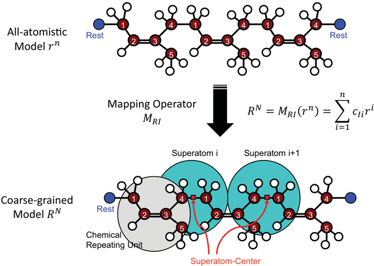
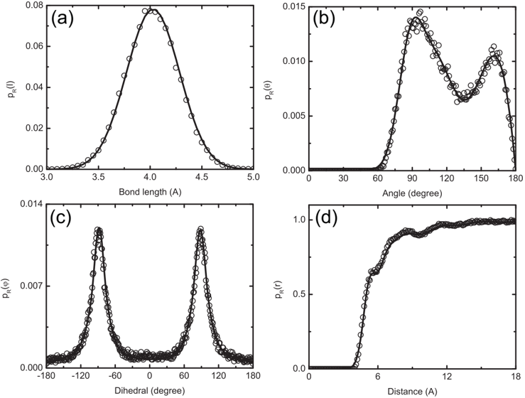
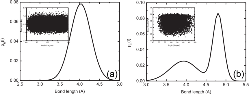
“One is the center of the PI monomer, and the other is the center of the carbon-carbon bond connecting two monomers together.The distribution functions, p R (l), for both of these definitions have been obtained (Figure 10).In the first case, p R (l) is characterized well by a single Gaussian”
§ Challenges in Multiscale Modeling of Polymer Dynamics > 4.1.1. Definition of Super Atom
“if the super-atomic center is defined as the center of mass of the cis-PI monomer (i.e., the carbon-carbon double bond), the p R (l) will have two peaks”
Rated minor: it would not touch a result — a value no result rests on, a p-value that stays on the same side of the significance level, or a conflict that is clerical, resolved elsewhere in the paper, or outside its own findings.
In the paper
§ Challenges in Multiscale Modeling of Polymer Dynamics > 3.3. Slip-Link Model
“the G(t) given by the Doi-Edwards model decays very quickly, compared with the slip-link model, since the Doi-Edwards model only considers reptation, whereas the slip-link model contains other relaxation mechanisms, i.e., the chain fluctuation and constraint release.”
§ Challenges in Multiscale Modeling of Polymer Dynamics > 1. Introduction
“Thus, CR is a cooperative phenomenon between different chains, while CLF can be considered as a single-chain phenomenon, but both hasten the relaxation process.”
Rated minor: it would not touch a result — a value no result rests on, a p-value that stays on the same side of the significance level, or a conflict that is clerical, resolved elsewhere in the paper, or outside its own findings.
In the paper
§ Challenges in Multiscale Modeling of Polymer Dynamics > 5.3. Concurrent Modeling of Polymer Melts under Shear Flow
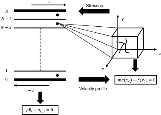
“Equations ( 35) and ( 36) are for the fine scale (MD), scale bridging (modified virial stress) and the coarse scale (continuum), respectively.”
§ Challenges in Multiscale Modeling of Polymer Dynamics > 5.3. Concurrent Modeling of Polymer Melts under Shear Flow
“mq (x ζ ) -f (x ζ ) = 0 for x ζ ∈ Θ ζ (35 ) ρü(x ζ ) -∇ • σ(x ζ ) = 0 for x ζ ∈ Ω (36 ) σ(x ζ ) = 1 2Θ ζ A B =A r AB ζ (x ζ ) ⊗ f AB ζ (x ζ )(37)”
Citations
Cites
Items 201–400 of 412
Screening of hydrodynamic interactions in semidilute polymer solutions: A computer simulation study
Ahlrichs, P., Everaers, R., & Dünweg, B. (2001) · Physical Review E · doi:10.1103/physreve.64.040501 · Cited by 107 · cited 1×
“Compared with polymer melts, particular attention must be paid to the solvent-mediation effect between polymeric beads, also called hydrodynamic interaction [361].”
BackgroundDynamics of n-alkanes: Comparison to Rouse ModelPreprint
Mondello, M., Grest, G. S., Webb, E. B., III, Peczak, P., & Milner, S. T. (1998) · Cited by 105
From mesoscale back to atomistic models: A fast reverse-mapping procedure for vinyl polymer chains
Santangelo, G., Di Matteo, A., Müller-Plathe, F., & Milano, G. (2007) · The Journal of Physical Chemistry B · doi:10.1021/jp066212l · Cited by 104 · cited 1×
“As the equilibration of a coarse-grained polymer is much faster and easier than the all-atomistic one, the back-mapping procedure can be used to quickly generate equilibrated all-atomistic models of highly entangled polymers, including polycarbonates [177,235,341], polystyrene [198,201] and polyamide [197,342].”
MethodRheological Properties of 1,4-Polyisoprene over a Large Molecular Weight Range
Abdel-Goad, M., Pyckhout-Hintzen, W., Kahle, S., Allgaier, J., Richter, D., & Fetters, L. J. (2004) · Macromolecules · doi:10.1021/ma030557+ · Cited by 103 · cited 1×
“The dots are experimental results taken from [332].”
BackgroundMultiscale simulation in polymer science
Kremer, K., & Müller‐Plathe, F. (2002) · Molecular Simulation · doi:10.1080/0892702021000002458 · Cited by 102 · cited 1×
“There exist some excellent and recent reviews on the coarse-graining of entangled polymers, focusing on static properties [35–37], dynamic properties [38–41] and the comparison between different”
BackgroundHu, Y., Wang, S. Q., & Jamieson, A. M. (1993) · Journal of Rheology · doi:10.1122/1.550458 · Cited by 101 · cited 1×
“These behaviors are experimentally observed [314,315] and have also been captured by different constitutive models [316,317]; however, these models tend to exhibit the inconvenient feature that they describe some types of flow very well, while failing for others [19].”
BackgroundMorphology Control of Hairy Nanopores
Peleg, O., Tagliazucchi, M., Kröger, M., et al. (2011) · ACS Nano · doi:10.1021/nn200702u · Cited by 100 · cited 1×
“nanopores [58]; and the effect of charge, hydrophobicity and sequence of nucleoporins on the translocation of model particles through the nuclear pore complex [59]; to mention a few.”
BackgroundSelf-citationA coupled quantum/continuum mechanics study of graphene fracture
Xu, M., Tabarraei, A., Paci, J. T., et al. (2012) · International Journal of Fracture · doi:10.1007/s10704-011-9675-x · Cited by 100 · cited 1×
“There is a tremendous amount of concurrent multiscale modeling methods developed in the recent ten years with rigorous mathematical foundations, but mostly for metals [344,346–350] and carbon nanomaterials [345,351–354].”
BackgroundCoding coarse grained polymer model for LAMMPS and its application to polymer crystallization
Luo, C., & Sommer, J. (2009) · Computer Physics Communications · doi:10.1016/j.cpc.2009.01.028 · Cited by 99 · cited 1×
“Luo and Sommer [208] developed a tabulated angle potential function with cubic spline interpolation to smooth both potential and force in simulations.”
BackgroundHarmandaris, V. A., Doxastakis, M., Mavrantzas, V. G., & Theodorou, D. N. (2002) · The Journal of Chemical Physics · doi:10.1063/1.1416872 · Cited by 98 · cited 2×
“The united-atom method involves ignoring hydrogen atoms and is reviewed in [2,3].”
BackgroundMethodEveraers, R. (2012) · Physical Review E · doi:10.1103/physreve.86.022801 · Cited by 96 · cited 3×
“Recently, Everaers [286] compared the entanglement length, N e , given by the PPA, tube models and slip-link models, and proposed a simple relationship between topological and rheological entanglement length.”
InfluentialStochastic Eulerian Lagrangian methods for fluid–structure interactions with thermal fluctuations
Atzberger, P. J. (2011) · Journal of Computational Physics · doi:10.1016/j.jcp.2010.12.028 · Cited by 94
Quantitative predictions of linear viscoelastic rheological properties of entangled polymers
Pattamaprom, C., Larson, R. G., & Dyke, T. J. V. (2000) · Rheologica Acta · doi:10.1007/s003970000104 · Cited by 94 · cited 2×
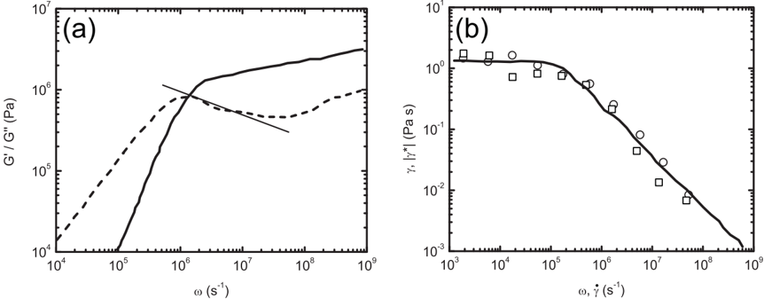
“In Figure 19a, the Ψ (t) is compared with the double reptation model [295,296] and dual constraint model [297,298].”
BackgroundMethodDepa, P. K., & Maranas, J. K. (2005) · The Journal of Chemical Physics · doi:10.1063/1.1997150 · Cited by 94 · cited 1×
“Although such a dynamic rescaling method does not have rigorous theoretical foundations, it has been used successfully for low degrees of coarse graining [92,183,184,197,200,201,221–227].”
MethodModeling polyethylene with the bond fluctuation model
Tries, V., Paul, W., Baschnagel, J., & Binder, K. (1997) · The Journal of Chemical Physics · doi:10.1063/1.473162 · Cited by 94 · cited 1×
“Subsequent works focused on the mapping of BFM results to real polymers, such as bisphenol polycarbonates and polyethylene (PE) [99–102].”
BackgroundUchida, N., Grest, G. S., & Everaers, R. (2008) · The Journal of Chemical Physics · doi:10.1063/1.2825597 · Cited by 93 · cited 4×
“The obtained results agree with experimental observations of the normalized plateau moduli of both loosely and tightly entangled polymers over 13 decades in frequency space, from 10−6 to 10(7) s−1 [120].”
MethodResultInfluentialGoujon, F., Malfreyt, P., & Tildesley, D. J. (2008) · The Journal of Chemical Physics · doi:10.1063/1.2954022 · Cited by 92 · cited 1×
“[249], who developed a repulsive potential between segments [250] in DPD simulation to avoid bond crossing.”
BackgroundAdvanced Computer Simulation Approaches for Soft Matter Sciences II
Holm, C., & Kremer, K. (2005) · Springer eBooks · doi:10.1007/b136792 · Cited by 91
Milano, G., Goudeau, S., & Müller‐Plathe, F. (2005) · Journal of Polymer Science Part B: Polymer Physics · doi:10.1002/polb.20380 · Cited by 90 · cited 3×
“[196] developed and discussed analytical forms for these complex distribution functions.”
BackgroundStructure-property correlation of polymers, a Monte Carlo approach
Paul, W., Binder, K., Kremer, K., & Heermann, D. W. (1991) · Macromolecules · doi:10.1021/ma00023a041 · Cited by 90 · cited 1×
“Subsequent works focused on the mapping of BFM results to real polymers, such as bisphenol polycarbonates and polyethylene (PE) [99–102].”
BackgroundPredicting polymer dynamics at multiple length and time scales
Harmandaris, V. A., & Kremer, K. (2009) · Soft Matter · doi:10.1039/b905361a · Cited by 90 · cited 9×
“Conversely, the well-equilibrated coarse-grained models can be mapped back onto an atomistic model, as reviewed by Müller-Plathe [38] and Peter and Kremer [340].”
MethodInfluentialCoarse graining of short polythylene chains for studying polymer crystallization
Vettorel, T., & Meyer, H. (2006) · Journal of Chemical Theory and Computation · doi:10.1021/ct0503264 · Cited by 90 · cited 1×
“For homopolymer melts, for example, polyethylene [237], polybutadiene [226,238] and other polymers, the coarse-grained potentials show a remarkable transferability over a large range of temperatures.”
BackgroundDiffusion of linear polystyrene molecules in matrixes of different molecular weights
Antonietti, M., Coutandin, J., & Sillescu, H. (1986) · Macromolecules · doi:10.1021/ma00157a051 · Cited by 90 · cited 1×
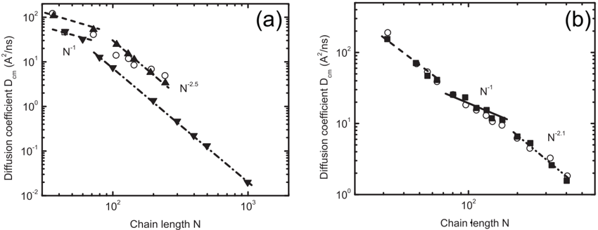
“In (a), the scaled diffusion coefficient, D(N)/DR(N), is plotted against the scaled chain length, N/Ne,p, for polystyrene (closed circles Ne,p = 140 and T = 485 K [111]), polyethylene (closed squares Ne,p = 31 and T = 448 K [112]), hydrogenated polybutadiene (closed triangles Ne,p = 18 and T = 448 K [113]), FENE (open…”
BackgroundSystematic coarse-graining of atomistic models for simulation of polymeric systems
Sun, Q., & Faller, R. (2005) · Computers & Chemical Engineering · doi:10.1016/j.compchemeng.2005.05.026 · Cited by 88 · cited 2×
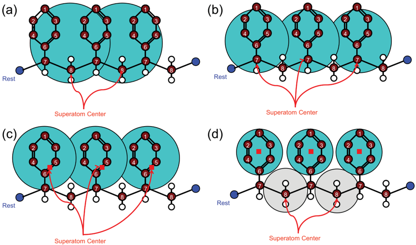
“Sun and Faller systematically developed a coarse-grained model for isotactic PS melts from the unentangled to the entangled regime using the super atom definition shown in Figure 11b [185,200].”
BackgroundMethodChen, C., Depa, P. K., Sakai, V. G., Maranas, J. K., Lynn, J. W., Peral, I., & Copley, J. R. D. (2006) · The Journal of Chemical Physics · doi:10.1063/1.2204035 · Cited by 87 · cited 1×
“Although such a dynamic rescaling method does not have rigorous theoretical foundations, it has been used successfully for low degrees of coarse graining [92,183,184,197,200,201,221–227].”
MethodConditional reversible work method for molecular coarse graining applications
Brini, E., Marcon, V., & van der Vegt, N. F. A. (2011) · Physical Chemistry Chemical Physics · doi:10.1039/c0cp02888f · Cited by 87 · cited 1×
“There are three methods belonging to the derived coarse-graining methods: pair potential of mean force [160], effective force coarse-graining [162] and conditional reversible work [163].”
MethodTwo-scale mechanism-based theory of nonlinear viscoelasticity
Tang, S., Steven Greene, M., & Liu, W. K. (2012) · Journal of the Mechanics and Physics of Solids · doi:10.1016/j.jmps.2011.11.003 · Cited by 87 · cited 10×
“According to the tube model [5,6], assumed to describe the motion of these free chains, the viscous Cauchy stress can be formulated as [32]:”
BackgroundMethodInfluentialSelf-citationCoarse-grained modeling of polystyrene in various environments by iterative Boltzmann inversion
Bayramoglu, B., & Faller, R. (2012) · Macromolecules · doi:10.1021/ma301280b · Cited by 86 · cited 5×
“Sun and Faller systematically developed a coarse-grained model for isotactic PS melts from the unentangled to the entangled regime using the super atom definition shown in Figure 11b [185,200].”
BackgroundMethodInfluentialJayaraman, A., & Schweizer, K. S. (2008) · Macromolecules · doi:10.1021/ma801722m · Cited by 86 · cited 1×
“Such important understanding will enhance our capability to process and design PNCs with targeted mechanical and physical properties, as discussed extensively in [328,329,377,379–382,386–391].”
BackgroundCrossover from unentangled to entangled dynamics in a systematically coarse-grained polystyrene melt
Sun, Q., & Faller, R. (2006) · Macromolecules · doi:10.1021/ma0514774 · Cited by 85 · cited 2×
“Sun and Faller systematically developed a coarse-grained model for isotactic PS melts from the unentangled to the entangled regime using the super atom definition shown in Figure 11b [185,200].”
BackgroundMethodScale-Hopping in Computer Simulations of Polymers
Müller-Plathe, F. (2002) · Soft Materials · doi:10.1081/smts-120016739 · Cited by 85 · cited 1×
“There exist some excellent and recent reviews on the coarse-graining of entangled polymers, focusing on static properties [35–37], dynamic properties [38–41] and the comparison between different”
BackgroundHua, C. C., Schieber, J. D., & Venerus, D. C. (1998) · The Journal of Chemical Physics · doi:10.1063/1.477671 · Cited by 85 · cited 6×
“To further extend the spatial and temporal scales of these generic simulation methods, Hua and Schieber [33,80,81] performed the pioneering works in developing the slip-link model, based on the concept of the tube model, as illustrated in Figure 5a.”
BackgroundMethodInfluentialViscoelasticity and Molecular Rheology
Likhtman, A. E. (2012) · Elsevier eBooks · doi:10.1016/b978-0-444-53349-4.00008-x · Cited by 83
Kröger, M., & Makhloufi, R. (1996) · Physical Review E · doi:10.1103/physreve.53.2531 · Cited by 83 · cited 1×
“and recombination in worm-like micelles and equilibrium polymers [131–134], surface tension [135], dielectric relaxation [136], polymer welding [137,138], strain hardening [121,122] and other properties.”
BackgroundSelf-citationMurtola, T. J., Falck, E., Karttunen, M., & Vattulainen, I. (2007) · The Journal of Chemical Physics · doi:10.1063/1.2646614 · Cited by 82 · cited 1×
“[213] adopted thermodynamic constraints in the IMC method to improve the convergence.”
MethodRod-like colloids and polymers in shear flow: A multi-particle-collision dynamics study
Winkler, R. G., Mussawisade, K., Ripoll, M., & Gompper, G. (2004) · Journal of Physics: Condensed Matter · doi:10.1088/0953-8984/16/38/012 · Cited by 81 · cited 1×
“In order to avoid modeling the solvent explicitly, some techniques have been developed recently, such as dissipative particle dynamics [362], stochastic rotation dynamics [363,364] and the lattice Boltzmann method [365,366].”
MethodRecent progress on polymer dynamics by neutron scattering: From simple polymers to complex materials
Colmenero, J., & Arbe, A. (2012) · Journal of Polymer Science Part B Polymer Physics · doi:10.1002/polb.23178 · Cited by 81 · cited 1×
“For this reason, many computational and experimental works have been performed in recent years to understand the polymer dynamics at the interface and in the interphase [127,128,328,329,370–382].”
BackgroundShear Banding in Molecular Dynamics of Polymer Melts
Cao, J., & Likhtman, A. E. (2012) · Physical Review Letters · doi:10.1103/physrevlett.108.028302 · Cited by 80 · cited 1×
“Although recent MD simulation of FENE chains reproduces shear banding [358], it is a simple, brute-force approach.”
MethodZhou, Q., & Larson, R. G. (2005) · Macromolecules · doi:10.1021/ma050347s · Cited by 79 · cited 1×
“Within the original PPA method, the PP was defined as the path with minimum total energy, not as the shortest path between two ends of the chain, and PPA results are known to weakly depend on implementation details, such as a temperature ramp and bead size [276,287].”
MethodTzoumanekas, C., & Theodorou, D. N. (2006) · Current Opinion in Solid State and Materials Science · doi:10.1016/j.cossms.2006.11.003 · Cited by 78 · cited 1×
“Since the rheological properties of entangled polymer melts are dominated by entanglements, many computational works have been undertaken to extract the underlying primitive path (PP) and entanglement characteristics predicted by the tube model directly from the atomistic simulations [76,79,97,119,178,198,223,242,275–…”
BackgroundStudying the origin of strain hardening: Basic difference between extension and shear
Liu, G., Sun, H., Rangou, S., Ntetsikas, K., Avgeropoulos, A., & Wang, S.-Q. (2013) · Journal of Rheology · doi:10.1122/1.4763568 · Cited by 77 · cited 1×
“, shear thinning and normal stress differences in shear flow [315,355], strain hardening in elongation [356] and shear banding [357].”
BackgroundMapping of Explicit Atom onto United Atom Potentials
McCoy, J. D., & Curro, J. G. (1998) · Macromolecules · doi:10.1021/ma981060g · Cited by 77 · cited 1×
“In most studies, the super atom is defined to be a spherical particle [37,177,184,189–191], but there are also some studies attempting to do generalizations for anisotropic potentials [192,193].”
BackgroundEslami, H., & Müller-Plathe, F. (2013) · The Journal of Physical Chemistry C · doi:10.1021/jp400142h · Cited by 76 · cited 1×
“To address this issue, Bayramoglu and Faller [240] and Müller-Plathe and his co-workers [239,385] adopted a systematic coarse-graining method, the IBI method, to study confined polystyrene and Polyamide-6,6, respectively.”
MethodPeter, S., Napolitano, S., Meyer, H., Wübbenhorst, M., & Baschnagel, J. (2008) · Macromolecules · doi:10.1021/ma800694v · Cited by 76 · cited 1×
“and recombination in worm-like micelles and equilibrium polymers [131–134], surface tension [135], dielectric relaxation [136], polymer welding [137,138], strain hardening [121,122] and other properties.”
BackgroundGlass Transition Behavior of Polymer Films of Nanoscopic Dimensions
Baljon, A. R. C., van Weert, M. H. M., DeGraaff, R. B., & Khare, R. (2005) · Macromolecules · doi:10.1021/ma048819a · Cited by 76 · cited 2×
“With the attractive well, the FENE model has been applied to study the glass transition temperature [127–130], scission”
BackgroundMethodStep shear of entangled linear polymer melts: New experimental evidence for elastic yielding
Boukany, P. E., Wang, S.-Q., & Wang, X. (2009) · Macromolecules · doi:10.1021/ma9004346 · Cited by 76 · cited 1×
“, shear thinning and normal stress differences in shear flow [315,355], strain hardening in elongation [356] and shear banding [357].”
BackgroundTopological entanglement length in polymer melts and nanocomposites by a DPD polymer model
Karatrantos, A., Clarke, N., Composto, R. J., & Winey, K. I. (2013) · Soft Matter · doi:10.1039/c3sm27651a · Cited by 76 · cited 1×
“DPD polymers is found to be consistent with the classical MD simulations [247,248].”
ResultStructure and Rheology of Molten Polymers
Dealy, J. M., & Larson, R. G. (2006) · doi:10.3139/9783446412811.fm · Cited by 75
A constitutive equation for graphene based on density functional theory
Xu, M., Paci, J. T., Oswald, J., et al. (2012) · International Journal of Solids and Structures · doi:10.1016/j.ijsolstr.2012.05.019 · Cited by 75 · cited 1×
“There is a tremendous amount of concurrent multiscale modeling methods developed in the recent ten years with rigorous mathematical foundations, but mostly for metals [344,346–350] and carbon nanomaterials [345,351–354].”
BackgroundStructure, dimensions, and entanglement statistics of long linear polyethylene chains
Foteinopoulou, K., Karayiannis, N. C., Laso, M., & Kröger, M. (2009) · The Journal of Physical Chemistry B · doi:10.1021/jp808287s · Cited by 74 · cited 1×
“Through static PP analysis using Z1 code, all these parameters, except α, can be directly obtained [92,178,242,330].”
MethodSelf-citationYaoita, T., Isaki, T., Masubuchi, Y., Watanabe, H., Ianniruberto, G., & Marrucci, G. (2011) · Macromolecules · doi:10.1021/ma202166y · Cited by 74 · cited 1×
“also extended to study star and branched polymers [150], nonlinear rheology [151–153], phase separation in polymer blends [154,155], block copolymers [156] and the dynamics of confined polymers [157].”
BackgroundPeter, S., Meyer, H., Baschnagel, J., & Seemann, R. (2007) · Journal of Physics Condensed Matter · doi:10.1088/0953-8984/19/20/205119 · Cited by 71 · cited 1×
“With the attractive well, the FENE model has been applied to study the glass transition temperature [127–130], scission”
MethodReal Space Structure and Scattering Patterns of Model Polymer Nanocomposites
Hooper, J. B., & Schweizer, K. S. (2007) · Macromolecules · doi:10.1021/ma071147e · Cited by 71 · cited 1×
“Such important understanding will enhance our capability to process and design PNCs with targeted mechanical and physical properties, as discussed extensively in [328,329,377,379–382,386–391].”
BackgroundSystematic Coarse-Graining of a Polymer Blend: Polyisoprene and Polystyrene
Sun, Q., & Faller, R. (2006) · Journal of Chemical Theory and Computation · doi:10.1021/ct600065v · Cited by 71 · cited 1×
“Similar behavior is also found in cis-1-4 PI and trans-PI polymers by Faller and his co-workers [37,68,182–186].”
ResultProperties of Poly(isoprene): Model Building in the Melt and in Solution
Faller, R., & Reith, D. (2003) · Macromolecules · doi:10.1021/ma025877s · Cited by 70 · cited 3×
“In most studies, the super atom is defined to be a spherical particle [37,177,184,189–191], but there are also some studies attempting to do generalizations for anisotropic potentials [192,193].”
BackgroundMethodResultPrimitive chain network study on uncrosslinked and crosslinked cis-polyisoprene polymers
Li, Y., Kröger, M., & Liu, W. K. (2011) · Polymer · doi:10.1016/j.polymer.2011.10.044 · Cited by 70 · cited 2×
“Through static PP analysis using Z1 code, all these parameters, except α, can be directly obtained [92,178,242,330].”
MethodSelf-citationUchida, N., Grest, G. S., & Everaers, R. (2008) · Max Planck Institute for Plasma Physics · Cited by 70
Theoretical models for bridging timescales in polymer dynamics
Guenza, M. G. (2008) · Journal of Physics: Condensed Matter · doi:10.1088/0953-8984/20/03/033101 · Cited by 70 · cited 1×
“(ii) Analytical super coarse-graining method [87,88] Section 4.”
MethodPolymer + Solvent Systems: Phase Diagrams, Interface Free Energies, and Nucleation
Binder, K., Müller, M., Virnau, P., & MacDowell, L. G. (2005) · Advances in polymer science · doi:10.1007/b99426 · Cited by 69
Fluctuating soft-sphere approach to coarse-graining of polymer models
Vettorel, T., Besold, G., & Kremer, K. (2010) · Soft Matter · doi:10.1039/b921159d · Cited by 69 · cited 1×
“More recently, the method has been extended to chains of Gaussian blobs by Pierleoni and his co-workers [253,254] and Kremer and his co-workers [255,256], allowing for much more efficient implementations.”
MethodHarmandaris, V. A., Floudas, G., & Kremer, K. (2011) · Macromolecules · doi:10.1021/ma102179b · Cited by 69 · cited 9×
“Conversely, the well-equilibrated coarse-grained models can be mapped back onto an atomistic model, as reviewed by Müller-Plathe [38] and Peter and Kremer [340].”
BackgroundMethodInfluentialAkutagawa, K., Yamaguchi, K., Yamamoto, A., Heguri, H., Jinnai, H., & Shinbori, Y. (2008) · Rubber Chemistry and Technology · doi:10.5254/1.3548203 · Cited by 68 · cited 3×
“This agrees with the three- to 13-fold strain localization observed in the experiments [398,399].”
BackgroundResultMasubuchi, Y., Ianniruberto, G., Greco, F., & Marrucci, G. (2004) · Modelling and Simulation in Materials Science and Engineering · doi:10.1088/0965-0393/12/3/s03 · Cited by 68 · cited 1×
“Later on, the PCN model was extended to study the relationship between entanglement length and plateau modulus [145–149].”
MethodAnalytical soft-core potentials for macromolecular fluids and mixtures
Yatsenko, G., Sambriski, E. J., Nemirovskaya, M. A., & Guenza, M. (2004) · Physical Review Letters · doi:10.1103/physrevlett.93.257803 · Cited by 68 · cited 1×
“For N > 30, the approximation of hcc given above is exact [73,274].”
BackgroundHarmandaris, V., Adhikari, N. P., van der Vegt, N. F. A., Kremer, K., Mann, B. A., Voelkel, R., Weiss, H., & Liew, C. (2007) · Macromolecules · doi:10.1021/ma070201o · Cited by 68 · cited 1×
“However, there are several studies demonstrating that the effective potential functions of the coarse-grained model have a limited range of transferability into a subset of thermodynamics states [69,188,201,231–236].”
BackgroundDeviations from dynamic dilution in the terminal relaxation of star polymers
Shanbhag, S., Larson, R. G., Takimoto, J., & Doi, M. (2001) · Physical Review Letters · doi:10.1103/physrevlett.87.195502 · Cited by 68 · cited 1×
“[139] developed a dual slip-link model with chain-end fluctuations for entangled star polymers, which explained the observed deviations from the “dynamic dilution” equation in the dielectric and stress relaxation data.”
BackgroundMasubuchi, Y., Ianniruberto, G., Greco, F., & Marrucci, G. (2007) · Journal of Non-Newtonian Fluid Mechanics · doi:10.1016/j.jnnfm.2007.02.014 · Cited by 67 · cited 1×
“Later on, the PCN model was extended to study the relationship between entanglement length and plateau modulus [145–149].”
MethodFish, J., Chen, W., & Li, R. (2006) · Computer Methods in Applied Mechanics and Engineering · doi:10.1016/j.cma.2006.08.001 · Cited by 67 · cited 1×
“a Lagrangian framework by following the generalized mathematical homogenization theory [321–323] for different scales:”
MethodPadding, J. T., & Briels, W. J. (2001) · The Journal of Chemical Physics · doi:10.1063/1.1368135 · Cited by 67 · cited 1×
“By following the same principle of the IBI method, the potential functions for the blob model were systematically derived from the all-atomistic simulation [243].”
MethodKirkwood–Buff Coarse-Grained Force Fields for Aqueous Solutions
Ganguly, P., Mukherji, D., Junghans, C., & van der Vegt, N. F. A. (2012) · Journal of Chemical Theory and Computation · doi:10.1021/ct3000958 · Cited by 67 · cited 1×
“The structure-based methods include the iterative Boltzmann inversion (IBI) method [82,83], the Kirkwood-Buff IBI method [164], the inverse Monte Carlo (IMC) method [165], the relative entropy method [166] and the generalized Yvon–Born–Green theory [167].”
MethodA single particle model to simulate the dynamics of entangled polymer melts
Kindt, P., & Briels, W. J. (2007) · The Journal of Chemical Physics · doi:10.1063/1.2780151 · Cited by 66 · cited 15×
“As shown in Figure 14, Padding and Briels applied the blob model to study PE polymer melts with chain lengths ranging between 80 and 1000 (blobs from four to 50) [85].”
BackgroundMethodInfluentialFirst-principle approach to rescale the dynamics of simulated coarse-grained macromolecular liquids
Lyubimov, I., & Guenza, M. G. (2011) · Physical Review E · doi:10.1103/physreve.84.031801 · Cited by 66 · cited 10×
“Thus, in the coarse-graining process, the internal friction coefficient between monomers is typically also changed, leading to incorrect dynamic behavior of the coarse-grained system [37,217,218].”
BackgroundMethodInfluentialDoxastakis, M., Mavrantzas, V. G., & Theodorou, D. N. (2001) · The Journal of Chemical Physics · doi:10.1063/1.1416490 · Cited by 66
Halperin, A., & Kröger, M. (2012) · Biomaterials · doi:10.1016/j.biomaterials.2012.03.060 · Cited by 64 · cited 1×
“number of important applications were newly added in the recent past, including block copolymers and nanocomposites [53]; screening effects in polyelectrolyte brushes [54]; mixed polymer brushes [55]; harvesting cells cultured on thermoresponsive polymer brushes [56,57]; morphology control of hairy”
BackgroundSelf-citationComparison of Constitutive Equations For Melts
Larson, R. G. (1988) · Constitutive Equations for Polymer Melts and Solutions · doi:10.1016/b978-0-409-90119-1.50012-9 · Cited by 64
Anogiannakis, S. D., Tzoumanekas, C., & Theodorou, D. N. (2012) · Macromolecules · doi:10.1021/ma300912z · Cited by 63 · cited 1×
“Since the rheological properties of entangled polymer melts are dominated by entanglements, many computational works have been undertaken to extract the underlying primitive path (PP) and entanglement characteristics predicted by the tube model directly from the atomistic simulations [76,79,97,119,178,198,223,242,275–…”
BackgroundMolecular dynamics of model liquid crystals composed of semiflexible molecules
Affouard, F., Kröger, M., & Hess, S. (1996) · Physical review. E, Statistical physics, plasmas, fluids, and related interdisciplinary topics · doi:10.1103/physreve.54.5178 · Cited by 63 · cited 1×
“To overcome these issues, a backbone bending potential was incorporated into the FENE model as Vbend = kbend[1 − cos(θ − θ0)], where θ0 = 180◦ is the equilibrium angle [116].”
MethodSelf-citationMolecular dynamics study of entangled hard-chain fluids
Smith, S. W., Hall, C. K., & Freeman, B. D. (1996) · The Journal of Chemical Physics · doi:10.1063/1.471802 · Cited by 62 · cited 1×
“45 [114]).”
Coarse-grained computer simulation of nanoconfined polyamide-6, 6
Eslami, H., Karimi-Varzaneh, H. A., & Müller-Plathe, F. (2011) · Macromolecules · doi:10.1021/ma102320v · Cited by 61 · cited 2×
“To address this issue, Bayramoglu and Faller [240] and Müller-Plathe and his co-workers [239,385] adopted a systematic coarse-graining method, the IBI method, to study confined polystyrene and Polyamide-6,6, respectively.”
BackgroundMethodYieldlike constitutive transition in shear flow of entangled polymeric fluids
Tapadia, P., & Wang, S.-Q. (2003) · Physical Review Letters · doi:10.1103/physrevlett.91.198301 · Cited by 60 · cited 2×
“, shear thinning and normal stress differences in shear flow [315,355], strain hardening in elongation [356] and shear banding [357].”
BackgroundThermodynamic consistency in variable-level coarse graining of polymeric liquids
Clark, A. J., McCarty, J., Lyubimov, I. Y., & Guenza, M. G. (2012) · Physical Review Letters · doi:10.1103/physrevlett.109.168301 · Cited by 60 · cited 1×
“The structure and thermodynamic consistency between the all-atomistic model and its corresponding super coarse-grained model has also been studied and verified [270,271].”
BackgroundToth, R., Voorn, D. J., Handgraaf, J., et al. (2009) · Macromolecules · doi:10.1021/ma901584w · Cited by 60
Transient forces in flowing soft matter
Briels, W. J. (2009) · Soft Matter · doi:10.1039/b911310j · Cited by 59 · cited 2×
“be quadratic in the deviations of n0, originating from a penalty free energy equation [259].”
BackgroundTopological Structure and Nonaffine Swelling of Bimodal Polymer Networks
Sommer, J., & Lay, S. (2002) · Macromolecules · doi:10.1021/ma0205515 · Cited by 59 · cited 1×
“Such differences imply the existence of non-affine deformation [26,337–339].”
BackgroundOn the frequency and amplitude dependence of the Payne effect: Theory and experiments
Lion, A., Kardelky, C., & Haupt, P. (2003) · Rubber Chemistry and Technology · doi:10.5254/1.3547759 · Cited by 58 · cited 1×
“Several constitutive models [333,394] have been developed to characterize this important feature, incorporating the concept of occlusion to account for the breakage of weak physical bonds.”
BackgroundCoarse-Grained Modeling for Macromolecular Chemistry
Karimi‐Varzaneh, H. A., & Müller‐Plathe, F. (2011) · Topics in current chemistry · doi:10.1007/128_2010_122 · Cited by 58 · cited 1×
“Although such a dynamic rescaling method does not have rigorous theoretical foundations, it has been used successfully for low degrees of coarse graining [92,183,184,197,200,201,221–227].”
MethodReptation of a Polymer Chain in the Presence of Fixed Obstacles
de Gennes, P. G. (2009) · Series on directions in condensed matter physics · doi:10.1142/9789814280648_0004 · Cited by 57
Chen, C., Depa, P. K., Maranas, J. K., & Sakai, V. G. (2008) · The Journal of Chemical Physics · doi:10.1063/1.2833545 · Cited by 57 · cited 1×
“Although such a dynamic rescaling method does not have rigorous theoretical foundations, it has been used successfully for low degrees of coarse graining [92,183,184,197,200,201,221–227].”
MethodThe state of the art in the rheology of polymers: Achievements and challenges
Malkin, A. Y. (2009) · Polymer Science Series A · doi:10.1134/s0965545x09010076 · Cited by 57 · cited 1×
“Polymer flow in dilute solution is also an interesting and challenging problem [360].”
BackgroundIlg, P., Kröger, M., & Hess, S. (2005) · Physical Review E · doi:10.1103/physreve.71.031205 · Cited by 56
Self-citationFailure-mode transition in transient polymer networks with particle-based simulations
Sprakel, J., Spruijt, E., van der Gucht, J., Padding, J. T., & Briels, W. J. (2009) · Soft Matter · doi:10.1039/b910425a · Cited by 56 · cited 1×
“The transient force model has been demonstrated to correctly reproduce the large temporal linear and nonlinear rheological properties of linear polymer melts [86,261,262], telechelic [263] and star polymers [264] and polymeric adhesives [265,266].”
MethodOnset of Entanglements Revisited. Topological Analysis
Tzoumanekas, C., Lahmar, F., Rousseau, B., & Theodorou, D. N. (2009) · Macromolecules · doi:10.1021/ma901131c · Cited by 55
Theoretically informed entangled polymer simulations: linear and non-linear rheology of melts
Ramírez-Hernández, A., Müller, M., & Pablo, J. (2013) · Soft Matter · doi:10.1039/c2sm26674a · Cited by 55 · cited 1×
“presented a more general formalism based on the slip-link model to quantitatively capture the linear rheology of pure homopolymers and their blends, as well as the nonlinear rheology of highly entangled polymers and the dynamics of diblock copolymers [159].”
BackgroundEntanglement Relaxation Time in Polyethylene: Simulation versus Experimental Data
Ramos, J., Vega, J. F., Theodorou, D. N., & Martinez-Salazar, J. (2008) · Macromolecules · doi:10.1021/ma702445e · Cited by 55 · cited 1×
“In (a), the dots are experimental results [334].”
BackgroundStrain inhomogeneity and discontinuous crack growth in a particulate composite
Gonzalez, J., & Knauss, W. G. (1998) · Journal of the Mechanics and Physics of Solids · doi:10.1016/s0022-5096(98)00037-4 · Cited by 55 · cited 1×
“This agrees with the three- to 13-fold strain localization observed in the experiments [398,399].”
ResultPaul, W., & Pistoor, N. (1994) · Macromolecules · doi:10.1021/ma00083a027 · Cited by 54 · cited 1×
“Subsequent works focused on the mapping of BFM results to real polymers, such as bisphenol polycarbonates and polyethylene (PE) [99–102].”
BackgroundLocal Structure and Dynamics of trans-Polyisoprene Oligomers
Faller, R., Müller‐Plathe, F., Doxastakis, M., & Theodorou, D. N. (2001) · Macromolecules · doi:10.1021/ma0016782 · Cited by 53 · cited 1×
“Similar behavior is also found in cis-1-4 PI and trans-PI polymers by Faller and his co-workers [37,68,182–186].”
ResultWhy is understanding glassy polymer mechanics so difficult?
Hoy, R. S. (2011) · Journal of Polymer Science Part B: Polymer Physics · doi:10.1002/polb.22276 · Cited by 53 · cited 2×
“Therefore, including the bending potential into the FENE model is a very common extension [16,121–123].”
BackgroundResultEntanglements and dynamics of polymer melts near a SWCNT
Karatrantos, A., Composto, R. J., Winey, K. I., Kröger, M., & Clarke, N. (2012) · Macromolecules · doi:10.1021/ma3007637 · Cited by 53 · cited 1×
“DPD polymers is found to be consistent with the classical MD simulations [247,248].”
ResultSelf-citationSystematic time-scale-bridging molecular dynamics applied to flowing polymer melts
Ilg, P., Öttinger, H. C., & Kröger, M. (2009) · Physical Review E · doi:10.1103/physreve.79.011802 · Cited by 52 · cited 5×
“(iii) Molecularly-derived constitutive equation [90] Section 5.”
BackgroundMethodInfluentialSelf-citationNusser, K., Schneider, G. J., & Richter, D. (2011) · Soft Matter · doi:10.1039/c1sm05555k · Cited by 52 · cited 7×
“Is there a glassy polymer layer near the surface of NPs in PNCs?”
BackgroundResultInfluentialThermomechanical properties of the WCA–Lennard-Jones model system in its fluid and solid states
Hess, S., Kröger, M., & Voigt, H. (1998) · Physica A: Statistical Mechanics and its Applications · doi:10.1016/s0378-4371(97)00612-2 · Cited by 52 · cited 1×
“Additionally, several monomers are coarse-grained into one bead, which greatly reduces the degrees of freedom, and the Einstein frequency determining the MD time step is basically set by the WCA potential, whose thermo-mechanical properties are well known [104].”
BackgroundSelf-citationComparison among Slip-Link Simulations of Bidisperse Linear Polymer Melts
Masubuchi, Y., Watanabe, H., Ianniruberto, G., Greco, F., & Marrucci, G. (2008) · Macromolecules · doi:10.1021/ma800954q · Cited by 52 · cited 1×
“also extended to study star and branched polymers [150], nonlinear rheology [151–153], phase separation in polymer blends [154,155], block copolymers [156] and the dynamics of confined polymers [157].”
BackgroundAnalytical rescaling of polymer dynamics from mesoscale simulations
Lyubimov, I. Y., McCarty, J., Clark, A., & Guenza, M. G. (2010) · The Journal of Chemical Physics · doi:10.1063/1.3450301 · Cited by 52 · cited 2×
“Thus, in the coarse-graining process, the internal friction coefficient between monomers is typically also changed, leading to incorrect dynamic behavior of the coarse-grained system [37,217,218].”
BackgroundMethodSystematic coarse graining: Four lessons and a caveat from nonequilibrium statistical mechanics
Öttinger, H. C. (2007) · MRS Bulletin · doi:10.1557/mrs2007.191 · Cited by 50 · cited 2×
“[90,236,299–301] developed a molecularly-derived constitutive equation for low-molecular-weight FENE polymer melts from thermodynamically guided simulations and, also, applied similar concepts to sheared demixing systems [302], liquid crystals [303–306] and ferrofluids [307,308].”
BackgroundDynamic evolution in coarse-grained molecular dynamics simulations of polyethylene melts
Depa, P. K., & Maranas, J. K. (2007) · The Journal of Chemical Physics · doi:10.1063/1.2433724 · Cited by 49 · cited 2×
“Although such a dynamic rescaling method does not have rigorous theoretical foundations, it has been used successfully for low degrees of coarse graining [92,183,184,197,200,201,221–227].”
BackgroundMethodAnalytic Expressions for the Statistics of the Primitive-Path Length in Entangled Polymers
Khaliullin, R. N., & Schieber, J. D. (2008) · Physical Review Letters · doi:10.1103/physrevlett.100.188302 · Cited by 48 · cited 1×
“Recently, Schieber and his co-workers have developed an analytical expression for the PP length of entangled polymer chains [288–290], based on statistical mechanics of a chain as a random walk with randomly distributed entanglements.”
BackgroundRelating monomer to centre-of-mass distribution functions in polymer solutions
Krakoviack, V, Hansen, J. P., & Louis, A. A. (2002) · Europhysics Letters (EPL) · doi:10.1209/epl/i2002-00605-7 · Cited by 48 · cited 1×
“They then applied the hard-bead approximation to evaluate the integrals of the Ornstein-Zernike equation [273].”
MethodLinear viscoelastic behavior of unentangled polymer melts via non-equilibrium molecular dynamics
Cifre, J. G. H., Hess, S., & Kröger, M. (2004) · Macromolecular Theory and Simulations · doi:10.1002/mats.200400021 · Cited by 46 · cited 2×
“[108] studied the linear viscoelastic properties of unentangled polymers via NEMD simulations.”
MethodSelf-citationKremer, K., Sukumaran, S. K., Everaers, R., & Grest, G. S. (2005) · Computer Physics Communications · doi:10.1016/j.cpc.2005.03.019 · Cited by 46 · cited 1×
“Since the rheological properties of entangled polymer melts are dominated by entanglements, many computational works have been undertaken to extract the underlying primitive path (PP) and entanglement characteristics predicted by the tube model directly from the atomistic simulations [76,79,97,119,178,198,223,242,275–…”
BackgroundFleischer, G., & Appel, M. (1995) · Macromolecules · doi:10.1021/ma00125a036 · Cited by 46 · cited 1×
“These phenomena have also been observed both in molecular dynamics (MD) simulations [2,3] and experiments [4].”
BackgroundSteenbakkers, R. J. A., Tzoumanekas, C., Li, Y., Liu, W. K., Kröger, M., & Schieber, J. D. (2014) · New Journal of Physics · doi:10.1088/1367-2630/16/1/015027 · Cited by 45 · cited 1×
“Recently, Schieber and his co-workers have developed an analytical expression for the PP length of entangled polymer chains [288–290], based on statistical mechanics of a chain as a random walk with randomly distributed entanglements.”
BackgroundSelf-citationHiggins, J. S., & Roots, J. E. (1985) · Journal of the Chemical Society Faraday Transactions 2 Molecular and Chemical Physics · doi:10.1039/f29858100757 · Cited by 45 · cited 1×
“In (a), the scaled diffusion coefficient, D(N)/DR(N), is plotted against the scaled chain length, N/Ne,p, for polystyrene (closed circles Ne,p = 140 and T = 485 K [111]), polyethylene (closed squares Ne,p = 31 and T = 448 K [112]), hydrogenated polybutadiene (closed triangles Ne,p = 18 and T = 448 K [113]), FENE (open…”
BackgroundCoarse-graining strategies in polymer solutions
D'Adamo, G., Pelissetto, A., & Pierleoni, C. (2012) · Soft Matter · doi:10.1039/c2sm07174f · Cited by 45 · cited 1×
“More recently, the method has been extended to chains of Gaussian blobs by Pierleoni and his co-workers [253,254] and Kremer and his co-workers [255,256], allowing for much more efficient implementations.”
MethodModeling of poly(isoprene) melts on different scales
Faller, R., & Müller‐Plathe, F. (2002) · Polymer · doi:10.1016/s1089-3156(01)00013-7 · Cited by 44 · cited 2×
“Similar behavior is also found in cis-1-4 PI and trans-PI polymers by Faller and his co-workers [37,68,182–186].”
MethodResultA mathematical homogenization perspective of virial stress
Chen, W., & Fish, J. (2006) · International Journal for Numerical Methods in Engineering · doi:10.1002/nme.1622 · Cited by 44 · cited 1×
“a Lagrangian framework by following the generalized mathematical homogenization theory [321–323] for different scales:”
MethodStephanou, P. S., Baig, C., & Mavrantzas, V. G. (2010) · Soft Matter · doi:10.1039/c0sm00327a · Cited by 43 · cited 1×
“[74,89,291–293] developed a dynamic mapping method to quantify polymer chain reptation in entangled polymer melts.”
MethodCG-OPT: A software package for automatic force field design
Reith, D., Meyer, H., & Müller-Plathe, F. (2002) · Computer Physics Communications · doi:10.1016/s0010-4655(02)00562-3 · Cited by 43 · cited 3×
“They furthermore developed different analytical functions to fit pR(r), as well [83,211].”
BackgroundProjection from an atomistic chain contour to its primitive path
Kröger, M., Ramı́rez, J., & Christian Öttinger, H. (2002) · Polymer · doi:10.1016/s0032-3861(01)00422-0 · Cited by 43 · cited 1×
“This basic idea of a harmonic penalty was also put forward in earlier works [260].”
ResultSelf-citationYaoita, T., Isaki, T., Masubuchi, Y., Watanabe, H., Ianniruberto, G., Greco, F., & Marrucci, G. (2008) · The Journal of Chemical Physics · doi:10.1063/1.2899653 · Cited by 42 · cited 1×
“also extended to study star and branched polymers [150], nonlinear rheology [151–153], phase separation in polymer blends [154,155], block copolymers [156] and the dynamics of confined polymers [157].”
BackgroundPattamaprom, C., Larson, R. G., & Sirivat, A. (2008) · Rheologica Acta · doi:10.1007/s00397-008-0264-5 · Cited by 41 · cited 2×
“In Figure 19a, the Ψ (t) is compared with the double reptation model [295,296] and dual constraint model [297,298].”
BackgroundMethodAdvances in modeling of polymer melt rheology
Larson, R. G., Zhou, Q., Shanbhag, S., & Park, S. J. (2006) · AIChE Journal · doi:10.1002/aic.11064 · Cited by 41 · cited 1×
“The related theories have also been extensively reviewed in the literature [7,10–13,16–20].”
BackgroundJohnston, K., & Harmandaris, V. (2012) · Soft Matter · doi:10.1039/c2sm25567g · Cited by 40 · cited 1×
“We recommend [60–63] and the references therein to the interested reader.”
BackgroundMapping of polymer melts onto liquids of soft-colloidal chains
Clark, A. J., & Guenza, M. G. (2010) · The Journal of Chemical Physics · doi:10.1063/1.3292013 · Cited by 40 · cited 1×
“Very recently, Guenza and her co-workers developed another super coarse-grained model by coarse-graining the polymer chain into a sphere with radius equal to RG, based on the Ornstein-Zernike equations [71,72,87,88,217,218,268–272].”
MethodPrimitive chain network simulations for branched polymers
Masubuchi, Y., Ianniruberto, G., Greco, F., & Marrucci, G. (2006) · Rheologica Acta · doi:10.1007/s00397-006-0112-4 · Cited by 40 · cited 1×
“also extended to study star and branched polymers [150], nonlinear rheology [151–153], phase separation in polymer blends [154,155], block copolymers [156] and the dynamics of confined polymers [157].”
BackgroundMulder, T., Harmandaris, V., Lyulin, A. V., van der Vegt, N. F. A., Kremer, K., & Michels, M. A. J. (2008) · Macromolecules · doi:10.1021/ma800873z · Cited by 40 · cited 1×
“be applied to study both the mechanical properties of PS glasses [202,203] and the dynamic properties of PS melts [204,205].”
Review of multi-scale particulate simulation of the rheology of wormlike micellar fluids
Padding, J. T., Briels, W. J., Stukan, M. R., & Boek, E. S. (2009) · Soft Matter · doi:10.1039/b911329k · Cited by 40 · cited 1×
“and recombination in worm-like micelles and equilibrium polymers [131–134], surface tension [135], dielectric relaxation [136], polymer welding [137,138], strain hardening [121,122] and other properties.”
BackgroundKröger, M., Ilg, P., & Hess, S. (2003) · Journal of Physics Condensed Matter · doi:10.1088/0953-8984/15/15/307 · Cited by 40 · cited 1×
“[90,236,299–301] developed a molecularly-derived constitutive equation for low-molecular-weight FENE polymer melts from thermodynamically guided simulations and, also, applied similar concepts to sheared demixing systems [302], liquid crystals [303–306] and ferrofluids [307,308].”
BackgroundSelf-citationIs shear banding a metastable property of well-entangled polymer solutions?
Cheng, S., & Wang, S.-Q. (2012) · Journal of Rheology · doi:10.1122/1.4740264 · Cited by 39 · cited 1×
“, shear thinning and normal stress differences in shear flow [315,355], strain hardening in elongation [356] and shear banding [357].”
BackgroundMcCarty, J., Clark, A. J., Lyubimov, I. Y., & Guenza, M. G. (2012) · Macromolecules · doi:10.1021/ma301502w · Cited by 38 · cited 1×
“The structure and thermodynamic consistency between the all-atomistic model and its corresponding super coarse-grained model has also been studied and verified [270,271].”
BackgroundDynamic heterogeneity in fully miscible blends of polystyrene with oligostyrene
Harmandaris, V. A., Kremer, K., & Floudas, G. (2013) · Physical Review Letters · doi:10.1103/physrevlett.110.165701 · Cited by 38 · cited 2×
“Finally, we would like to emphasize that time-scaling is one of the central challenges in the coarse-graining process [75,228].”
BackgroundCoarse-Grained Molecular Dynamics Simulation of Polyethylene Terephthalate (PET)
Wang, Q., Keffer, D. J., Nicholson, D. M., & Thomas, J. B. (2010) · Macromolecules · doi:10.1021/ma102084a · Cited by 38 · cited 2×
“[214,215] adopted a single-step coarse-grained potential scheme for poly(ethylene terephthalate) (PET), by invoking the Ornstein-Zernike equation with”
MethodConstraint release in the slip-link model and the viscoelastic properties of polymers
Viovy, J. L. (1985) · Journal de Physique · doi:10.1051/jphys:01985004605084700 · Cited by 38 · cited 2×
“In Figure 19a, the Ψ (t) is compared with the double reptation model [295,296] and dual constraint model [297,298].”
BackgroundMethodWittmer, J. P., Cavallo, A., Xu, H., Zabel, J. E., Polińska, P., Schulmann, N., Meyer, H., Farago, J., Johner, A., Obukhov, S. P., et al. (2011) · Journal of Statistical Physics · doi:10.1007/s10955-011-0354-0 · Cited by 38
Ilg, P., & Kröger, M. (2011) · Journal of Rheology · doi:10.1122/1.3523485 · Cited by 38 · cited 5×
“chains [299]) or specific models of very simple polymers (PE chains [318]) with short chain length (smaller than or comparable to the entanglement length).”
BackgroundMethodResultInfluentialSelf-citationJohnston, K., & Harmandaris, V. (2011) · The Journal of Physical Chemistry C · doi:10.1021/jp2003485 · Cited by 38 · cited 1×
“We recommend [60–63] and the references therein to the interested reader.”
BackgroundMullinax, J. W., & Noid, W. G. (2010) · The Journal of Chemical Physics · doi:10.1063/1.3481574 · Cited by 37 · cited 1×
“The structure-based methods include the iterative Boltzmann inversion (IBI) method [82,83], the Kirkwood-Buff IBI method [164], the inverse Monte Carlo (IMC) method [165], the relative entropy method [166] and the generalized Yvon–Born–Green theory [167].”
MethodMultiscale modeling of coarse-grained macromolecular liquids
McCarty, J., Lyubimov, I. Y., & Guenza, M. G. (2009) · The Journal of Physical Chemistry B · doi:10.1021/jp905071w · Cited by 36 · cited 1×
“(ii) Analytical super coarse-graining method [87,88] Section 4.”
MethodBaig, C., & Harmandaris, V. A. (2010) · Macromolecules · doi:10.1021/ma100070p · Cited by 36 · cited 5×
“Baig and Harmandaris [359] performed a quantitative analysis of a coarse-grained model for PS polymer melts under shear flow and compared the results with atomistic simulations.”
BackgroundResultInfluentialCanonical distribution functions in polymer dynamics. (II). Liquid-crystalline polymers
Ilg, P., Karlin, I. V., Kröger, M., & Öttinger, H. C. (2003) · Physica A Statistical Mechanics and its Applications · doi:10.1016/s0378-4371(02)01393-6 · Cited by 36 · cited 1×
“[90,236,299–301] developed a molecularly-derived constitutive equation for low-molecular-weight FENE polymer melts from thermodynamically guided simulations and, also, applied similar concepts to sheared demixing systems [302], liquid crystals [303–306] and ferrofluids [307,308].”
BackgroundSelf-citationFaller, R. (2003) · Macromolecules · doi:10.1021/ma034991n · Cited by 35 · cited 2×
“Similar behavior is also found in cis-1-4 PI and trans-PI polymers by Faller and his co-workers [37,68,182–186].”
MethodResultLyubimov, I. Y., & Guenza, M. G. (2013) · The Journal of Chemical Physics · doi:10.1063/1.4792367 · Cited by 35 · cited 8×
“[272] studied the dynamic structure factor, S(q, t), of cis-1,4-PB melts with chain lengths, N = 96 and N = 400.”
BackgroundMethodResultInfluentialAutomated symbolic calculations in nonequilibrium thermodynamics
Kröger, M., & Hütter, M. (2010) · Computer Physics Communications · doi:10.1016/j.cpc.2010.07.050 · Cited by 34 · cited 1×
“They have applied established concepts of non-equilibrium thermodynamics [309,310] and an alternating Monte-Carlo/molecular-dynamics scheme to derive a constitutive model for polymer melts under arbitrary flows (including shear and elongation).”
MethodSelf-citationBackmapping coarse-grained polymer models under sheared nonequilibrium conditions
Chen, X., Carbone, P., Santangelo, G., Di Matteo, A., Milano, G., & Müller-Plathe, F. (2009) · Physical Chemistry Chemical Physics · doi:10.1039/b817895j · Cited by 34 · cited 1×
“[343] have extended this method to obtain polymer chains under non-equilibrium situations.”
MethodOn multiscale non‐equilibrium molecular dynamics simulations
Li, S., & Sheng, N. (2010) · International Journal for Numerical Methods in Engineering · doi:10.1002/nme.2849 · Cited by 33 · cited 1×
“and recombination in worm-like micelles and equilibrium polymers [131–134], surface tension [135], dielectric relaxation [136], polymer welding [137,138], strain hardening [121,122] and other properties.”
BackgroundBaig, C., Stephanou, P. S., Tsolou, G., Mavrantzas, V. G., & Kröger, M. (2010) · Macromolecules · doi:10.1021/ma101211b · Cited by 33 · cited 5×
“Furthermore, the relaxation of longer chains is delayed as the concentration of shorter matrix chains decreases [74].”
BackgroundMethodInfluentialSelf-citationComputer simulation of the effect of primitive path length fluctuations in the reptation model
Needs, R. J. (1984) · Macromolecules · doi:10.1021/ma00133a031 · Cited by 33 · cited 1×
“By taking these important mechanisms into account, various models have been developed [7–13], which result in significant improvements when compared with experimental results.”
ResultMultiscale modeling of polymer rheology
De, S., Fish, J., Shephard, M. S., Keblinski, P., & Kumar, S. K. (2006) · Physical Review E · doi:10.1103/physreve.74.030801 · Cited by 32 · cited 6×
“Kumar and his co-workers developed a concurrent multiscale modeling strategy for parallel simulations of systems with a large spatial extent [91].”
BackgroundMethodInfluentialBiomembrane frontiers : nanostructures, models, and the design of life
Faller, R., Jue, T., Longo, M. L., & Risbud, S. H. (2009) · Humana Press eBooks · doi:10.1007/978-1-60761-314-5 · Cited by 32
A new coarse grained particle-to-mesh scheme for modeling soft matter
Zhang, G., Daoulas, K. C., & Kremer, K. (2013) · Macromolecular Chemistry and Physics · doi:10.1002/macp.201200520 · Cited by 32 · cited 1×
“More recently, the method has been extended to chains of Gaussian blobs by Pierleoni and his co-workers [253,254] and Kremer and his co-workers [255,256], allowing for much more efficient implementations.”
MethodCanonical distribution functions in polymer dynamics. (II). Liquid-crystalline polymers
Ilg, P., Karlin, I. V., Kröger, M., & Öttinger, H. C. (2003) · RePEc: Research Papers in Economics · Cited by 30
Self-citationComputer simulation of the rheology of concentrated star polymer suspensions
Padding, J. T., van Ruymbeke, E., Vlassopoulos, D., & Briels, W. J. (2010) · Rheologica Acta · doi:10.1007/s00397-009-0406-4 · Cited by 30 · cited 1×
“The transient force model has been demonstrated to correctly reproduce the large temporal linear and nonlinear rheological properties of linear polymer melts [86,261,262], telechelic [263] and star polymers [264] and polymeric adhesives [265,266].”
MethodBaig, C., & Mavrantzas, V. G. (2009) · Physical Review B · doi:10.1103/physrevb.79.144302 · Cited by 30 · cited 3×
“Baig and his co-workers [318,319] adopted a similar concept to study the viscoelasticity of polymer melts.”
BackgroundAdaptive atomistic‐to‐continuum modeling of propagating defects
Moseley, P., Oswald, J., & Belytschko, T. (2012) · International Journal for Numerical Methods in Engineering · doi:10.1002/nme.4358 · Cited by 30 · cited 1×
“There is a tremendous amount of concurrent multiscale modeling methods developed in the recent ten years with rigorous mathematical foundations, but mostly for metals [344,346–350] and carbon nanomaterials [345,351–354].”
BackgroundFormation of double helical and filamentous structures in models of physical and chemical gels
Kröger, M., Peleg, O., Ding, Y., & Rabin, Y. (2007) · Soft Matter · doi:10.1039/b710147c · Cited by 29 · cited 1×
“For example, the backbone stiffness of polymer chains is not considered [115], since a bending potential, as employed for semiflexible chains [16,116–118], is not explicitly included.”
BackgroundSelf-citationMonte Carlo study of the microphase separation of cross-linked polymer blends
Lay, S., Sommer, J., & Blumen, A. (2000) · The Journal of Chemical Physics · doi:10.1063/1.1326910 · Cited by 29 · cited 1×
“also extended to study star and branched polymers [150], nonlinear rheology [151–153], phase separation in polymer blends [154,155], block copolymers [156] and the dynamics of confined polymers [157].”
BackgroundA coarse-graining procedure for polymer melts applied to 1, 4-polybutadiene
Strauch, T., Yelash, L., & Paul, W. (2009) · Physical Chemistry Chemical Physics · doi:10.1039/b818271j · Cited by 28 · cited 1×
“For homopolymer melts, for example, polyethylene [237], polybutadiene [226,238] and other polymers, the coarse-grained potentials show a remarkable transferability over a large range of temperatures.”
BackgroundAnalytical Rheology of Polymer Melts: State of the Art
Shanbhag, S. (2012) · ISRN Materials Science · doi:10.5402/2012/732176 · Cited by 27 · cited 1×
“The related theories have also been extensively reviewed in the literature [7,10–13,16–20].”
BackgroundEffective soft-core potentials and mesoscopic simulations of binary polymer mixtures
McCarty, J., Lyubimov, I. Y., & Guenza, M. G. (2010) · Macromolecules · doi:10.1021/ma100052z · Cited by 26 · cited 2×
“Very recently, Guenza and her co-workers developed another super coarse-grained model by coarse-graining the polymer chain into a sphere with radius equal to RG, based on the Ornstein-Zernike equations [71,72,87,88,217,218,268–272].”
MethodJensen, M. K., Khaliullin, R. N., & Schieber, J. D. (2011) · Rheologica Acta · doi:10.1007/s00397-011-0568-8 · Cited by 26
Highly entangled polymer primitive chain network simulations based on dynamic tube dilation
Yaoita, T., Isaki, T., Masubuchi, Y., Watanabe, H., Ianniruberto, G., Greco, F., & Marrucci, G. (2004) · The Journal of Chemical Physics · doi:10.1063/1.1819311 · Cited by 26 · cited 1×
“Later on, the PCN model was extended to study the relationship between entanglement length and plateau modulus [145–149].”
MethodMolecular dynamics study on the effect of molecular orientation on polymer welding
Yokomizo, K., Banno, Y., & Kotaki, M. (2012) · Polymer · doi:10.1016/j.polymer.2012.07.042 · Cited by 25 · cited 1×
“and recombination in worm-like micelles and equilibrium polymers [131–134], surface tension [135], dielectric relaxation [136], polymer welding [137,138], strain hardening [121,122] and other properties.”
BackgroundStephanou, P. S., Baig, C., & Mavrantzas, V. G. (2011) · Macromolecular Theory and Simulations · doi:10.1002/mats.201100052 · Cited by 24 · cited 1×
“Later on, such a method was applied to improve the theoretical descriptions on the CLF and CR effects in the tube model [293].”
MethodFluctuating Entanglements in Single-Chain Mean-Field Models
Schieber, J. D., Indei, T., & Steenbakkers, R. J. A. (2013) · Polymers · doi:10.3390/polym5020643 · Cited by 24 · cited 1×
“the fluctuation effect on the chain’s entanglement and viscosity using a mean-field model [142,143].”
MethodPadding, J. T., Mohite, L. V., Auhl, D. W., Briels, W. J., & Bailly, C. (2011) · Soft Matter · doi:10.1039/c1sm05265a · Cited by 23 · cited 1×
“The transient force model has been demonstrated to correctly reproduce the large temporal linear and nonlinear rheological properties of linear polymer melts [86,261,262], telechelic [263] and star polymers [264] and polymeric adhesives [265,266].”
MethodPrimitive chain network model for block copolymers
Masubuchi, Y., Ianniruberto, G., Greco, F., & Marrucci, G. (2006) · Journal of Non-Crystalline Solids · doi:10.1016/j.jnoncrysol.2006.01.144 · Cited by 23 · cited 1×
“also extended to study star and branched polymers [150], nonlinear rheology [151–153], phase separation in polymer blends [154,155], block copolymers [156] and the dynamics of confined polymers [157].”
BackgroundCordeiro, R. M., Zschunke, F., & Müller‐Plathe, F. (2010) · Macromolecules · doi:10.1021/ma902060k · Cited by 23 · cited 2×
“For this reason, many computational and experimental works have been performed in recent years to understand the polymer dynamics at the interface and in the interphase [127,128,328,329,370–382].”
BackgroundTransient forces and non-equilibrium states in sheared polymer networks
Sprakel, J., Padding, J. T., & Briels, W. J. (2011) · EPL (Europhysics Letters) · doi:10.1209/0295-5075/93/58003 · Cited by 22 · cited 1×
“The transient force model has been demonstrated to correctly reproduce the large temporal linear and nonlinear rheological properties of linear polymer melts [86,261,262], telechelic [263] and star polymers [264] and polymeric adhesives [265,266].”
MethodYelash, L., Müller, M., Paul, W., & Binder, K. (2006) · Journal of Chemical Theory and Computation · doi:10.1021/ct0502099 · Cited by 21 · cited 1×
“For homopolymer melts, for example, polyethylene [237], polybutadiene [226,238] and other polymers, the coarse-grained potentials show a remarkable transferability over a large range of temperatures.”
BackgroundPérez-Aparicio, R., Colmenero, J., Alvarez, F., Padding, J. T., & Briels, W. J. (2010) · The Journal of Chemical Physics · doi:10.1063/1.3280067 · Cited by 21 · cited 2×
“This is the basis of the so-called “blob model” [84,85,241], illustrated in Figure 13a.”
MethodPolymers as compressible soft spheres
D’Adamo, G., Andrea Pelissetto, C., & Pierleoni, C. (2012) · The Journal of Chemical Physics · doi:10.1063/1.4728338 · Cited by 18 · cited 1×
“More recently, the method has been extended to chains of Gaussian blobs by Pierleoni and his co-workers [253,254] and Kremer and his co-workers [255,256], allowing for much more efficient implementations.”
MethodWang, Q., Keffer, D. J., Nicholson, D. M., & Thomas, J. B. (2010) · Physical Review E · doi:10.1103/physreve.81.061204 · Cited by 18 · cited 2×
“the Percus-Yevick approximation [214], sidestepping iteration and convergence issues.”
MethodEquilibration and Deformation of Amorphous Polystyrene: Scale‐jumping Simulational Approach
Mulder, T., Harmandaris, V., Lyulin, A. V., van der Vegt, N. F. A., Vorselaars, B., & Michels, M. A. J. (2008) · Macromolecular Theory and Simulations · doi:10.1002/mats.200800015 · Cited by 18 · cited 1×
“be applied to study both the mechanical properties of PS glasses [202,203] and the dynamic properties of PS melts [204,205].”
Incorporating fluctuations and dynamics in self-consistent field theories for polymer blendsPreprint
Mueller, M., & Schmid, F. (2005) · arXiv (Cornell University) · doi:10.48550/arxiv.cond-mat/0501076 · Cited by 18 · cited 1×
“One of the most powerful methods to study polymer mixtures at equilibrium in an approximate manner is self-consistent field theory [66].”
MethodPadding, J. T., Mohite, L. V., Auhl, D. W., Schweizer, T. B., Briels, W. J., & Bailly, C. (2012) · Soft Matter · doi:10.1039/c2sm07443e · Cited by 17 · cited 1×
“The transient force model has been demonstrated to correctly reproduce the large temporal linear and nonlinear rheological properties of linear polymer melts [86,261,262], telechelic [263] and star polymers [264] and polymeric adhesives [265,266].”
MethodPadding, J. J., Mohite, L., Auhl, D. W., Briels, W., & Bailly, C. C. (2011) · University of Twente Research Information · Cited by 17
Bridging length scales in polymer melt relaxation for macromolecules with specific local structures
Sambriski, E. J., Yatsenko, G., Nemirovskaya, M. A., & Guenza, M. G. (2007) · Journal of Physics: Condensed Matter · doi:10.1088/0953-8984/19/20/205115 · Cited by 17 · cited 1×
“For N > 30, the approximation of hcc given above is exact [73,274].”
BackgroundDerivation of free energy expressions for tube models from coarse-grained slip-link models
Steenbakkers, R. J. A., & Schieber, J. D. (2012) · The Journal of Chemical Physics · doi:10.1063/1.4730170 · Cited by 17 · cited 1×
“Recently, Schieber and his co-workers have developed an analytical expression for the PP length of entangled polymer chains [288–290], based on statistical mechanics of a chain as a random walk with randomly distributed entanglements.”
BackgroundStructure and dynamics of cylindrical micelles at equilibrium and under shear flow
Huang, C.-C., Ryckaert, J.-P., & Xu, H. (2009) · Physical Review E · doi:10.1103/physreve.79.041501 · Cited by 16 · cited 1×
“and recombination in worm-like micelles and equilibrium polymers [131–134], surface tension [135], dielectric relaxation [136], polymer welding [137,138], strain hardening [121,122] and other properties.”
BackgroundThe immersed molecular finite element method
Kopacz, A. M., Patankar, N. A., & Liu, W. K. (2012) · Computer Methods in Applied Mechanics and Engineering · doi:10.1016/j.cma.2012.04.005 · Cited by 16 · cited 1×
“Very recently, both the immersed finite element method [367] and the immersed boundary element method [368] have been extended to account for hydrodynamic interaction and thermal fluctuation in molecular or mesoscale simulations.”
MethodSelf-citationA highly coarse-grained model to simulate entangled polymer melts
Zhu, Y.-L., Liu, H., & Lu, Z.-Y. (2012) · The Journal of Chemical Physics · doi:10.1063/1.3702942 · Cited by 16 · cited 2×
“[258] adopted the same methodology with a stochastic relationship between the probability of appearance of an entanglement between any pairs of neighboring chains and the rate of creation and annihilation of entanglements in a given time interval.”
MethodIndei, T., Schieber, J. D., & Takimoto, J. (2012) · Rheologica Acta · doi:10.1007/s00397-012-0656-4 · Cited by 15 · cited 1×
“the fluctuation effect on the chain’s entanglement and viscosity using a mean-field model [142,143].”
MethodAlemán, C., Karayiannis, N. C., Curcó, D., Foteinopoulou, K., & Laso, M. (2008) · Journal of Molecular Structure THEOCHEM · doi:10.1016/j.theochem.2008.07.040 · Cited by 15 · cited 1×
“Since the rheological properties of entangled polymer melts are dominated by entanglements, many computational works have been undertaken to extract the underlying primitive path (PP) and entanglement characteristics predicted by the tube model directly from the atomistic simulations [76,79,97,119,178,198,223,242,275–…”
BackgroundMultiscale modeling of binary polymer mixtures: Scale bridging in the athermal and thermal regime
McCarty, J., & Guenza, M. G. (2010) · The Journal of Chemical Physics · doi:10.1063/1.3483236 · Cited by 14 · cited 2×
“Very recently, Guenza and her co-workers developed another super coarse-grained model by coarse-graining the polymer chain into a sphere with radius equal to RG, based on the Ornstein-Zernike equations [71,72,87,88,217,218,268–272].”
MethodBaig, C., & Mavrantzas, V. G. (2010) · Soft Matter · doi:10.1039/b916054j · Cited by 14 · cited 1×
“[74,89,291–293] developed a dynamic mapping method to quantify polymer chain reptation in entangled polymer melts.”
MethodBaig, C., & Edwards, B. J. (2010) · The Journal of Chemical Physics · doi:10.1063/1.3415085 · Cited by 13 · cited 1×
“Baig and his co-workers [318,319] adopted a similar concept to study the viscoelasticity of polymer melts.”
BackgroundJohnston, K., Nieminen, R. M., & Kremer, K. (2011) · Soft Matter · doi:10.1039/c1sm05410d · Cited by 12 · cited 1×
“We recommend [60–63] and the references therein to the interested reader.”
BackgroundTube Diameter of Stretched and Compressed Permanently Entangled Polymers
Qin, J., So, J., & Milner, S. T. (2012) · Macromolecules · doi:10.1021/ma301830w · Cited by 12 · cited 1×
“Thus, according to the affine deformation assumption, we can calculate the deformed contour length of PPs as [6,336]:”
BackgroundIlg, P. (2012) · Physical Review E · doi:10.1103/physreve.85.061709 · Cited by 11 · cited 1×
“[90,236,299–301] developed a molecularly-derived constitutive equation for low-molecular-weight FENE polymer melts from thermodynamically guided simulations and, also, applied similar concepts to sheared demixing systems [302], liquid crystals [303–306] and ferrofluids [307,308].”
BackgroundGupta, B., & Ilg, P. (2013) · Polymers · doi:10.3390/polym5020328 · Cited by 11 · cited 1×
“[90,236,299–301] developed a molecularly-derived constitutive equation for low-molecular-weight FENE polymer melts from thermodynamically guided simulations and, also, applied similar concepts to sheared demixing systems [302], liquid crystals [303–306] and ferrofluids [307,308].”
BackgroundMacroscopic thermodynamics of flowing polymers derived from systematic coarse-graining procedure
Ilg, P. (2008) · Physica A: Statistical Mechanics and its Applications · doi:10.1016/j.physa.2008.08.032 · Cited by 11 · cited 2×
“The stress tensor of the polymer melt under shear flow can then be calculated as [90,299,313]”
BackgroundJelić, A., Ilg, P., & Öttinger, H. C. (2010) · Physical Review E · doi:10.1103/physreve.81.011131 · Cited by 10 · cited 1×
“[90,236,299–301] developed a molecularly-derived constitutive equation for low-molecular-weight FENE polymer melts from thermodynamically guided simulations and, also, applied similar concepts to sheared demixing systems [302], liquid crystals [303–306] and ferrofluids [307,308].”
BackgroundIlg, P., Mavrantzas, V. G., & Öttinger, H. C. (2010) · Wiley eBooks · doi:10.1002/9783527630257.ch7 · Cited by 9
Ideal contribution to the macroscopic quasiequilibrium entropy of anisotropic fluids
Ilg, P., Hütter, M., & Kröger, M. (2011) · Physical Review E · doi:10.1103/physreve.83.061713 · Cited by 9 · cited 1×
“[90,236,299–301] developed a molecularly-derived constitutive equation for low-molecular-weight FENE polymer melts from thermodynamically guided simulations and, also, applied similar concepts to sheared demixing systems [302], liquid crystals [303–306] and ferrofluids [307,308].”
BackgroundSelf-citationIlg, P. (2010) · Journal of Non-Newtonian Fluid Mechanics · doi:10.1016/j.jnnfm.2010.01.022 · Cited by 9 · cited 1×
“[90,236,299–301] developed a molecularly-derived constitutive equation for low-molecular-weight FENE polymer melts from thermodynamically guided simulations and, also, applied similar concepts to sheared demixing systems [302], liquid crystals [303–306] and ferrofluids [307,308].”
Background(2012) · Cited by 8
Wall boundary model for primitive chain network simulations
Okuda, S., Inoue, Y., Masubuchi, Y., Uneyama, T., & Hojo, M. (2009) · The Journal of Chemical Physics · doi:10.1063/1.3140941 · Cited by 8 · cited 1×
“also extended to study star and branched polymers [150], nonlinear rheology [151–153], phase separation in polymer blends [154,155], block copolymers [156] and the dynamics of confined polymers [157].”
BackgroundViscoelasticity Atomistic Models Statistical Chemistry
Baschnagel, J., Binder, K., Doruker, P., Grigorescu, G., Hahn, O., Kremer, K., Kuchanov, S., Miiller-Plathe, F., Murat, M., Paul, W., et al. (2000) · doi:10.1007/3-540-46778-5 · Cited by 6
Thermodynamic formulation of flowing soft matter with transient forces
Savin, T., Briels, W. J., & Öttinger, H. C. (2013) · Rheologica Acta · doi:10.1007/s00397-012-0661-7 · Cited by 5 · cited 1×
“The transient force model has been demonstrated to correctly reproduce the large temporal linear and nonlinear rheological properties of linear polymer melts [86,261,262], telechelic [263] and star polymers [264] and polymeric adhesives [265,266].”
MethodAtzberger, P. J. (2009) · arXiv (Cornell University) · doi:10.48550/arxiv.0910.5739 · Cited by 5
Research works printed but not linked: 12
- Likhtman, A.E. (2011). Comprehensive Polymer Science, Elsevier.
- Holm, 2009, Advanced computer simulation approaches for soft matter sciences III, Adv. Polym. Sci., 221, 1
- Müller, M., and Schmid, F. (2005). Advanced Computer Simulation Approaches for Soft Matter Sciences II, Springer.
- Kremer, 1998, Simulation of polymer melts. II. From coarse-grained models back to atomistic description, Acta Polym., 49, 75, 10.1002/(sici)1521-4044(199802)49:2/3 · doi:10.1002/(sici)1521-4044(199802)49:2/3
- Kremer, 1999, Simulation of polymer melts. I. Coarse-graining procedure for polycarbonates, Acta Polym., 49, 61
- Karimi-Varzaneh, H., and Müller-Plathe, F. (2012). Multiscale Molecular Methods in Applied Chemistry, Springer.
- Savin, 2013, Thermodynamic formulation of flowing soft matter with transient forces, Rheol. Acta, 52, 23, 10.1007/s00397-012-0661-7 · DOI · Paper page
- 2002, Projection from an atomistic chain contour to its primitive path, Polymer, 43, 477, 10.1016/s0032-3861(01)00422-0 · DOI · Paper page
- Ilg, P., Mavrantzas, V.G., and Öttinger, H.C. (2010). Modeling and Simulations in Polymers, Wiley-VCH.
- Kremer, 1999, Simulation of polymer melts. II. From coarse-grained models back to atomistic description, Acta Polym., 49, 75
- Succi, S. (2001). Numerical Mathematics and Scientific Computation, Oxford University Press.
- Harmandaris, 2005, Molecular dynamics simulation of a polymer melt/solid interface: Local dynamics and chain mobility in a thin film of polyethylene melt adsorbed on graphite, Macromolecules, 38, 5796, 10.1021/ma050177j · DOI · Paper page
Cited by
Modeling and Simulations of Polymers: A Roadmap
Gartner, T. E., & Jayaraman, A. (2019) · Macromolecules · doi:10.1021/acs.macromol.8b01836 · Cited by 548
Computer modelling of the surface tension of the gas–liquid and liquid–liquid interface
Ghoufi, A., Malfreyt, P., & Tildesley, D. J. (2016) · Chemical Society Reviews · doi:10.1039/c5cs00736d · Cited by 245
A Review of Multiscale Computational Methods in Polymeric Materials
Gooneie, A., Schuschnigg, S., & Holzer, C. (2017) · Polymers · doi:10.3390/polym9010016 · Cited by 227
“Ui+1 CG(q) = Ui CG(q) + kBT ln pi R(q) ptarget R (q) (47) The iterative algorithm i IBI co ares the probability distribution functi ns f t e CG model with the corresponding target probability distributio functions f A simulations ptarget, and im roves the calculated CG potential functions in a step-wise man er accordi…”
BackgroundMethodInfluentialEveraers, R., Karimi-Varzaneh, H. A., Fleck, F., Hojdis, N., & Svaneborg, C. (2020) · Macromolecules · doi:10.1021/acs.macromol.9b02428 · Cited by 211
“) the ratio of packing and Kuhn length, p/lK, Eq. (11), (ii) the number of Kuhn segments per entanglement length, NeK, Eqs. (15) and (16), (iii) the ratio of tube diameter and Kuhn length, dT/lK, Eq. (12), and (iv) the ratioofthe Kuhn and entanglement times, τe/τK, Eq. (13). Matching NK assures (i) comparable ratios o…”
BackgroundLiu, J., Liu, J., Wang, S., Huang, J., Wu, S., Tang, Z., Guo, B., & Zhang, L. (2017) · Journal of Materials Chemistry A · doi:10.1039/c7ta08255j · Cited by 168
Metadata
- Authors
- Li, Y., Abberton, B., Kröger, M., & Liu, W.
- Affiliations
- Northwestern University (US)
- ETH Zurich (CH)
- Venue
- Polymers
- Publisher
- MDPI AG
- Published
- 2013-06-13
- Volume
- 5
- Issue
- 2
- Pages
- 751-832
- ISSN
- 2073-4360 (ISSN-L)
- OpenAlex
- W1972149909
- Cited by
- 222
- References
- 437
- Citations by year
- 2026: 12 · 2025: 16 · 2024: 15 · 2023: 9 · 2022: 20 · 2021: 21 · 2020: 25 · 2019: 24 · 2018: 13 · 2017: 21 · 2016: 13 · 2015: 17 · 2014: 13 · 2013: 3
- FWCI
- 12.18
- Type
- journal article
- Language
- en
- Open access
- gold
- dx.doi.org
- Licence
- Locations
- Polymers (publishedVersion, cc-by)
- DOAJ (DOAJ: Directory of Open Access Journals) (submittedVersion, cc-by-sa)
- Repository for Publications and Research Data (ETH Zurich) (submittedVersion, cc-by)
- ETH Zürich Research Collection (cc-by)
- Funders
- National Science Foundation (0928320, 0823327, DE-AC02–06CH11357, 1130948)
- U.S. Department of Energy (DE‐ AC02‐06CH11357, AC02‐06CH11357, contract DE-AC02-06CH11357, 06CH11357, DE-AC02-)
- Northwestern University (DE-AC02-06CH11357)
- National Research Foundation
- National Research Foundation of Korea (DE-AC02-06CH11357)
- Ministry of Education, Science and Technology (R33-10079)
- Office of Science (AC02‐06CH11357, DE-AC02, 06CH11357, DE-AC02-06CH11357)
- Division of Civil, Mechanical and Manufacturing Innovation
- Argonne National Laboratory (DE- AC02-06-CH11357, DE-AC02, AC02–06CH11357, 06CH11357, under contract DE-AC02-06CH11357)
- Topics
- Physical Sciences › Chemical Engineering › Fluid Flow and Transfer Processes › Rheology and Fluid Dynamics Studies
- Physical Sciences › Chemistry › Physical and Theoretical Chemistry › Advanced Physical and Chemical Molecular Interactions
- Physical Sciences › Materials Science › Polymers and Plastics › Polymer crystallization and properties
- Keywords
- multiscale modeling, polymer dynamics, coarse-graining, polymer rheology, polymer chemistry, polymers
About these checks
Registry, retraction, Cites and statistics results are computed, not judged, with one exception: a printed reference that no index lists is read once by a model before it counts as a citation error. Claims are extracted by a model and kept only when their quote appears verbatim in the text; each cited source is then checked, with a model’s help, for whether it says what the claim relies on. Those verdicts can be wrong — read the claim’s quote and the cited source before relying on one.
The claim verdicts this report counts are experimental: their accuracy is not yet measured.
A language model drew the claims from the paper on 2026-09-28, under version 3 of the claim definition (prompt extract-v3).
A second model labelled each claim on 2026-09-28 (model jev-1.13-20260917, definition revision gold-guideline-v0.2).
Cited sources are checked with a language model’s help (gpt-6-sol).
Statistics and arithmetic are recomputed, not judged.
Confidence bands are shown only for fields calibrated on our annotated test set. None is calibrated yet, so no band is shown.
What counts as a claim ›How we measure confidence ›How we check this ›
Are you an author, or do you see a problem with this page? Request a review
Data sources
Bibliographic data: Semantic Scholar, OpenAlex, Crossref.
Contains information from the Semantic Scholar Academic Graph Datasets, made available under the ODC Attribution License (ODC-BY 1.0).
Semantic Scholar’s data is described in: Kinney, R., et al. (2023). The Semantic Scholar Open Data Platform. arXiv:2301.10140.
