

Human brain networks function in connectome-specific harmonic waves
Open accessThe DOI matches its Crossref record; 59 of the 59 references it cites were found in a registry or an index.
Abstract
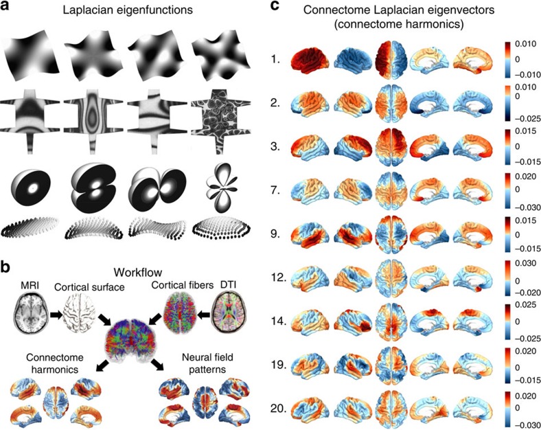
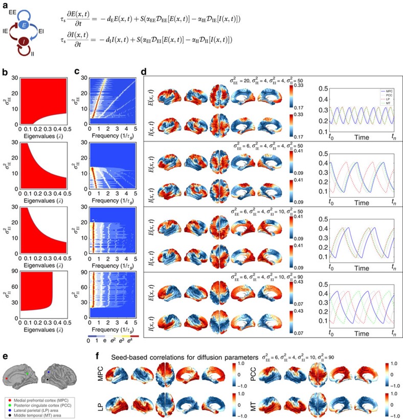
A key characteristic of human brain activity is coherent, spatially distributed oscillations forming behaviour-dependent brain networks. However, a fundamental principle underlying these networks remains unknown. Here we report that functional networks of the human brain are predicted by harmonic patterns, ubiquitous throughout nature, steered by the anatomy of the human cerebral cortex, the human connectome. We introduce a new technique extending the Fourier basis to the human connectome. In this new frequency-specific representation of cortical activity, that we call ‘connectome harmonics’, oscillatory networks of the human brain at rest match harmonic wave patterns of certain frequencies. We demonstrate a neural mechanism behind the self-organization of connectome harmonics with a continuous neural field model of excitatory–inhibitory interactions on the connectome. Remarkably, the critical relation between the neural field patterns and the delicate excitation–inhibition balance fits the neurophysiological changes observed during the loss and recovery of consciousness.
Overview
The claims and statistics of this paper haven’t been checked yet.
Free: it reads the open-access text and checks the first 5 claims that cite a source we can check. Create a free account to check every claim.
Integrity signals
Registry
Cites
Statistics
Figures



Verification
Claims the paper makes
The claims and statistics of this paper haven’t been checked yet.
Free: it reads the open-access text and checks the first 5 claims that cite a source we can check. Create a free account to check every claim.
Claims other papers make about this one
Each is checked against this paper’s own text: does it say what the citing paper says it does?
The source backs part of the claim, not all of it — or backs it for a different population, condition or comparison.
In the citing paper
“When this method was first introduced, Atasoy et al. (2016) compellingly demonstrated how reaction-diffusion simulations of spreading activation could generate resting state networks as stable modes—or standing waves—so recapitulating well-known patterns of neuronal organization with minimal assumptions.”
From An Integrated World Modeling Theory (IWMT) of Consciousness (2020) · cites this paper as Atasoy et al. (2016)
Experimental — accuracy not yet measured
Self-check
Percentages, sums and reported differences re-computed from the paper’s own numbers.
The self-check needs the paper’s full text.
Citations
Cites
Hodgkin, A. L., & Huxley, A. F. (1952) · The Journal of Physiology · doi:10.1113/jphysiol.1952.sp004764 · Cited by 23,191
The chemical basis of morphogenesis
Turing, A. M. (1952) · Philosophical Transactions of the Royal Society of London. Series B, Biological Sciences · doi:10.1098/rstb.1952.0012 · Cited by 11,733
The organization of the human cerebral cortex estimated by intrinsic functional connectivity
Thomas Yeo, B. T., Krienen, F. M., Sepulcre, J., Sabuncu, M. R., Lashkari, D., Hollinshead, M., Roffman, J. L., Smoller, J. W., Zöllei, L., Polimeni, J. R., et al. (2011) · Journal of Neurophysiology · doi:10.1152/jn.00338.2011 · Cited by 9,182
The human brain is intrinsically organized into dynamic, anticorrelated functional networks
Fox, M. D., Snyder, A. Z., Vincent, J. L., Corbetta, M., Van Essen, D. C., & Raichle, M. E. (2005) · Proceedings of the National Academy of Sciences · doi:10.1073/pnas.0504136102 · Cited by 8,553
The organization of the human cerebellum estimated by intrinsic functional connectivity
Buckner, R. L., Krienen, F. M., Castellanos, A., Diaz, J. C., & Yeo, B. T. T. (2011) · Journal of Neurophysiology · doi:10.1152/jn.00339.2011 · Cited by 7,304
Spontaneous fluctuations in brain activity observed with functional magnetic resonance imaging
Fox, M. D., & Raichle, M. E. (2007) · Nature Reviews Neuroscience · doi:10.1038/nrn2201 · Cited by 6,700
Neuronal Oscillations in Cortical Networks
Buzsáki, G., & Draguhn, A. (2004) · Science · doi:10.1126/science.1099745 · Cited by 6,576
Chung, F. (1996) · CBMS Regional Conference Series in Mathematics · doi:10.1090/cbms/092 · Cited by 5,524
Tracking whole-brain connectivity dynamics in the resting state
Allen, E. A., Damaraju, E., Plis, S. M., Erhardt, E. B., Eichele, T., & Calhoun, V. D. (2014) · Cerebral Cortex · doi:10.1093/cercor/bhs352 · Cited by 2,992
Dynamic functional connectivity: Promise, issues, and interpretations
Hutchison, R. M., Womelsdorf, T., Allen, E. A., Bandettini, P. A., Calhoun, V. D., Corbetta, M., Della Penna, S., Duyn, J. H., Glover, G. H., Gonzalez-Castillo, J., et al. (2013) · NeuroImage · doi:10.1016/j.neuroimage.2013.05.079 · Cited by 2,962
The general problem of the stability of motion
LYAPUNOV, A. M. (1992) · International Journal of Control · doi:10.1080/00207179208934253 · Cited by 2,550
Mathematical Biology: II: Spatial Models and Biomedical Applications
(2003) · Interdisciplinary Applied Mathematics · doi:10.1007/b98869 · Cited by 2,293
Spontaneous neuronal activity distinguishes human dorsal and ventral attention systems
Fox, M. D., Corbetta, M., Snyder, A. Z., Vincent, J. L., & Raichle, M. E. (2006) · Proceedings of the National Academy of Sciences · doi:10.1073/pnas.0604187103 · Cited by 2,101
NEURONAL CIRCUITS OF THE NEOCORTEX
Douglas, R. J., & Martin, K. A. C. (2004) · Annual Review of Neuroscience · doi:10.1146/annurev.neuro.27.070203.144152 · Cited by 1,886
A mathematical theory of the functional dynamics of cortical and thalamic nervous tissue
Wilson, H. R., & Cowan, J. D. (1973) · Kybernetik · doi:10.1007/bf00288786 · Cited by 1,850
An Undulatory Theory of the Mechanics of Atoms and Molecules
Schrödinger, E. (1926) · Physical Review · doi:10.1103/physrev.28.1049 · Cited by 1,826
Emerging concepts for the dynamical organization of resting-state activity in the brain
Deco, G., Jirsa, V. K., & McIntosh, A. R. (2011) · Nature reviews. Neuroscience · doi:10.1038/nrn2961 · Cited by 1,798
How Inhibition Shapes Cortical Activity
Isaacson, J. S., & Scanziani, M. (2011) · Neuron · doi:10.1016/j.neuron.2011.09.027 · Cited by 1,678
Reaction-Diffusion Model as a Framework for Understanding Biological Pattern Formation
Kondo, S., & Miura, T. (2010) · Science · doi:10.1126/science.1179047 · Cited by 1,651
Emergent complex neural dynamics
Chialvo, D. R. (2010) · Nature Physics · doi:10.1038/nphys1803 · Cited by 1,165
BOLD correlates of EEG topography reveal rapid resting-state network dynamics
Britz, J., Van De Ville, D., & Michel, C. M. (2010) · NeuroImage · doi:10.1016/j.neuroimage.2010.02.052 · Cited by 1,070
Large-scale model of mammalian thalamocortical systems
Izhikevich, E. M., & Edelman, G. M. (2008) · Proceedings of the National Academy of Sciences · doi:10.1073/pnas.0712231105 · Cited by 1,021
Britton, J. W., Sawyer, B. C., Keith, A. C., Wang, C.-C. J., Freericks, J. K., Uys, H., Biercuk, M. J., & Bollinger, J. J. (2012) · Nature · doi:10.1038/nature10981 · Cited by 941
On spurious and real fluctuations of dynamic functional connectivity during rest
Leonardi, N., & Van De Ville, D. (2015) · NeuroImage · doi:10.1016/j.neuroimage.2014.09.007 · Cited by 828
Laplace–Beltrami spectra as ‘Shape-DNA’ of surfaces and solids
Reuter, M., Wolter, F.-E., & Peinecke, N. (2006) · Computer-Aided Design · doi:10.1016/j.cad.2005.10.011 · Cited by 779
Nature and Interaction of Signals From the Receptive Field Center and Surround in Macaque V1 Neurons
Cavanaugh, J. R., Bair, W., & Movshon, J. A. (2002) · Journal of Neurophysiology · doi:10.1152/jn.00692.2001 · Cited by 778
Key role of coupling, delay, and noise in resting brain fluctuations
Deco, G., Jirsa, V., McIntosh, A. R., Sporns, O., & Kötter, R. (2009) · Proceedings of the National Academy of Sciences · doi:10.1073/pnas.0901831106 · Cited by 769
Time-resolved resting-state brain networks
Zalesky, A., Fornito, A., Cocchi, L., Gollo, L. L., & Breakspear, M. (2014) · Proceedings of the National Academy of Sciences · doi:10.1073/pnas.1400181111 · Cited by 753
A neural circuit for spatial summation in visual cortex
Adesnik, H., Bruns, W., Taniguchi, H., Huang, Z. J., & Scanziani, M. (2012) · Nature · doi:10.1038/nature11526 · Cited by 702
Temporal dynamics of spontaneous MEG activity in brain networks
de Pasquale, F., Della Penna, S., Snyder, A. Z., Lewis, C., Mantini, D., Marzetti, L., Belardinelli, P., Ciancetta, L., Pizzella, V., Romani, G. L., et al. (2010) · Proceedings of the National Academy of Sciences · doi:10.1073/pnas.0913863107 · Cited by 698
Decoupling of the brain's default mode network during deep sleep
Horovitz, S. G., Braun, A. R., Carr, W. S., Picchioni, D., Balkin, T. J., Fukunaga, M., & Duyn, J. H. (2009) · Proceedings of the National Academy of Sciences · doi:10.1073/pnas.0901435106 · Cited by 685
The Neural Correlates of Consciousness: An Update
Tononi, G., & Koch, C. (2008) · Annals of the New York Academy of Sciences · doi:10.1196/annals.1440.004 · Cited by 627
A mathematical theory of visual hallucination patterns
Ermentrout, G. B., & Cowan, J. D. (1979) · Biological Cybernetics · doi:10.1007/bf00336965 · Cited by 591
Ball, P. (2015) · Philosophical Transactions of the Royal Society B: Biological Sciences · doi:10.1098/rstb.2014.0218 · Cited by 590
Inhibition dominates sensory responses in the awake cortex
Haider, B., Häusser, M., & Carandini, M. (2013) · Nature · doi:10.1038/nature11665 · Cited by 539
Functional connectivity dynamics: modeling the switching behavior of the resting state
Hansen, E. C. A., Battaglia, D., Spiegler, A., Deco, G., & Jirsa, V. K. (2015) · NeuroImage · doi:10.1016/j.neuroimage.2014.11.001 · Cited by 528
Towards a theoretical foundation for Laplacian-based manifold methods
Belkin, M., & Niyogi, P. (2008) · Journal of Computer and System Sciences · doi:10.1016/j.jcss.2007.08.006 · Cited by 464
A Cortical Core for Dynamic Integration of Functional Networks in the Resting Human Brain
de Pasquale, F., Della Penna, S., Snyder, A. Z., Marzetti, L., Pizzella, V., Romani, G. L., & Corbetta, M. (2012) · Neuron · doi:10.1016/j.neuron.2012.03.031 · Cited by 420
Spatiotemporal dynamics of continuum neural fields
Bressloff, P. C. (2012) · Journal of Physics A: Mathematical and Theoretical · doi:10.1088/1751-8113/45/3/033001 · Cited by 414
Development of the Brain's Default Mode Network from Wakefulness to Slow Wave Sleep
Sämann, P. G., Wehrle, R., Hoehn, D., Spoormaker, V. I., Peters, H., Tully, C., Holsboer, F., & Czisch, M. (2011) · Cerebral Cortex · doi:10.1093/cercor/bhq295 · Cited by 399
Musso, F., Brinkmeyer, J., Mobascher, A., Warbrick, T., & Winterer, G. (2010) · NeuroImage · doi:10.1016/j.neuroimage.2010.01.093 · Cited by 387
Lateral competition for cortical space by layer-specific horizontal circuits
Adesnik, H., & Scanziani, M. (2010) · Nature · doi:10.1038/nature08935 · Cited by 356
Early and Late Mechanisms of Surround Suppression in Striate Cortex of Macaque
Webb, B. S., Dhruv, N. T., Solomon, S. G., Tailby, C., & Lennie, P. (2005) · The Journal of Neuroscience · doi:10.1523/jneurosci.3414-05.2005 · Cited by 334
A model for the formation of ocular dominance stripes
Swindale, N. V. (1980) · Proceedings of the Royal Society of London. Series B. Biological Sciences · doi:10.1098/rspb.1980.0051 · Cited by 244
How the Leopard Gets its Spots
Murray, J. D. (1988) · Scientific American · doi:10.1038/scientificamerican0388-80 · Cited by 237
Connectivity and Dynamics of Neural Information Processing
Jirsa, V. (2004) · Neuroinformatics · doi:10.1385/ni:2:2:183 · Cited by 140
Mexican hats and pinwheels in visual cortex
Kang, K., Shelley, M., & Sompolinsky, H. (2003) · Proceedings of the National Academy of Sciences · doi:10.1073/pnas.0138051100 · Cited by 136
Temporal oscillations in neuronal nets
Ermentrout, B., & Cowan, J. D. (1979) · Journal of Mathematical Biology · doi:10.1007/bf00275728 · Cited by 128
Dynamic causal modelling of distributed electromagnetic responses
Daunizeau, J., Kiebel, S. J., & Friston, K. J. (2009) · NeuroImage · doi:10.1016/j.neuroimage.2009.04.062 · Cited by 100
On nodes and modes in resting state fMRI
Friston, K. J., Kahan, J., Razi, A., Stephan, K. E., & Sporns, O. (2014) · NeuroImage · doi:10.1016/j.neuroimage.2014.05.056 · Cited by 85
Quantum Phase Extraction in Isospectral Electronic Nanostructures
Moon, C. R., Mattos, L. S., Foster, B. K., Zeltzer, G., Ko, W., & Manoharan, H. C. (2008) · Science · doi:10.1126/science.1151490 · Cited by 78
A Model for the Origin and Properties of Flicker-Induced Geometric Phosphenes
Rule, M. E., Stoffregen, M., & Ermentrout, B. (2011) · PLoS Computational Biology · doi:10.1371/journal.pcbi.1002158 · Cited by 76
Secondary Bifurcation in Neuronal Nets
Ermentrout, G. B., & Cowan, J. D. (1980) · SIAM Journal on Applied Mathematics · doi:10.1137/0139028 · Cited by 59
Spadone, S., de Pasquale, F., Mantini, D., & Penna, S. D. (2012) · NeuroImage · doi:10.1016/j.neuroimage.2012.05.051 · Cited by 27
Stewart, I. N. (1999) · Nature · doi:10.1038/44730 · Cited by 18
Holographic interferometry used to demonstrate a theory of pattern formation in animal coats
Xu, Y., Vest, C. M., & Murray, J. D. (1983) · Applied Optics · doi:10.1364/ao.22.003479 · Cited by 12
Physics, Emergence, and the Connectome
Laughlin, R. B. (2014) · Neuron · doi:10.1016/j.neuron.2014.08.006 · Cited by 8 · cited 1×
“where the adjacency matrix A is defined in equation (1) and”
BackgroundRoos, C. F. (2012) · Nature · doi:10.1038/484461a · Cited by 7
Basser (2000) · doi:10.1002/1522-2594(200010)44:4<625::aid-mrm17>3.0.co;2-o
Research works printed but not linked: 1
- Lévy, B. Laplace-Beltrami eigenfunctions towards an algorithm that “understands” geometry. In Int. Conf. Shape Modeling and Applications, 2006.
Cited by
Situating the default-mode network along a principal gradient of macroscale cortical organization
Margulies, D. S., Ghosh, S. S., Goulas, A., Falkiewicz, M., Huntenburg, J. M., Langs, G., Bezgin, G., Eickhoff, S. B., Castellanos, F. X., Petrides, M., et al. (2016) · Proceedings of the National Academy of Sciences · doi:10.1073/pnas.1608282113 · Cited by 2,321
Graph Signal Processing: Overview, Challenges, and Applications
Ortega, A., Frossard, P., Kovačević, J., Moura, J. M. F., & Vandergheynst, P. (2018) · Proceedings of the IEEE · doi:10.1109/jproc.2018.2820126 · Cited by 1,787
“imaging (fMRI) data [174], [175], [176].”
Large-Scale Gradients in Human Cortical Organization
Huntenburg, J. M., Bazin, P.-L., & Margulies, D. S. (2018) · Trends in Cognitive Sciences · doi:10.1016/j.tics.2017.11.002 · Cited by 968
Linking Structure and Function in Macroscale Brain Networks
Suárez, L. E., Markello, R. D., Betzel, R. F., & Misic, B. (2020) · Trends in Cognitive Sciences · doi:10.1016/j.tics.2020.01.008 · Cited by 764
“More recently, attention has shifted to decentralized mechanisms where signals diffuse through the network [56,57], often broadcast on multiple fronts [37,51,58,59].”
Lener, M. S., Niciu, M. J., Ballard, E. D., Park, M., Park, L. T., Nugent, A. C., & Zarate, C. A. (2017) · Biological Psychiatry · doi:10.1016/j.biopsych.2016.05.005 · Cited by 468
“Third, functional connectivity patterns within larger interconnected neural circuits have emerged from novel statistical techniques (60,61).”
Metadata
- Authors
- Atasoy, S., Donnelly, I., & Pearson, J.
- Affiliations
- UNSW Sydney (AU)
- Corresponding author
- Atasoy, Selen
- Venue
- Nature Communications
- Published
- 2016-01-21
- Volume
- 7
- Issue
- 1
- Pages
- 10340-10340
- ISSN
- 2041-1723 (ISSN-L)
- PMC
- PMC4735826
- OpenAlex
- W2267939148
- Cited by
- 381
- References
- 59
- Citations by year
- 2026: 38 · 2025: 50 · 2024: 40 · 2023: 55 · 2022: 39 · 2021: 50 · 2020: 39 · 2019: 25 · 2018: 18 · 2017: 19 · 2016: 8
- FWCI
- 14.85
- Type
- journal article
- Language
- en
- Open access
- gold
- doi.org
- Licence
- cc-by
- creativecommons.org/licenses/by/4.0 (tdm)
- creativecommons.org/licenses/by/4.0 (vor)
- Locations
- Nature Communications (publishedVersion, cc-by)
- PubMed Central (publishedVersion, cc-by)
- PubMed (publishedVersion)
- RePEc: Research Papers in Economics (submittedVersion)
- DOAJ (DOAJ: Directory of Open Access Journals) (submittedVersion, cc-by-sa)
- Funders
- National Institutes of Health (5u54mh091657-05)
- Australian Research Council (DP140101560)
- National Health and Medical Research Council (1049596, 1046198, 1024800, 1085404)
- National Institute of Mental Health (1U54 MH091657, U54-MH091657)
- Topics
- Life Sciences › Neuroscience › Cognitive Neuroscience › Neural dynamics and brain function
- Life Sciences › Neuroscience › Cognitive Neuroscience › Functional Brain Connectivity Studies
- Physical Sciences › Physics and Astronomy › Statistical and Nonlinear Physics › Nonlinear Dynamics and Pattern Formation
- Keywords
- human brain networks, functional connectivity, resting-state brain activity, neural field models, excitation-inhibition balance, self-organization, consciousness, cerebral cortex
- MeSH terms
- Adult, Brain, Brain Mapping, Female, Humans, Male, Nerve Net, Young Adult, Connectome
About these checks
Registry, retraction, Cites and statistics results are computed, not judged, with one exception: a printed reference that no index lists is read once by a model before it counts as a citation error. Claims are extracted by a model and kept only when their quote appears verbatim in the text; each cited source is then checked, with a model’s help, for whether it says what the claim relies on. Those verdicts can be wrong — read the claim’s quote and the cited source before relying on one.
Statistics and arithmetic are recomputed, not judged.
Confidence bands are shown only for fields calibrated on our annotated test set. None is calibrated yet, so no band is shown.
What counts as a claim ›How we measure confidence ›How we check this ›
Are you an author, or do you see a problem with this page? Request a review
Data sources
Bibliographic data: Semantic Scholar, OpenAlex, Crossref.
Contains information from the Semantic Scholar Academic Graph Datasets, made available under the ODC Attribution License (ODC-BY 1.0).
Semantic Scholar’s data is described in: Kinney, R., et al. (2023). The Semantic Scholar Open Data Platform. arXiv:2301.10140.
