

Face classification using electronic synapses
Open accessThe DOI matches its Crossref record; 33 of the 34 references it cites were found in a registry or an index.
Abstract
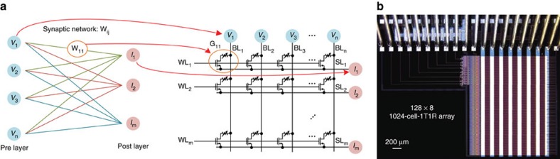
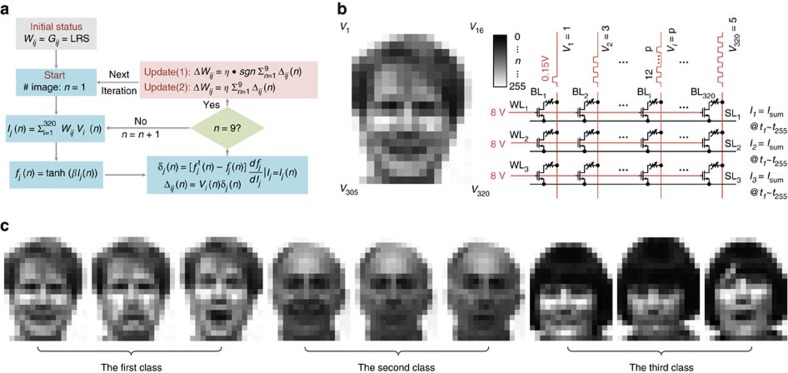
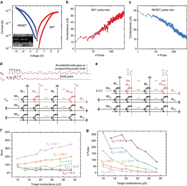
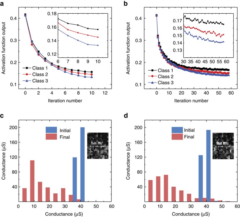
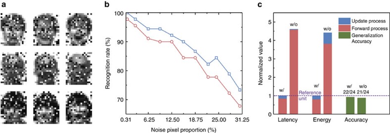
Conventional hardware platforms consume huge amount of energy for cognitive learning due to the data movement between the processor and the off-chip memory. Brain-inspired device technologies using analogue weight storage allow to complete cognitive tasks more efficiently. Here we present an analogue non-volatile resistive memory (an electronic synapse) with foundry friendly materials. The device shows bidirectional continuous weight modulation behaviour. Grey-scale face classification is experimentally demonstrated using an integrated 1024-cell array with parallel online training. The energy consumption within the analogue synapses for each iteration is 1,000 × (20 ×) lower compared to an implementation using Intel Xeon Phi processor with off-chip memory (with hypothetical on-chip digital resistive random access memory). The accuracy on test sets is close to the result using a central processing unit. These experimental results consolidate the feasibility of analogue synaptic array and pave the way toward building an energy efficient and large-scale neuromorphic system.
Overview
The claims and statistics of this paper haven’t been checked yet.
Free: it reads the open-access text and checks the first 5 claims that cite a source we can check. Create a free account to check every claim.
Integrity signals
Registry
Cites
Statistics
Figures
Verification
Claims the paper makes
The claims and statistics of this paper haven’t been checked yet.
Free: it reads the open-access text and checks the first 5 claims that cite a source we can check. Create a free account to check every claim.
Claims other papers make about this one
Each is checked against this paper’s own text: does it say what the citing paper says it does?
The cited source doesn’t support the claim as written.
In the citing paper
“the usual practice reported in the literature for this kind of training has been the use of the so-called Manhattan Update Rule105,194, or the Stochastic Gradient Descent54.”
From Hardware implementation of memristor-based artificial neural networks (2024) · cites this paper as [194]
Checked by a reasoning model — may be wrong.
Experimental — accuracy not yet measuredThe source backs part of the claim, not all of it — or backs it for a different population, condition or comparison.
In the citing paper
“leading to a variety of prototypes in which the circuitry needed for the backpropagation are implemented off-chip, an approach here labelled as partial-in situ. This is the case of refs. 54,105,194.”
From Hardware implementation of memristor-based artificial neural networks (2024) · cites this paper as [194]
Experimental — accuracy not yet measuredThe source backs part of the claim, not all of it — or backs it for a different population, condition or comparison.
In the citing paper
“In all these works the VMM operation required for the forward pass is performed by the memristor crossbar and the digitalized output vectors recorded by an acquisition printed circuit board. Then the output vector is processed by the training algorithm in software to determine how to update the synaptic weight after each training epoch.”
From Hardware implementation of memristor-based artificial neural networks (2024) · cites this paper as [194]
Experimental — accuracy not yet measuredThe source backs part of the claim, not all of it — or backs it for a different population, condition or comparison.
In the citing paper
“The most elementary approach is a sequential (row-by-row) analogue multiplication with binary inputs194, which does not perform an analogue VMM operation because, despite the multiplication operation is done in each memristor, the accumulation is performed by external circuitry.”
From Hardware implementation of memristor-based artificial neural networks (2024) · cites this paper as [194]
Experimental — accuracy not yet measuredThe cited source says what the claim attributes to it.
In the citing paper
“Some groups prefer to incorporate a transistor in series to each MIM cell to obtain a better control over the currents through the device (i.e., improve conductance controllability and minimize sneak path currents)53–55,60,61,102,113,167,194,218–222,).”
From Hardware implementation of memristor-based artificial neural networks (2024) · cites this paper as [194]
Self-check
Percentages, sums and reported differences re-computed from the paper’s own numbers.
The self-check needs the paper’s full text.
Citations
Cites
Gradient-based learning applied to document recognition
Lecun, Y., Bottou, L., Bengio, Y., & Haffner, P. (1998) · Proceedings of the IEEE · doi:10.1109/5.726791 · Cited by 58,805
ImageNet Large Scale Visual Recognition Challenge
Russakovsky, O., Deng, J., Su, H., Krause, J., Satheesh, S., Ma, S., Huang, Z., Karpathy, A., Khosla, A., Bernstein, M., et al. (2015) · International Journal of Computer Vision · doi:10.1007/s11263-015-0816-y · Cited by 39,380
Human-level control through deep reinforcement learning
Mnih, V., Kavukcuoglu, K., Silver, D., Rusu, A. A., Veness, J., Bellemare, M. G., Graves, A., Riedmiller, M., Fidjeland, A. K., Ostrovski, G., et al. (2015) · Nature · doi:10.1038/nature14236 · Cited by 30,357
Reducing the dimensionality of data with neural networks
Hinton, G. E., & Salakhutdinov, R. R. (2006) · Science · doi:10.1126/science.1127647 · Cited by 20,928
The perceptron: A probabilistic model for information storage and organization in the brain.
Rosenblatt, F. (1958) · Psychological Review · doi:10.1037/h0042519 · Cited by 12,280
Eigenfaces vs. Fisherfaces: recognition using class specific linear projection
Belhumeur, P. N., Hespanha, J. P., & Kriegman, D. J. (1997) · IEEE Transactions on Pattern Analysis and Machine Intelligence · doi:10.1109/34.598228 · Cited by 11,707
A million spiking-neuron integrated circuit with a scalable communication network and interface
Merolla, P. A., Arthur, J. V., Alvarez-Icaza, R., Cassidy, A. S., Sawada, J., Akopyan, F., Jackson, B. L., Imam, N., Guo, C., Nakamura, Y., et al. (2014) · Science · doi:10.1126/science.1254642 · Cited by 4,147
Training and operation of an integrated neuromorphic network based on metal-oxide memristors
Prezioso, M., Merrikh-Bayat, F., Hoskins, B. D., Adam, G. C., Likharev, K. K., & Strukov, D. B. (2015) · Nature · doi:10.1038/nature14441 · Cited by 3,001 · cited 3×
“Meanwhile, pattern recognition tasks based on analogue resistive random access memory (RRAM) have been demonstrated either through simulations or on a small crossbar array 13,14 .”
BackgroundMethodWong, H.-S. P., Lee, H.-Y., Yu, S., Chen, Y.-S., Wu, Y., Chen, P.-S., Lee, B., Chen, F. T., & Tsai, M.-J. (2012) · Proceedings of the IEEE · doi:10.1109/jproc.2012.2190369 · Cited by 2,757
Self-citationDeep learning applications and challenges in big data analytics
Najafabadi, M. M., Villanustre, F., Khoshgoftaar, T. M., Seliya, N., Wald, R., & Muharemagic, E. (2015) · Journal of Big Data · doi:10.1186/s40537-014-0007-7 · Cited by 2,594
Research works printed but not linked: 6
- Le, Q. V. in Acoustics, Speech and Signal Processing (ICASSP), 2013 IEEE International Conference 8595–8598 (IEEE, 2013).
- Krizhevsky, A., Sutskever, I. & Hinton, G. E. in Advances in Neural Information Processing Systems 1097–1105 (Curran Associates, Inc., 2012).
- Fackenthal, R. et al. in Solid-State Circuits Conference Digest of Technical Papers (ISSCC), 2014 IEEE International, 338–339 (IEEE, 2014).
- Govoreanu, B. et al. in Electron Devices Meeting (IEDM), 2011 IEEE International, 31.36. 31–31.36. 34 (IEEE, 2011).
- Sekar, D. et al. in 2014 IEEE International Electron Devices Meeting, 28.23. 21–28.23. 24 (IEEE, 2014).
- Burr, G. et al. in 2015 IEEE International Electron Devices Meeting (IEDM), 4.4. 1–4.4. 4 (IEEE, 2015).
Cited by
Items 201–300 of 918
Lin, Y., Zeng, T., Xu, H., Wang, Z., Zhao, X., Liu, W., Ma, J., & Liu, Y. (2018) · Advanced Electronic Materials · doi:10.1002/aelm.201800373 · Cited by 85
Echo state graph neural networks with analogue random resistive memory arrays
Wang, S., Li, Y., Wang, D., Zhang, W., Chen, X., Dong, D., Wang, S., Zhang, X., Lin, P., Gallicchio, C., et al. (2023) · Nature Machine Intelligence · doi:10.1038/s42256-023-00609-5 · Cited by 84
Self-citationEmerging memory technologies for neuromorphic computing
Kim, C.-H., Lim, S., Woo, S. Y., Kang, W.-M., Seo, Y.-T., Lee, S., Lee, S., Kwon, D., Oh, S., Noh, Y., et al. (2018) · Nanotechnology · doi:10.1088/1361-6528/aae975 · Cited by 91
Light-Emitting Memristors for Optoelectronic Artificial Efferent Nerve
Zhu, Y., Wu, C., Xu, Z., Yang, L., Hu, H., Guo, T., Kim, T. W., Chai, Y., & Li, F. (2021) · Nano Letters · doi:10.1021/acs.nanolett.1c01482 · Cited by 83
Ultrathin Nitride Ferroic Memory with Large ON/OFF Ratios for Analog In‐Memory Computing
Wang, D., Wang, P., Mondal, S., Hu, M., Wu, Y., Ma, T., & Mi, Z. (2023) · Advanced Materials · doi:10.1002/adma.202210628 · Cited by 83
Ismail, M., Rasheed, M., Mahata, C., Kang, M., & Kim, S. (2023) · Nano Convergence · doi:10.1186/s40580-023-00380-8 · Cited by 83
Computing with ferroelectric FETs: Devices, models, systems, and applications
Aziz, A., Breyer, E. T., Chen, A., Chen, X., Datta, S., Gupta, S. K., Hoffmann, M., Hu, X. S., Ionescu, A. M., Jerry, M., et al. (2018) · Design, Automation, and Test in Europe · doi:10.23919/date.2018.8342213 · Cited by 91
Evidence of soft bound behaviour in analogue memristive devices for neuromorphic computing
Frascaroli, J., Brivio, S., Covi, E., & Spiga, S. (2018) · Scientific Reports · doi:10.1038/s41598-018-25376-x · Cited by 88
Artificial Neural Networks Based on Memristive Devices: From Device to System
Huang, H.-M., Wang, Z., Wang, T., Xiao, Y., & Guo, X. (2020) · Advanced Intelligent Systems · doi:10.1002/aisy.202000149 · Cited by 82
Broadband Visual Adaption and Image Recognition in a Monolithic Neuromorphic Machine Vision System
Cai, Y., Wang, F., Wang, X., Li, S., Wang, Y., Yang, J., Yan, T., Zhan, X., Wang, F., Cheng, R., et al. (2022) · Advanced Functional Materials · doi:10.1002/adfm.202212917 · Cited by 82
Unsupervised Learning on Resistive Memory Array Based Spiking Neural Networks
Guo, Y., Wu, H., Gao, B., & Qian, H. (2019) · Frontiers in Neuroscience · doi:10.3389/fnins.2019.00812 · Cited by 79
Self-citationWang, C., Li, Y., Wang, Y., Xu, X., Fu, M., Liu, Y., Lin, Z., Ling, H., Gkoupidenis, P., Yi, M., et al. (2021) · Journal of Materials Chemistry C · doi:10.1039/d1tc01660a · Cited by 80
Signal Filtering Enabled by Spike Voltage‐Dependent Plasticity in Metalloporphyrin‐Based Memristors
Wang, Z., Wang, L., Wu, Y. H., Bian, L., Nagai, M., Jv, R., Xie, L., Ling, H., Li, Q., Bian, H., et al. (2021) · Advanced Materials · doi:10.1002/adma.202104370 · Cited by 78
A Memristor‐Based Silicon Carbide for Artificial Nociceptor and Neuromorphic Computing
Liu, L., Zhao, J., Cao, G., Zheng, S., & Yan, X. (2021) · Advanced Materials Technologies · doi:10.1002/admt.202100373 · Cited by 79
In-memory computing with emerging nonvolatile memory devices
Cheng, C., Tiw, P. J., Cai, Y., Yan, X., Yang, Y., & Huang, R. (2021) · Science China Information Sciences · doi:10.1007/s11432-021-3327-7 · Cited by 77
Huh, W., Lee, D., Jang, S., Kang, J. H., Yoon, T. H., So, J., Kim, Y. H., Kim, J. C., Park, H., Jeong, H. Y., et al. (2023) · Advanced Materials · doi:10.1002/adma.202211525 · Cited by 80
Strategies to Improve the Accuracy of Memristor-Based Convolutional Neural Networks
Pan, W.-Q., Chen, J., Kuang, R., Li, Y., He, Y.-H., Feng, G.-R., Duan, N., Chang, T.-C., & Miao, X.-S. (2020) · IEEE Transactions on Electron Devices · doi:10.1109/ted.2019.2963323 · Cited by 76
Opto-electronic memristors: Prospects and challenges in neuromorphic computing
Emboras, A., Alabastri, A., Lehmann, P., Portner, K., Weilenmann, C., Ma, P., Cheng, B., Lewerenz, M., Passerini, E., Koch, U., et al. (2020) · Applied Physics Letters · doi:10.1063/5.0028539 · Cited by 78
Kim, K., Song, M. S., Hwang, H., Hwang, S., & Kim, H. (2024) · Frontiers in Neuroscience · doi:10.3389/fnins.2024.1279708 · Cited by 81
Sign backpropagation: An on-chip learning algorithm for analog RRAM neuromorphic computing systems
Zhang, Q., Wu, H., Yao, P., Zhang, W., Gao, B., Deng, N., & Qian, H. (2018) · Neural Networks · doi:10.1016/j.neunet.2018.08.012 · Cited by 75
Self-citationAssociative Memory for Image Recovery with a High‐Performance Memristor Array
Zhou, Y. C., Wu, H., Gao, B., Wu, W., Xi, Y., Yao, P., Zhang, S., Zhang, Q., & Qian, H. (2019) · Advanced Functional Materials · doi:10.1002/adfm.201900155 · Cited by 76
Self-citationIn-memory computing to break the memory wall*
Huang, X., Liu, C., Jiang, Y., & Zhou, P. (2020) · Chinese Physics B · doi:10.1088/1674-1056/ab90e7 · Cited by 79
Self-citationHfO x /AlO y Superlattice‐Like Memristive Synapse
Wang, C., Mao, G., Huang, M., Huang, E., Zhang, Z., Yuan, J., Cheng, W., Xue, K., Wang, X., & Miao, X. (2022) · Advanced Science · doi:10.1002/advs.202201446 · Cited by 91
Gate-Tunable Synaptic Dynamics of Ferroelectric-Coupled Carbon-Nanotube Transistors
Choi, Y., Kim, J. H., Qian, C., Kang, J., Hersam, M. C., Park, J., & Cho, J. H. (2019) · ACS Applied Materials & Interfaces · doi:10.1021/acsami.9b17742 · Cited by 73
Nanoscale memristor devices: materials, fabrication, and artificial intelligence
Yu, Y., Xiao, M., Fieser, D., Zhou, W., & Hu, A. (2024) · Journal of Materials Chemistry C · doi:10.1039/d3tc04510b · Cited by 78
Quantitative, Dynamic TaO x Memristor/Resistive Random Access Memory Model
Lee, S. H., Moon, J., Jeong, Y., Lee, J., Li, X., Wu, H., & Lu, W. D. (2020) · ACS Applied Electronic Materials · doi:10.1021/acsaelm.9b00792 · Cited by 72
Self-citationLi, H., Huang, X., Yuan, J., Lu, Y., Wan, T., Li, Y., Xue, K., He, Y., Xu, M., Tong, H., et al. (2020) · Advanced Electronic Materials · doi:10.1002/aelm.202000309 · Cited by 74
Self-citationFPSA: A Full System Stack Solution for Reconfigurable ReRAM-based NN Accelerator Architecture
Ji, Y., Zhang, Y., Xie, X., Li, S., Wang, P., Hu, X., Zhang, Y., & Xie, Y. (2019) · International Conference on Architectural Support for Programming Languages and Operating Systems (ASPLOS) · doi:10.1145/3297858.3304048 · Cited by 79
Phase Change Random Access Memory for Neuro‐Inspired Computing
Wang, Q., Niu, G., Ren, W., Wang, R., Chen, X.-G., Li, X., Ye, Z., Xie, Y., Song, S., & Song, Z. (2021) · Advanced Electronic Materials · doi:10.1002/aelm.202001241 · Cited by 74
Multi-state MRAM cells for hardware neuromorphic computing
Rzeszut, P., Chęciński, J., Brzozowski, I., Ziętek, S., Skowroński, W., & Stobiecki, T. (2022) · Scientific Reports · doi:10.1038/s41598-022-11199-4 · Cited by 78
Toward memristive in-memory computing: principles and applications
Bao, H., Zhou, H., Li, J., Pei, H.-Z., Tian, J., Yang, L., Ren, S., Tong, S.-Q., Li, Y., He, Y., et al. (2022) · Frontiers of Optoelectronics · doi:10.1007/s12200-022-00025-4 · Cited by 79
Self-citationKuang, J., Liu, K., Liu, M., Shao, M., Zhu, M., Liu, G., Wen, W., Chen, J., Qin, M., Pan, Z., et al. (2022) · Advanced Functional Materials · doi:10.1002/adfm.202209502 · Cited by 71
Zhang, T., Guo, X., Wang, P., Fan, X., Wang, Z., Tong, Y., Wang, D., Tong, L., & Li, L. (2024) · Nature Communications · doi:10.1038/s41467-024-46867-8 · Cited by 73
In situ training of an in-sensor artificial neural network based on ferroelectric photosensors
Lin, H., Ou, J., Fan, Z. H., Yan, X., Hu, W., Cui, B., Xu, J., Li, W., Chen, Z., Yang, B., et al. (2025) · Nature Communications · doi:10.1038/s41467-024-55508-z · Cited by 69
Jang, J., Gi, S., Yeo, I., Choi, S., Jang, S., Ham, S., Lee, B., & Wang, G. (2022) · Advanced Science · doi:10.1002/advs.202201117 · Cited by 68
Spontaneous sparse learning for PCM-based memristor neural networks
Lim, D., Wu, S., Zhao, R. J., Lee, J.-H., Jeong, H., & Shi, L. (2021) · Nature Communications · doi:10.1038/s41467-020-20519-z · Cited by 76
Self-citationLiSiOX-Based Analog Memristive Synapse for Neuromorphic Computing
Chen, J., Lin, C.-Y., Li, Y., Qin, C., Lu, K., Wang, J., Chen, C.-K., He, Y., Chang, T., Sze, S. M., et al. (2019) · IEEE Electron Device Letters · doi:10.1109/led.2019.2898443 · Cited by 71
A memristive deep belief neural network based on silicon synapses
Wang, W., Danial, L., Li, Y., Herbelin, E., Pikhay, E., Roizin, Y., Hoffer, B., Wang, Z., & Kvatinsky, S. (2022) · Nature Electronics · doi:10.1038/s41928-022-00878-9 · Cited by 66
Byun, K., Choi, I., Kwon, S., Kim, Y., Kang, D., Cho, Y. W., Yoon, S. K., & Kim, S. (2022) · Advanced Materials Technologies · doi:10.1002/admt.202200884 · Cited by 68
Conductive-bridging random-access memories for emerging neuromorphic computing
Cha, J., Yang, S. Y., Oh, J., Choi, S., Park, S., Jang, B. C., Ahn, W., & Choi, S. (2020) · Nanoscale · doi:10.1039/d0nr01671c · Cited by 67
Gao, B., Wu, H., Wu, W., Wang, X., Yao, P., Xi, Y., Zhang, W., Deng, N., Huang, P. C., Liu, X., et al. (2017) · Technical digest - International Electron Devices Meeting/Technical digest · doi:10.1109/iedm.2017.8268326 · Cited by 65
Self-citationPiezotronic Synapse Based on a Single GaN Microwire for Artificial Sensory Systems
Hua, Q., Cui, X. Y., Liu, H., Pan, C., Hu, W., & Wang, Z. L. (2020) · Nano Letters · doi:10.1021/acs.nanolett.0c00733 · Cited by 66
Zhou, X. Y., Zhao, L., Zhen, W., Lin, Y., Wang, C., Pan, T., Li, L., Du, G., Lu, L., Cao, X., et al. (2021) · Advanced Electronic Materials · doi:10.1002/aelm.202001254 · Cited by 64
Kim, S., Park, J., Kim, T., Hong, K., Hwang, Y., Park, B., & Kim, H. (2022) · Advanced Intelligent Systems · doi:10.1002/aisy.202100273 · Cited by 65
Xu, Y., Shi, Y., Qian, C., Xie, P., Jin, C., Shi, X., Zhang, G., Liu, W., Wan, C., Ho, J. C. Y., et al. (2023) · Nano Letters · doi:10.1021/acs.nanolett.3c01291 · Cited by 64
Fang, J., Tang, Z., Lai, X.-C., Qiu, F., Jiang, Y., Liu, Q., Tang, X., Sun, Q., Zhou, Y., Fan, J., et al. (2024) · ACS Applied Materials & Interfaces · doi:10.1021/acsami.4c05316 · Cited by 64
Review of Memristors for In‐Memory Computing and Spiking Neural Networks
Shooshtari, M., Serrano‐Gotarredona, T., & Linares‐Barranco, B. (2025) · Advanced Intelligent Systems · doi:10.1002/aisy.202500806 · Cited by 74
An Attention-Based Spiking Neural Network for Unsupervised Spike-Sorting
Bernert, M., & Yvert, B. (2018) · International Journal of Neural Systems · doi:10.1142/s0129065718500594 · Cited by 66
Design and optimization of FeFET-based crossbars for binary convolution neural networks
Chen, X., Yin, X., Niemier, M. T., & Hu, X. S. (2018) · Design, Automation, and Test in Europe · doi:10.23919/date.2018.8342199 · Cited by 70
In-Memory Computing with Memristor Arrays
Li, C., Belkin, D., Li, Y., Yan, P., Hu, M., Ge, N., Jiang, H., Montgomery, E., Lin, P., Wang, Z., et al. (2018) · IEEE International Memory Workshop (IMW) · doi:10.1109/imw.2018.8388838 · Cited by 63
Ziegler, M., Wenger, C., Chicca, E., & Kohlstedt, H. (2018) · Journal of Applied Physics · doi:10.1063/1.5042040 · Cited by 66
Realizing Scalable Two-Dimensional MoS2Synaptic Devices for Neuromorphic Computing
Lee, E., Kim, J., Bhoyate, S. D., Cho, K., & Choi, W. (2020) · Chemistry of Materials · doi:10.1021/acs.chemmater.0c03112 · Cited by 62
Recent Progress in Neuromorphic Computing from Memristive Devices to Neuromorphic Chips
Xiao, Y., Gao, C., Jin, J., Sun, W., Wang, B., Bao, Y., Liu, C., Huang, W., Zeng, H., & Yu, Y. (2024) · Advanced Devices & Instrumentation · doi:10.34133/adi.0044 · Cited by 68
A System-Level Simulator for RRAM-Based Neuromorphic Computing Chips
Lee, M. K. F., Cui, Y., Somu, T., Luo, T., Zhou, J. R., Tang, W. T., Wong, W., & Goh, R. S. M. (2018) · ACM Transactions on Architecture and Code Optimization · doi:10.1145/3291054 · Cited by 62
Trends and challenges in the circuit and macro of RRAM-based computing-in-memory systems
Wei, S.-T., Gao, B., Wu, D. M., Tang, J., Qian, H., & Wu, H. (2022) · Chip · doi:10.1016/j.chip.2022.100004 · Cited by 61
Self-citationLi, H., Geng, S., Liu, T., Cao, M., & Su, J. (2023) · ACS Applied Materials & Interfaces · doi:10.1021/acsami.2c19836 · Cited by 62
Lee, D. H., Lim, T., Pyeon, J., Park, H., Lee, S., Lee, S., Kim, W., Kim, M. S., Lee, J., Kim, D., et al. (2024) · Advanced Materials · doi:10.1002/adma.202310956 · Cited by 66
Tailoring synaptic plasticity in a perovskite QD-based asymmetric memristor
Gong, Y., Wang, Y., Li, R., Yang, J., Lv, Z., Xing, X., Liao, Q., Wang, J., Chen, J., Zhou, Y., et al. (2020) · Journal of Materials Chemistry C · doi:10.1039/c9tc06565b · Cited by 61
Lee, E., Kim, J., Park, J., Hwang, J., Jang, H., Cho, K., & Choi, W. (2023) · ACS Applied Materials & Interfaces · doi:10.1021/acsami.2c21688 · Cited by 60
An Electromagnetic Perspective of Artificial Intelligence Neuromorphic Chips
Li, E., Ma, H., Ahmed, M., Tao, T., Gu, Z., Chen, M., Chen, Q., Li, D., & Chen, W. (2023) · Electromagnetic Science · doi:10.23919/emsci.2023.0015 · Cited by 65
Memristive Ion Dynamics to Enable Biorealistic Computing
Zhao, R., Kim, S. J., Xu, Y., Zhao, J., Wang, T., Midya, R., Ganguli, S., Roy, A. K., Dubey, M., Williams, R. S., et al. (2024) · Chemical Reviews · doi:10.1021/acs.chemrev.4c00587 · Cited by 61
Kim, H., Oh, S., Choo, H., Kang, D., & Park, J. (2023) · ACS Nano · doi:10.1021/acsnano.3c05337 · Cited by 60
Oxygen-Migration-Based Spintronic Device Emulating a Biological Synapse
Mishra, R., Kumar, D., & Yang, H. (2019) · Physical Review Applied · doi:10.1103/physrevapplied.11.054065 · Cited by 59
Dopamine-like STDP modulation in nanocomposite memristors
Nikiruy, K. E., Emelyanov, A. V., Demin, V. A., Ситников, А. В., Minnekhanov, A. A., Rylkov, V. V., Kashkarov, P. K., & Kovalchuk, M. V. (2019) · AIP Advances · doi:10.1063/1.5111083 · Cited by 59
Threshold Switching in Single Metal‐Oxide Nanobelt Devices Emulating an Artificial Nociceptor
Xiao, M. W., Shen, D., Futscher, M. H., Ehrler, B., Musselman, K. P., Duley, W. W., & Zhou, Y. (2019) · Advanced Electronic Materials · doi:10.1002/aelm.201900595 · Cited by 59
Choi, S. C., Kim, Y. Y., Nguyen, T. V., Jeong, W. H., Min, K., & Choi, B. J. (2021) · Advanced Electronic Materials · doi:10.1002/aelm.202100050 · Cited by 64
Recent advances in neuromorphic transistors for artificial perception applications
Wang, W. S., & Zhu, L. Q. (2022) · Science and Technology of Advanced Materials · doi:10.1080/14686996.2022.2152290 · Cited by 58
Zhao, Y., Lou, Z., Hu, J., Li, Z., Xu, L., Chen, Z., Xu, Z., Wang, T., Wu, M., Ying, H., et al. (2024) · Advanced Materials · doi:10.1002/adma.202406608 · Cited by 58
An overview of critical applications of resistive random access memory
Zahoor, F., Nisar, A., Bature, U. I., Abbas, H., Bashir, F. I., Chattopadhyay, A., Kaushik, B. K., Alzahrani, A., & Hussin, F. A. (2024) · Nanoscale Advances · doi:10.1039/d4na00158c · Cited by 60
Unsupervised Hebbian learning experimentally realized with analogue memristive crossbar arrays
Hansen, M., Zahari, F., Kohlstedt, H., & Ziegler, M. (2018) · Scientific Reports · doi:10.1038/s41598-018-27033-9 · Cited by 66
Wang, T., Meng, J., He, Z., Chen, L., Zhu, H., Sun, Q., Ding, S., & Zhang, D. W. (2019) · Nanoscale Research Letters · doi:10.1186/s11671-019-2933-y · Cited by 57
Lin, Y., Wang, C., Ren, Y., Wang, Z., Xu, H., Zhao, X., Ma, J., & Liu, Y. (2019) · Small Methods · doi:10.1002/smtd.201900160 · Cited by 57
Berco, D., & Ang, D. S. (2019) · Advanced Intelligent Systems · doi:10.1002/aisy.201900003 · Cited by 58
Memristor-based LSTM network with in situ training and its applications
Liu, X., Zeng, Z., & Wunsch, D. C. (2020) · Neural Networks · doi:10.1016/j.neunet.2020.07.035 · Cited by 60
Memristor-based signal processing for edge computing
Zhao, H., Liu, Z., Tang, J., Gao, B., Zhang, Y., Qian, H., & Wu, H. (2021) · Tsinghua Science & Technology · doi:10.26599/tst.2021.9010043 · Cited by 56
Self-citationA self-adaptive hardware with resistive switching synapses for experience-based neurocomputing
Bianchi, S., Muñoz-Martín, I., Covi, E., Bricalli, A., Piccolboni, G., Regev, A., Molas, G., Nodin, J. F., Andrieu, F., & Ielmini, D. (2023) · Nature Communications · doi:10.1038/s41467-023-37097-5 · Cited by 58
Recent advances in ferroelectric materials, devices, and in-memory computing applications
Hwang, H., Youn, S., & Kim, H. (2025) · Nano Convergence · doi:10.1186/s40580-025-00520-2 · Cited by 58
Wang, J., Hu, S., Zhan, X., Yu, Q., Liu, Z., Chen, T. P., Yin, Y., Hosaka, S., & Liu, Y. (2018) · Scientific Reports · doi:10.1038/s41598-018-30768-0 · Cited by 55
Mixed size crossbar based RRAM CNN accelerator with overlapped mapping method
Zhu, Z., Lin, J., Cheng, M., Xia, L., Sun, H., Chen, X., Wang, Y., & Yang, H. (2018) · doi:10.1145/3240765.3240825 · Cited by 55
Li, J., Yang, Y., Yin, M., Sun, X., Li, L., & Huang, R. (2020) · Materials Horizons · doi:10.1039/c9mh01206k · Cited by 54
Wang, Q., Zhao, C., Sun, Y., Xu, R., Li, C., Wang, C., Liu, W., Gu, J., Shi, Y., Yang, L., et al. (2023) · Microsystems & Nanoengineering · doi:10.1038/s41378-023-00566-4 · Cited by 55
Multi-level resistive switching in hafnium-oxide-based devices for neuromorphic computing
Hellenbrand, M., & MacManus‐Driscoll, J. L. (2023) · Nano Convergence · doi:10.1186/s40580-023-00392-4 · Cited by 57
Design Guidelines of RRAM based Neural-Processing-Unit: A Joint Device-Circuit-Algorithm Analysis
Zhang, W., Peng, X., Wu, H., Gao, B., He, H., Zhang, Y., Yu, S., & Qian, H. (2019) · ACM/IEEE Design Automation Conference (DAC) · doi:10.1145/3316781.3317797 · Cited by 54
Self-citationLi, Z., Tian, B., Xue, K., Wang, B., Xu, M., Lu, H., Sun, H., & Miao, X. (2019) · IEEE Electron Device Letters · doi:10.1109/led.2019.2917935 · Cited by 54
A Compact Model of Analog RRAM With Device and Array Nonideal Effects for Neuromorphic Systems
Liao, Y., Gao, B., Xu, F., Yao, P., Chen, J., Zhang, W., Tang, J., Wu, H., & Qian, H. (2020) · IEEE Transactions on Electron Devices · doi:10.1109/ted.2020.2975314 · Cited by 53
Self-citationRecent advances in curved image sensor arrays for bioinspired vision system
Gao, W., Xu, Z., Han, X., & Pan, C. (2021) · Nano Today · doi:10.1016/j.nantod.2021.101366 · Cited by 54
Emerging memristive artificial neuron and synapse devices for the neuromorphic electronics era
Li, J., Abbas, H., Ang, D. S., Ali, A., & Ju, X. (2023) · Nanoscale Horizons · doi:10.1039/d3nh00180f · Cited by 56
A Ti/AlOx/TaOx/Pt Analog Synapse for Memristive Neural Network
Sun, Y. K., Xu, H. F., Wang, C., Song, B., Liu, H., Liu, Q., Liu, S., & Li, Q. (2018) · IEEE Electron Device Letters · doi:10.1109/led.2018.2860053 · Cited by 59
Optoelectronic memristor for neuromorphic computing*
Xue, W., Ci, W., Xu, X., & Liu, G. (2020) · Chinese Physics B · doi:10.1088/1674-1056/ab75da · Cited by 53
Shen, J., Zhou, B., Wang, F., Wan, Q. C., Shan, X., Li, C., Lin, X., & Zhang, K. (2020) · Nanotechnology · doi:10.1088/1361-6528/ab82d6 · Cited by 53
Du, N., Schmidt, H., & Polian, I. (2021) · Nano Materials Science · doi:10.1016/j.nanoms.2021.01.001 · Cited by 57
Multi-State Memristors and Their Applications: An Overview
Wang, C., Si, Z., Jiang, X., Malik, A., Pan, Y., Stathopoulos, S., Serb, A., Wang, S., Prodromakis, T., & Papavassiliou, C. (2022) · IEEE Journal on Emerging and Selected Topics in Circuits and Systems · doi:10.1109/jetcas.2022.3223295 · Cited by 54
Xiang, Y., Huang, P. C., Zhao, Y., Zhao, M., Gao, B., Wu, H., Qian, H., Liu, X., & Kang, J. (2019) · IEEE Transactions on Electron Devices · doi:10.1109/ted.2019.2931135 · Cited by 56
Self-citationChen, Y., Lin, C., Hu, S.-T., Lin, C., Fowler, B. W., & Lee, J. (2019) · Scientific Reports · doi:10.1038/s41598-019-48932-5 · Cited by 52
Sparse Attention Acceleration with Synergistic In-Memory Pruning and On-Chip Recomputation
Yazdanbakhsh, A., Moradifirouzabadi, A., Li, Z., & Kang, M. (2022) · IEEE/ACM International Symposium on Microarchitecture (MICRO) · doi:10.1109/micro56248.2022.00059 · Cited by 63
Optically modulated electric synapses realized with memristors based on ZnO nanorods
Zhou, W., Yang, R., He, H., Huang, H.-M., Xiong, J., & Guo, X. (2018) · Applied Physics Letters · doi:10.1063/1.5045643 · Cited by 51
Technological Benchmark of Analog Synaptic Devices for Neuroinspired Architectures
Chen, P.-Y., & Yu, S. (2018) · IEEE Design and Test · doi:10.1109/mdat.2018.2890229 · Cited by 52
Integrated Memristor Network for Physiological Signal Processing
Cai, L., Yu, L., Yue, W., Zhu, Y., Yang, Z., Li, Y., Tao, Y., & Yang, Y. (2023) · Advanced Electronic Materials · doi:10.1002/aelm.202300021 · Cited by 50
Synaptic Resistors for Concurrent Inference and Learning with High Energy Efficiency
Danesh, C., Shaffer, C. M., Nathan, D., Shenoy, R., Tudor, A., Tadayon, M., Lin, Y., & Chen, Y. (2019) · Advanced Materials · doi:10.1002/adma.201808032 · Cited by 54
Woo, J., & Yu, S. (2019) · IEEE Transactions on Very Large Scale Integration (VLSI) Systems · doi:10.1109/tvlsi.2019.2917764 · Cited by 52
Metadata
- Authors
- Yao, P., Wu, H., Gao, B., Eryilmaz, S. B., Huang, X., Zhang, W., Zhang, Q., Deng, N., Shi, L., Wong, H.-S. P., & Qian, H.
- Affiliations
- Tsinghua University (CN)
- Stanford SystemX Alliance (US)
- Corresponding author
- Wu, Huaqiang
- ORCID
- Venue
- Nature Communications
- Published
- 2017-05-12
- Volume
- 8
- Issue
- 1
- Pages
- 15199-15199
- ISSN
- 2041-1723 (ISSN-L)
- PMC
- PMC5437298
- OpenAlex
- W2613205562
- Cited by
- 909
- References
- 34
- Citations by year
- 2026: 41 · 2025: 73 · 2024: 91 · 2023: 106 · 2022: 120 · 2021: 127 · 2020: 132 · 2019: 113 · 2018: 91 · 2017: 14
- FWCI
- 39.80
- Type
- journal article
- Language
- en
- Open access
- gold
- doi.org
- Licence
- cc-by
- creativecommons.org/licenses/by/4.0 (tdm)
- creativecommons.org/licenses/by/4.0 (vor)
- Locations
- Nature Communications (publishedVersion, cc-by)
- Europe PMC (PubMed Central) (publishedVersion, cc-by)
- PubMed Central (publishedVersion, cc-by)
- PubMed (publishedVersion)
- RePEc: Research Papers in Economics (submittedVersion)
- DOAJ (DOAJ: Directory of Open Access Journals) (submittedVersion, cc-by-sa)
- Funders
- National Science Foundation (1317470)
- Yale University
- Arizona State University
- Stanford SystemX Alliance
- National Natural Science Foundation of China (61674089)
- Beijing Innovation Center for Future Chip
- National Key Research and Development Program of China
- Topics
- Physical Sciences › Engineering › Electrical and Electronic Engineering › Advanced Memory and Neural Computing
- Physical Sciences › Computer Science › Artificial Intelligence › Neural Networks and Reservoir Computing
- Physical Sciences › Engineering › Electrical and Electronic Engineering › Ferroelectric and Negative Capacitance Devices
- Keywords
- electronic synapses, resistive random access memory, neuromorphic hardware, face classification, synaptic arrays, energy efficiency, neuromorphic computing
About these checks
Registry, retraction, Cites and statistics results are computed, not judged, with one exception: a printed reference that no index lists is read once by a model before it counts as a citation error. Claims are extracted by a model and kept only when their quote appears verbatim in the text; each cited source is then checked, with a model’s help, for whether it says what the claim relies on. Those verdicts can be wrong — read the claim’s quote and the cited source before relying on one.
Statistics and arithmetic are recomputed, not judged.
Confidence bands are shown only for fields calibrated on our annotated test set. None is calibrated yet, so no band is shown.
What counts as a claim ›How we measure confidence ›How we check this ›
Are you an author, or do you see a problem with this page? Request a review
Data sources
Bibliographic data: Semantic Scholar, OpenAlex, Crossref.
Contains information from the Semantic Scholar Academic Graph Datasets, made available under the ODC Attribution License (ODC-BY 1.0).
Semantic Scholar’s data is described in: Kinney, R., et al. (2023). The Semantic Scholar Open Data Platform. arXiv:2301.10140.
