

The DOI matches its Crossref record; 75 of the 75 references it cites were found in a registry or an index.
Neurons along the auditory pathway exhibit a hierarchical organization of prediction error
Open accessAbstract
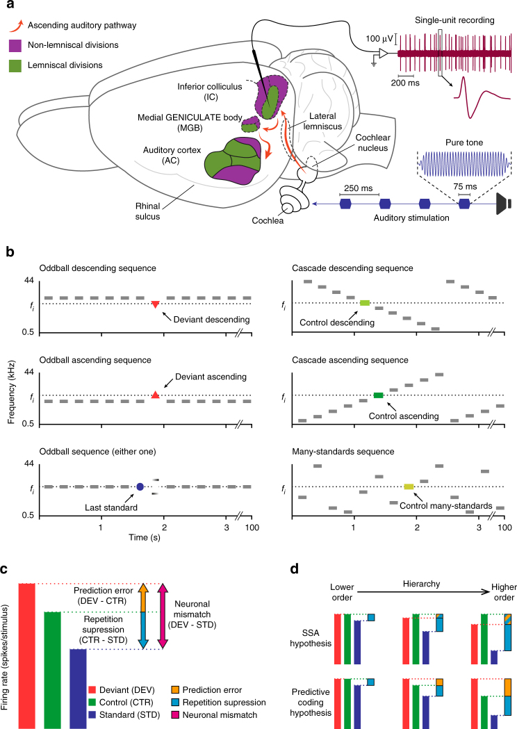
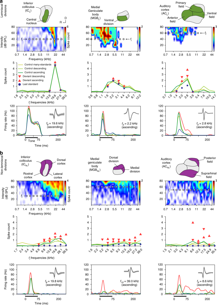
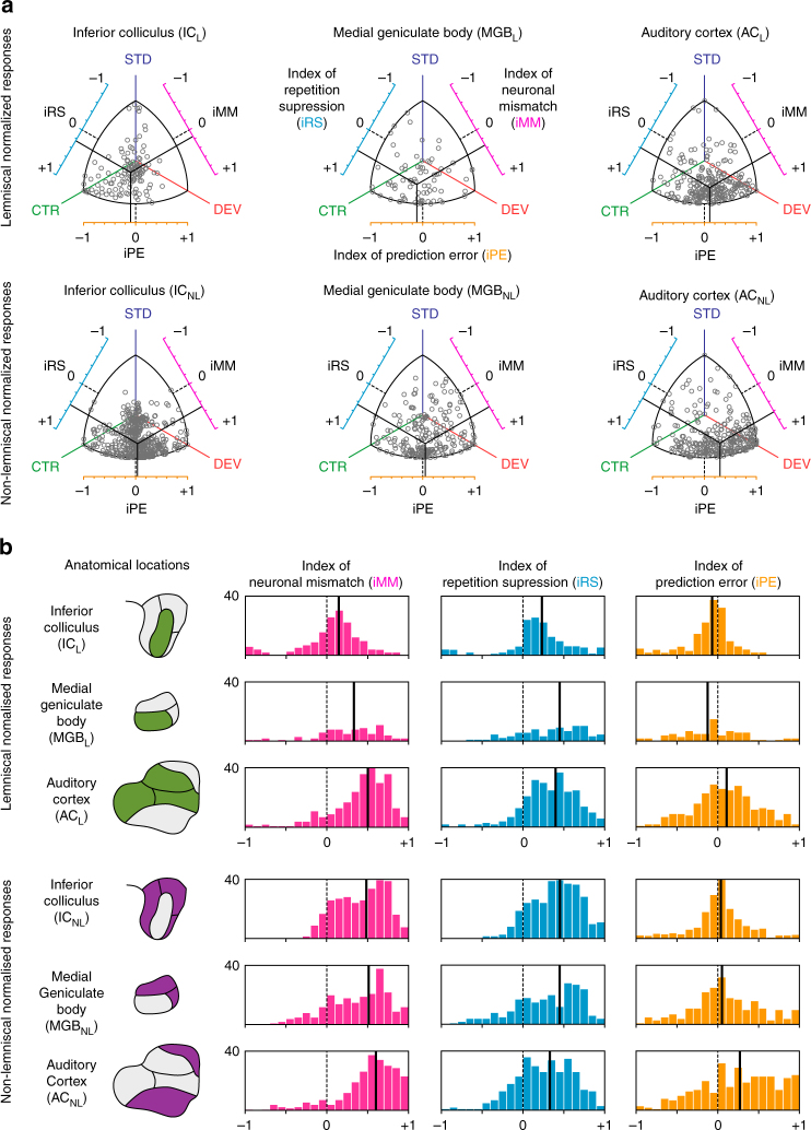
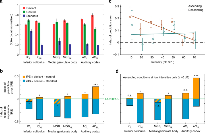
Perception is characterized by a reciprocal exchange of predictions and prediction error signals between neural regions. However, the relationship between such sensory mismatch responses and hierarchical predictive processing has not yet been demonstrated at the neuronal level in the auditory pathway. We recorded single-neuron activity from different auditory centers in anaesthetized rats and awake mice while animals were played a sequence of sounds, designed to separate the responses due to prediction error from those due to adaptation effects. Here we report that prediction error is organized hierarchically along the central auditory pathway. These prediction error signals are detectable in subcortical regions and increase as the signals move towards auditory cortex, which in turn demonstrates a large-scale mismatch potential. Finally, the predictive activity of single auditory neurons underlies automatic deviance detection at subcortical levels of processing. These results demonstrate that prediction error is a fundamental component of singly auditory neuron responses.
Overview
The claims and statistics of this paper haven’t been checked yet.
Run the check — free, no account needed. It reads the open-access text and checks the sources it cites.
Integrity signals
Registry
Cites
Statistics
Figures
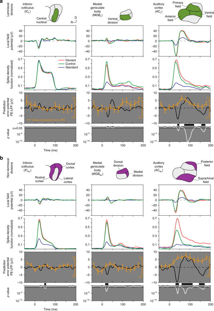
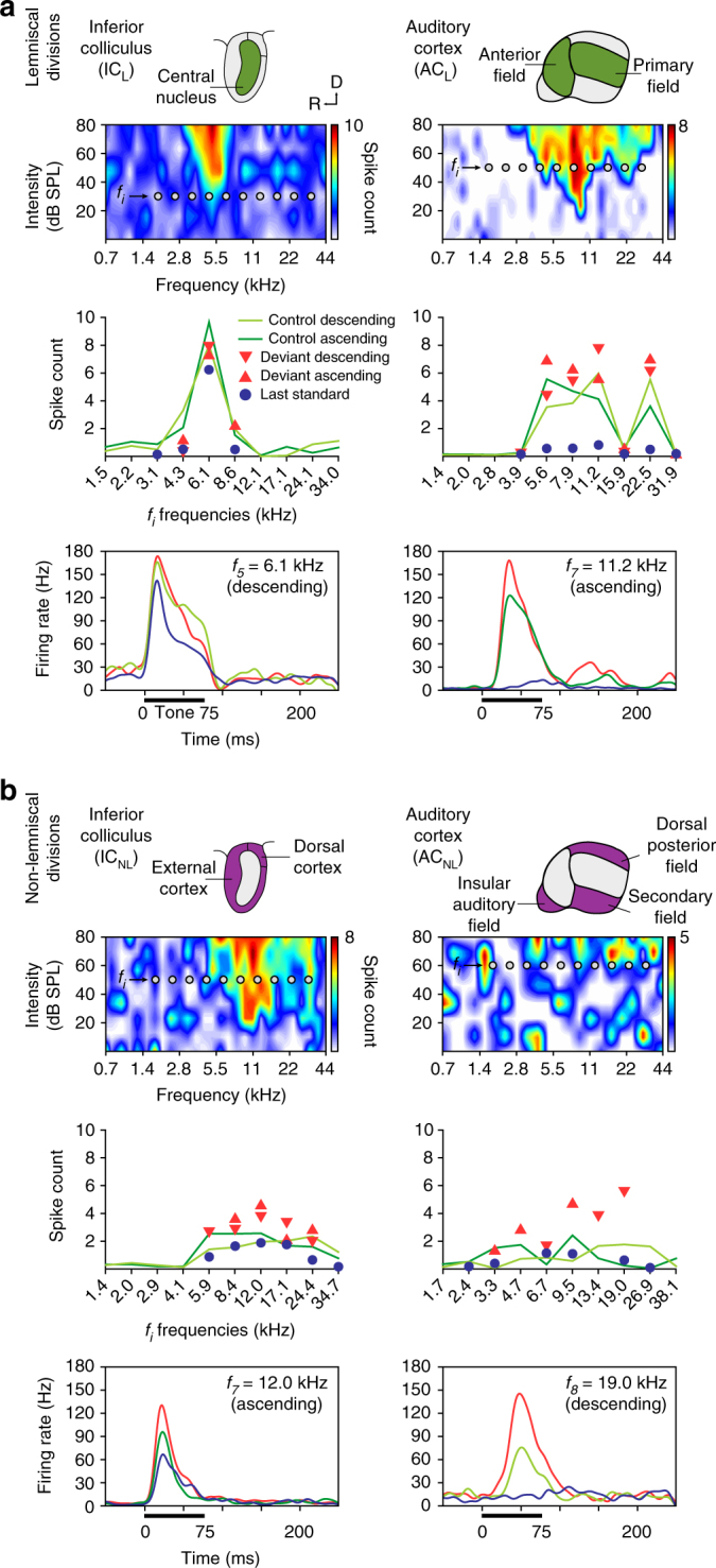
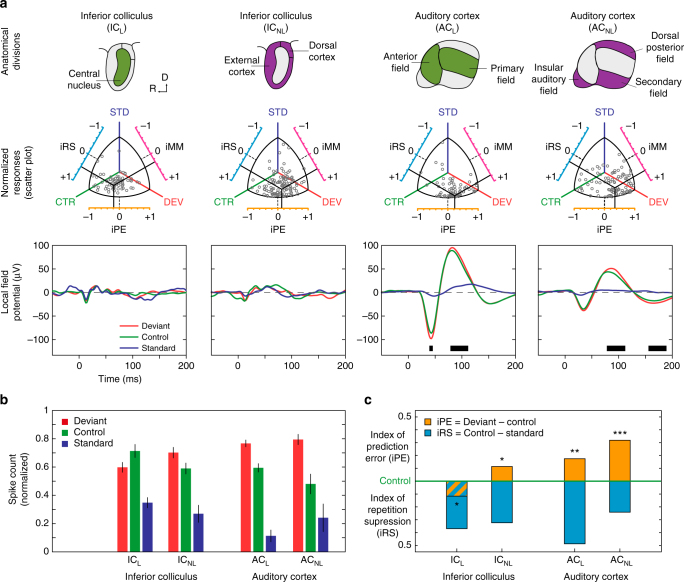
Verification
Claims the paper makes
The claims and statistics of this paper haven’t been checked yet.
Run the check — free, no account needed. It reads the open-access text and checks the sources it cites.
Claims other papers make about this one
Each is checked against this paper’s own text: does it say what the citing paper says it does?
The cited source says what the claim attributes to it.
In the citing paper
“Several paradigms shown in this article have been already used for investigations of MMN in non-human animals (49–51).”
From A Predictive Coding Perspective on Mismatch Negativity Impairment in Schizophrenia (2020) · cites this paper as [51]
Self-check
Percentages, sums and reported differences re-computed from the paper’s own numbers.
The self-check needs the paper’s full text.
Citations
Cites
The Rat Brain in Stereotaxic Coordinates
Paxinos, G., & Watson, C. (1983) · Elsevier eBooks · doi:10.1016/c2009-0-63235-9 · Cited by 28,585
The Mouse Brain in Stereotaxic Coordinates
Paxinos, G. (2001) · Cited by 12,859
Paxinos, G. (1985) · Cited by 3,715
The mismatch negativity (MMN) in basic research of central auditory processing: A review
Näätänen, R., Paavilainen, P., Rinne, T., & Alho, K. (2007) · Clinical Neurophysiology · doi:10.1016/j.clinph.2007.04.026 · Cited by 2,644
Canonical Microcircuits for Predictive Coding
Bastos, A. M., Usrey, W. M., Adams, R. A., Mangun, G. R., Fries, P., & Friston, K. J. (2012) · Neuron · doi:10.1016/j.neuron.2012.10.038 · Cited by 2,421
The free-energy principle: a rough guide to the brain?
Friston, K. (2009) · Trends in Cognitive Sciences · doi:10.1016/j.tics.2009.04.005 · Cited by 1,831
Synaptic depression and cortical gain control
Abbott, L. F., Varela, J. A., Sen, K., & Nelson, S. B. (1997) · Science · doi:10.1126/science.275.5297.221 · Cited by 1,690
The mismatch negativity: a review of underlying mechanisms
Garrido, M. I., Kilner, J. M., Stephan, K. E., & Friston, K. J. (2009) · Clinical Neurophysiology · doi:10.1016/j.clinph.2008.11.029 · Cited by 1,441
Processing of low-probability sounds by cortical neurons
Ulanovsky, N., Las, L., & Nelken, I. (2003) · Nature Neuroscience · doi:10.1038/nn1032 · Cited by 1,049
Cortical feedback improves discrimination between figure and background by V1, V2 and V3 neurons
Hupé, J. M., James, A. C., Payne, B. R., Lomber, S. G., Girard, P., & Bullier, J. (1998) · Nature · doi:10.1038/29537 · Cited by 864
Modeling the auditory scene: predictive regularity representations and perceptual objects
Winkler, I., Denham, S. L., & Nelken, I. (2009) · Trends in Cognitive Sciences · doi:10.1016/j.tics.2009.09.003 · Cited by 574
Mismatch negativity (MMN), the deviance-elicited auditory deflection, explained
May, P. J. C., & Tiitinen, H. (2010) · Psychophysiology · doi:10.1111/j.1469-8986.2009.00856.x · Cited by 549
A neuronal model of predictive coding accounting for the mismatch negativity.
Wacongne, C., Changeux, J.-P., & Dehaene, S. (2012) · The Journal of Neuroscience · doi:10.1523/jneurosci.5003-11.2012 · Cited by 542
Dehaene, S., Meyniel, F., Wacongne, C., Wang, L., & Pallier, C. (2015) · Neuron · doi:10.1016/j.neuron.2015.09.019 · Cited by 478
Great Expectations: Is there Evidence for Predictive Coding in Auditory Cortex?
Heilbron, M., & Chait, M. (2018) · Neuroscience · doi:10.1016/j.neuroscience.2017.07.061 · Cited by 428
Güntürkün, O., & Bugnyar, T. (2016) · Trends in Cognitive Sciences · doi:10.1016/j.tics.2016.02.001 · Cited by 388
Stimulus-Specific Adaptation in the Inferior Colliculus of the Anesthetized Rat
Malmierca, M. S., Cristaudo, S., Pérez‐González, D., & Covey, E. (2009) · Journal of Neuroscience · doi:10.1523/jneurosci.4153-08.2009 · Cited by 386
Self-citationEarly electrophysiological indicators for predictive processing in audition: A review
Bendixen, A., SanMiguel, I., & Schröger, E. (2011) · International Journal of Psychophysiology · doi:10.1016/j.ijpsycho.2011.08.003 · Cited by 361
Visual mismatch negativity: a predictive coding view
Stefanics, G., Kremláček, J., & Czigler, I. (2014) · Frontiers in Human Neuroscience · doi:10.3389/fnhum.2014.00666 · Cited by 360
Multiparametric Auditory Receptive Field Organization Across Five Cortical Fields in the Albino Rat
Polley, D. B., Read, H. L., Storace, D. A., & Merzenich, M. M. (2007) · Journal of Neurophysiology · doi:10.1152/jn.01298.2006 · Cited by 340
Repetition suppression and its contextual determinants in predictive coding
Auksztulewicz, R., & Friston, K. (2016) · Cortex · doi:10.1016/j.cortex.2015.11.024 · Cited by 307
The evolution of reproductive isolation through sexual conflict
Martin, O. Y., & Hosken, D. J. (2003) · Nature · doi:10.1038/nature01752 · Cited by 291
Corticocentric myopia: old bias in new cognitive sciences
Parvizi, J. (2009) · Trends in Cognitive Sciences · doi:10.1016/j.tics.2009.04.008 · Cited by 260
Umbricht, D., Koller, R., Vollenweider, F. X., & Schmid, L. (2002) · Biological Psychiatry · doi:10.1016/s0006-3223(01)01242-2 · Cited by 258
Stimulus-Specific Adaptation and Deviance Detection in the Rat Auditory Cortex
Taaseh, N., Yaron, A., & Nelken, I. (2011) · PLoS ONE · doi:10.1371/journal.pone.0023369 · Cited by 254
Disruption of hierarchical predictive coding during sleep
Strauss, M., Sitt, J. D., King, J.-R., Elbaz, M., Azizi, L., Buiatti, M., Naccache, L., van Wassenhove, V., & Dehaene, S. (2015) · Proceedings of the National Academy of Sciences · doi:10.1073/pnas.1501026112 · Cited by 244
Beaudrot, L. H., Ahumada, J., O’Brien, T. G., Álvarez-Loayza, P., Boekee, K., Campos‐Arceiz, A., Eichberg, D., Espinosa, S., Fegraus, E., Fletcher, C. D., et al. (2016) · PLoS Biology · doi:10.1371/journal.pbio.1002357 · Cited by 235
Repetition effects to sounds: evidence for predictive coding in the auditory system
Baldeweg, T. (2006) · Trends in Cognitive Sciences · doi:10.1016/j.tics.2006.01.010 · Cited by 233
Guo, W., Chambers, A. R., Darrow, K. N., Hancock, K. E., Shinn‐Cunningham, B. G., & Polley, D. B. (2012) · Journal of Neuroscience · doi:10.1523/jneurosci.0065-12.2012 · Cited by 226
Farley, B. J., Quirk, M. C., Doherty, J. J., & Christian, E. P. (2010) · The Journal of Neuroscience · doi:10.1523/jneurosci.2793-10.2010 · Cited by 183
Fishman, Y. I., & Steinschneider, M. (2012) · The Journal of Neuroscience · doi:10.1523/jneurosci.2835-12.2012 · Cited by 174
Graybiel, A. M. (1973) · Brain Research · doi:10.1016/0006-8993(73)90420-4 · Cited by 174
Unraveling the principles of auditory cortical processing: can we learn from the visual system?
King, A. J., & Nelken, I. (2009) · Nature Neuroscience · doi:10.1038/nn.2308 · Cited by 167
Somatostatin Interneurons Control a Key Component of Mismatch Negativity in Mouse Visual Cortex
Hamm, J. P., & Yuste, R. (2016) · Cell Reports · doi:10.1016/j.celrep.2016.06.037 · Cited by 165
Malmierca, M. S., Anderson, L. A., & Antunes, F. M. (2015) · Frontiers in Systems Neuroscience · doi:10.3389/fnsys.2015.00019 · Cited by 162
Self-citationHierarchy of prediction errors for auditory events in human temporal and frontal cortex
Dürschmid, S., Edwards, E., Reichert, C., Dewar, C., Hinrichs, H., Heinze, H.-J., Kirsch, H. E., Dalal, S. S., Deouell, L. Y., & Knight, R. T. (2016) · Proceedings of the National Academy of Sciences · doi:10.1073/pnas.1525030113 · Cited by 161
Bastos, A. M., Litvak, V., Moran, R., Bosman, C. A., Fries, P., & Friston, K. J. (2015) · NeuroImage · doi:10.1016/j.neuroimage.2014.12.081 · Cited by 152
Chen, I.-W., Helmchen, F., & Lütcke, H. (2015) · Journal of Neuroscience · doi:10.1523/jneurosci.2240-15.2015 · Cited by 146
Rapid Sensory Adaptation Redux: A Circuit Perspective
Whitmire, C. J., & Stanley, G. B. (2016) · Neuron · doi:10.1016/j.neuron.2016.09.046 · Cited by 145
Chemically Defined Parallel Pathways in the Monkey Auditory System
Jones, E. G. (2003) · Annals of the New York Academy of Sciences · doi:10.1196/annals.1284.033 · Cited by 141
Joan, A. L., Aitana, S., Romero, S., Miquel, M., & Jordi Riba, A. (2015) · Frontiers in Systems Neuroscience · doi:10.3389/conf.fnsys.2015.06.00008 · Cited by 141
The auditory novelty system: An attempt to integrate human and animal research
Escera, C., & Malmierca, M. S. (2013) · Psychophysiology · doi:10.1111/psyp.12156 · Cited by 139
Self-citationJavier, N.-D., & Malmierca, M. S. (2016) · PLoS Biology · doi:10.1371/journal.pbio.1002397 · Cited by 134
Self-citationThe Mechanisms and Meaning of the Mismatch Negativity
Fishman, Y. I. (2013) · Brain Topography · doi:10.1007/s10548-013-0337-3 · Cited by 127
Neuronal adaptation, novelty detection and regularity encoding in audition
Malmierca, M. S. (2014) · Frontiers in Systems Neuroscience · doi:10.3389/fnsys.2014.00111 · Cited by 116
Self-citationSensory and cognitive mechanisms for preattentive change detection in auditory cortex
Opitz, B., Schröger, E., & von Cramon, D. Y. (2005) · European Journal of Neuroscience · doi:10.1111/j.1460-9568.2005.03839.x · Cited by 116
Finding the right control: The mismatch negativity under investigation
Ruhnau, P., Herrmann, B., & Schröger, E. (2011) · Clinical Neurophysiology · doi:10.1016/j.clinph.2011.07.035 · Cited by 116
Stimulus-specific adaptation and deviance detection in the inferior colliculus
Ayala, Y. A., & Malmierca, M. S. (2013) · Frontiers in Neural Circuits · doi:10.3389/fncir.2012.00089 · Cited by 113
Self-citationDuque, D., Pérez‐González, D., Ayala, Y. A., Palmer, A. R., & Malmierca, M. S. (2012) · Journal of Neuroscience · doi:10.1523/jneurosci.3190-12.2012 · Cited by 111
Self-citationMartin, C., Houitte, D., Guillermier, M., Petit, F., Bonvento, G., & Gurden, H. (2012) · Frontiers in Neural Circuits · doi:10.3389/fncir.2012.00001 · Cited by 106
Mismatch Negativity (MMN) in Freely-Moving Rats with Several Experimental Controls
Harms, L. R., Fulham, W. R., Todd, J., Budd, T. W., Hunter, M., Meehan, C. L., Penttonen, M., Schall, U., Zavitsanou, K., Hodgson, D. M., et al. (2014) · PLoS ONE · doi:10.1371/journal.pone.0110892 · Cited by 106
Frequency discrimination and stimulus deviance in the inferior colliculus and cochlear nucleus
Ayala, Y. A., Pérez‐González, D., Duque, D., Nelken, I., & Malmierca, M. S. (2013) · Frontiers in Neural Circuits · doi:10.3389/fncir.2012.00119 · Cited by 95
Self-citationCerebral responses to local and global auditory novelty under general anesthesia
Uhrig, L., Janssen, D., Dehaene, S., & Jarraya, B. (2016) · NeuroImage · doi:10.1016/j.neuroimage.2016.08.004 · Cited by 87
On the classification of pathways in the auditory midbrain, thalamus, and cortex
Lee, C. C., & Sherman, S. M. (2010) · Hearing Research · doi:10.1016/j.heares.2010.12.012 · Cited by 80
Duque, D., & Malmierca, M. S. (2014) · Brain Structure and Function · doi:10.1007/s00429-014-0862-1 · Cited by 77
Self-citationPhillips, H. N., Blenkmann, A. O., Hughes, L. E., Kochen, S. S., Bekinschtein, T. A., Cam‐CAN, & Rowe, J. B. (2016) · Cortex · doi:10.1016/j.cortex.2016.05.001 · Cited by 77
Criteria for determining whether mismatch responses exist in animal models: Focus on rodents
Harms, L. R., Michie, P. T., & Näätänen, R. (2015) · Biological Psychology · doi:10.1016/j.biopsycho.2015.07.006 · Cited by 76
Cascaded Effects of Spatial Adaptation in the Early Visual System
Dhruv, N. T., & Carandini, M. (2014) · Neuron · doi:10.1016/j.neuron.2013.11.025 · Cited by 76
Cortical Mapping of Mismatch Negativity with Deviance Detection Property in Rat
Shiramatsu, T. I., Kanzaki, R., & Takahashi, H. (2013) · PLoS ONE · doi:10.1371/journal.pone.0082663 · Cited by 75
Peter, V., McArthur, G. M., & Thompson, W. F. (2010) · Neuroscience Letters · doi:10.1016/j.neulet.2010.07.010 · Cited by 75
Duque, D., Malmierca, M. S., & Caspary, D. M. (2013) · The Journal of Physiology · doi:10.1113/jphysiol.2013.261941 · Cited by 75
Self-citationJoachimsthaler, B., Uhlmann, M., Miller, F., Ehret, G., & Kurt, S. (2014) · European Journal of Neuroscience · doi:10.1111/ejn.12478 · Cited by 69
Cholinergic Modulation of Stimulus-Specific Adaptation in the Inferior Colliculus
Ayala, Y. A., & Malmierca, M. S. (2015) · Journal of Neuroscience · doi:10.1523/jneurosci.0909-15.2015 · Cited by 65
Self-citationVinken, K., Vogels, R., & de Beeck, H. O. (2017) · Current Biology · doi:10.1016/j.cub.2017.02.024 · Cited by 58
Ayala, Y. A., Pérez‐González, D., & Malmierca, M. S. (2015) · Biological Psychology · doi:10.1016/j.biopsycho.2015.06.016 · Cited by 56
Self-citationAn Overview of Stimulus-Specific Adaptation in the Auditory Thalamus
Antunes, F. M., & Malmierca, M. S. (2013) · Brain Topography · doi:10.1007/s10548-013-0342-6 · Cited by 56
Self-citationDuque, D., Wang, X., Javier, N.-D., Krumbholz, K., & Malmierca, M. S. (2016) · Scientific Reports · doi:10.1038/srep24114 · Cited by 56
Self-citationDeviant Processing in the Primary Somatosensory Cortex
Musall, S., Haiss, F., Weber, B., & von der Behrens, W. (2015) · Cerebral Cortex · doi:10.1093/cercor/bhv283 · Cited by 52
Ayala, Y. A., Udeh, A., Dutta, K., Bishop, D. C., Malmierca, M. S., & Oliver, D. L. (2015) · Scientific Reports · doi:10.1038/srep10383 · Cited by 51
Self-citationMittag, M., Takegata, R., & Winkler, I. (2016) · Journal of Neuroscience · doi:10.1523/jneurosci.1041-16.2016 · Cited by 40
Recasens, M., Grimm, S., Wollbrink, A., Pantev, C., & Escera, C. (2014) · Human Brain Mapping · doi:10.1002/hbm.22582 · Cited by 33
Self-citationAdaptation of high-gamma responses in human auditory association cortex
Eliades, S. J., Crone, N. E., Anderson, W. S., Ramadoss, D., Lenz, F. A., & Boatman‐Reich, D. (2014) · Journal of Neurophysiology · doi:10.1152/jn.00207.2014 · Cited by 33
Klein, C., von der Behrens, W., & Gaese, B. H. (2014) · Brain Topography · doi:10.1007/s10548-014-0376-4 · Cited by 23
Deviance detection by a P3-like response in rat posterior parietal cortex
Imada, A., Morris, A., & Wiest, M. (2013) · Frontiers in Integrative Neuroscience · doi:10.3389/fnint.2012.00127 · Cited by 22
Ayala, Y. A., Pérez‐González, D., Duque, D., Palmer, A. R., & Malmierca, M. S. (2016) · Journal of Visualized Experiments · doi:10.3791/53914 · Cited by 14
Self-citation
Cited by
Sorted by citations
How Do Expectations Shape Perception?
de Lange, F. P., Heilbron, M., & Kok, P. (2018) · Trends in Cognitive Sciences · doi:10.1016/j.tics.2018.06.002 · Cited by 975
Carbajal, G. V., & Malmierca, M. S. (2018) · Trends in Hearing · doi:10.1177/2331216518784822 · Cited by 241
Self-citationEvolving perspectives on the sources of the frequency-following response
Coffey, E. B. J., Nicol, T., White-Schwoch, T., Chandrasekaran, B., Krizman, J., Skoe, E., Zatorre, R. J., & Kraus, N. (2019) · Nature Communications · doi:10.1038/s41467-019-13003-w · Cited by 207
Making Sense of Mismatch Negativity
Fitzgerald, K. S., & Todd, J. (2020) · Frontiers in Psychiatry · doi:10.3389/fpsyt.2020.00468 · Cited by 233
Principles of large-scale neural interactions
Vinck, M. A., Uran, C., Spyropoulos, G., Onorato, I., Broggini, A. C., Schneider, M., & Canales‐Johnson, A. (2023) · Neuron · doi:10.1016/j.neuron.2023.03.015 · Cited by 170
Metadata
- Authors
- Parras, G. G., Nieto-Diego, J., Carbajal, G. V., Valdés-Baizabal, C., Escera, C., & Malmierca, M. S.
- Affiliations
- Instituto de Investigación Biomédica de Salamanca (ES)
- Institut de Recerca Sant Joan de Déu (ES)
- Universidad de Salamanca (ES)
- Corresponding author
- Malmierca, Manuel S.
- Venue
- Nature Communications
- Published
- 2017-12-15
- Volume
- 8
- Issue
- 1
- Pages
- 2148-2148
- ISSN
- 2041-1723 (ISSN-L)
- PMC
- PMC5732270
- OpenAlex
- W2774201964
- Cited by
- 344
- References
- 75
- Citations by year
- 2026: 38 · 2025: 33 · 2024: 55 · 2023: 60 · 2022: 39 · 2021: 29 · 2020: 50 · 2019: 25 · 2018: 14
- FWCI
- 13.96
- Type
- journal article
- Language
- en
- Open access
- gold
- doi.org
- Locations
- Nature Communications (publishedVersion, cc-by)
- PubMed Central (publishedVersion, cc-by)
- PubMed (publishedVersion)
- Gredos (University of Salamanca) (publishedVersion, cc-by)
- Hispana (publishedVersion, cc-by)
- RePEc: Research Papers in Economics (submittedVersion)
- Dipòsit Digital de la Universitat de Barcelona (Universitat de Barcelona) (submittedVersion, cc-by)
- DOAJ (DOAJ: Directory of Open Access Journals) (submittedVersion)
- DOAJ (DOAJ: Directory of Open Access Journals) (submittedVersion, cc-by-sa)
- Funders
- Generalitat de Catalunya (SGR 2014, SGR2014-177)
- Junta de Castilla y León
- European Social Fund (2007–2013)
- Topics
- Life Sciences › Neuroscience › Cognitive Neuroscience › Neuroscience and Music Perception
- Life Sciences › Neuroscience › Sensory Systems › Hearing, Cochlea, Tinnitus, Genetics
- Life Sciences › Neuroscience › Cognitive Neuroscience › Embodied and Extended Cognition
- Keywords
- prediction error, auditory pathway, single-unit activity, auditory cortex, subcortical auditory processing, mismatch response, deviance detection, sensory prediction, auditory adaptation
About these checks
Registry, retraction, Cites and statistics results are computed, not judged, with one exception: a printed reference that no index lists is read once by a model before it counts as a citation error. Claims are extracted by a model and kept only when their quote appears verbatim in the text; each cited source is then checked, with a model’s help, for whether it says what the claim relies on. Those verdicts can be wrong — read the claim’s quote and the cited source before relying on one.
Statistics and arithmetic are recomputed, not judged.
Confidence bands are shown only for fields calibrated on our annotated test set. None is calibrated yet, so no band is shown.
What counts as a claim ›How we measure confidence ›How we check this ›
Are you an author, or do you see a problem with this page? Request a review
