

The DOI matches its Crossref record; 94 of the 94 references it cites were found in a registry or an index.
Metastable brain waves
Open accessPublished version of a preprint
Abstract
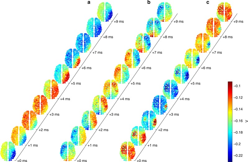
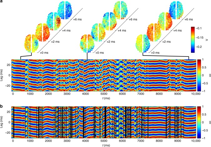
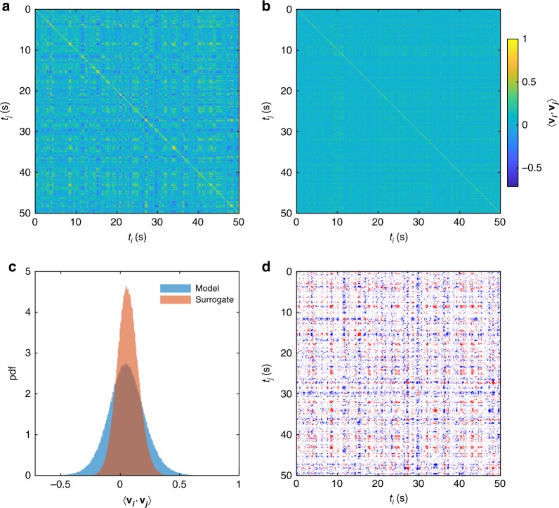
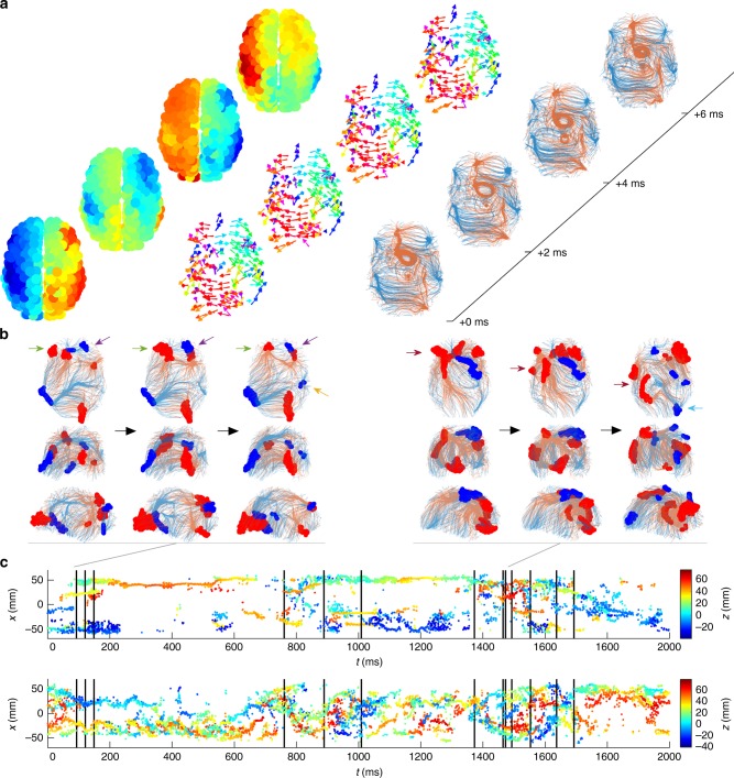
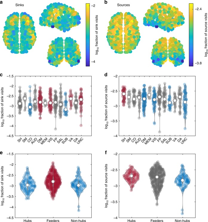
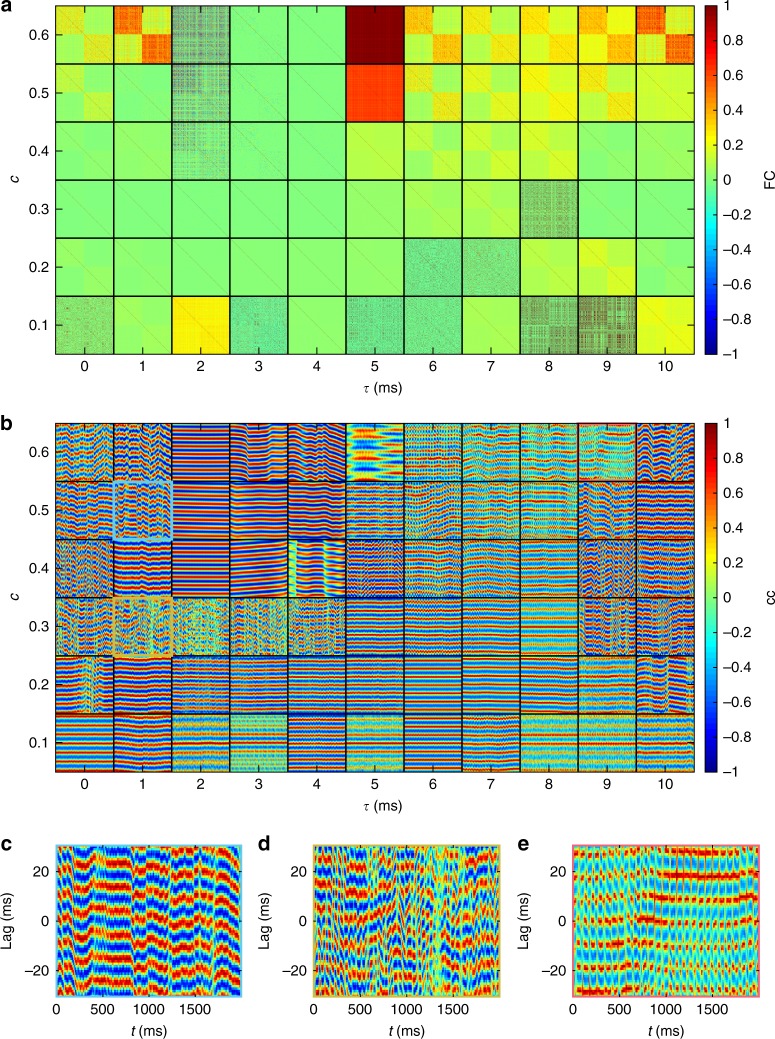
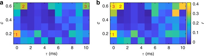
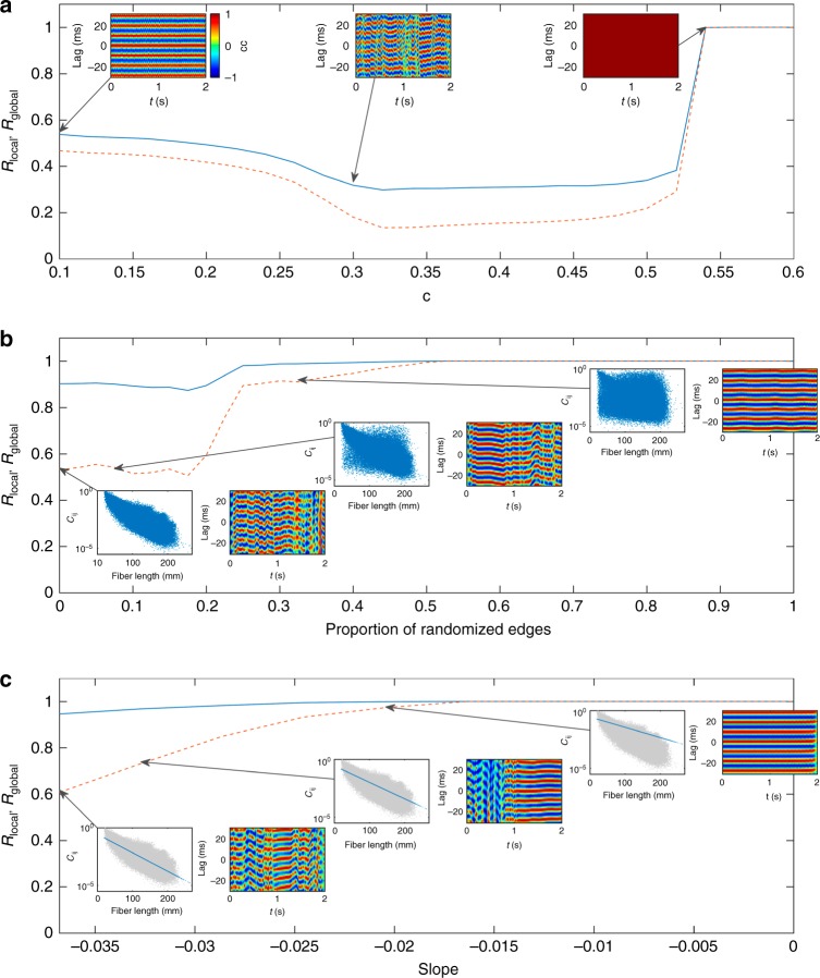
Traveling patterns of neuronal activity—brain waves—have been observed across a breadth of neuronal recordings, states of awareness, and species, but their emergence in the human brain lacks a firm understanding. Here we analyze the complex nonlinear dynamics that emerge from modeling large-scale spontaneous neural activity on a whole-brain network derived from human tractography. We find a rich array of three-dimensional wave patterns, including traveling waves, spiral waves, sources, and sinks. These patterns are metastable, such that multiple spatiotemporal wave patterns are visited in sequence. Transitions between states correspond to reconfigurations of underlying phase flows, characterized by nonlinear instabilities. These metastable dynamics accord with empirical data from multiple imaging modalities, including electrical waves in cortical tissue, sequential spatiotemporal patterns in resting-state MEG data, and large-scale waves in human electrocorticography. By moving the study of functional networks from a spatially static to an inherently dynamic (wave-like) frame, our work unifies apparently diverse phenomena across functional neuroimaging modalities and makes specific predictions for further experimentation.
Overview
The claims and statistics of this paper haven’t been checked yet.
Run the check — free, no account needed. It reads the open-access text and checks the sources it cites.
Integrity signals
Registry
Cites
Statistics
Figures
Verification
Claims the paper makes
The claims and statistics of this paper haven’t been checked yet.
Run the check — free, no account needed. It reads the open-access text and checks the sources it cites.
Claims other papers make about this one
Each is checked against this paper’s own text: does it say what the citing paper says it does?
The check wasn’t confident either way, so it gives no verdict — never disputed.
In the citing paper
“Evidence suggests that neural fluctuations involve multiplicative rather than merely additive noise components, where the variance of the noise depends on the system’s state (Buice et al. 2010; Roberts et al. 2019).”
From The myth of the Bayesian brain (2025) · cites this paper as Roberts et al. 2019
Experimental — accuracy not yet measured
Self-check
Percentages, sums and reported differences re-computed from the paper’s own numbers.
The self-check needs the paper’s full text.
Citations
Cites
Complex network measures of brain connectivity: Uses and interpretations
Rubinov, M., & Sporns, O. (2010) · NeuroImage · doi:10.1016/j.neuroimage.2009.10.003 · Cited by 11,522
Mapping the structural core of human cerebral cortex
Hagmann, P., Cammoun, L., Gigandet, X., Meuli, R., Honey, C. J., Wedeen, V. J., & Sporns, O. (2008) · PLoS Biology · doi:10.1371/journal.pbio.0060159 · Cited by 4,173
Functional Network Organization of the Human Brain
Power, J. D., Cohen, A. L., Nelson, S. M., Wig, G. S., Barnes, K. A., Church, J. A., Vogel, A. C., Laumann, T. O., Miezin, F. M., Schlaggar, B. L., et al. (2011) · Neuron · doi:10.1016/j.neuron.2011.09.006 · Cited by 4,124
Excitatory and Inhibitory Interactions in Localized Populations of Model Neurons
Wilson, H. R., & Cowan, J. D. (1972) · Biophysical Journal · doi:10.1016/s0006-3495(72)86068-5 · Cited by 3,579
Predicting human resting-state functional connectivity from structural connectivity
Honey, C. J., Sporns, O., Cammoun, L., Gigandet, X., Thiran, J. P., Meuli, R., & Hagmann, P. (2009) · Proceedings of the National Academy of Sciences · doi:10.1073/pnas.0811168106 · Cited by 3,307
Rhythms for cognition: communication through coherence
Fries, P. (2015) · Neuron · doi:10.1016/j.neuron.2015.09.034 · Cited by 2,725
Tournier, J., Calamante, F., & Connelly, A. (2007) · NeuroImage · doi:10.1016/j.neuroimage.2007.02.016 · Cited by 2,191
Network structure of cerebral cortex shapes functional connectivity on multiple time scales
Honey, C. J., Kötter, R., Breakspear, M. J., & Sporns, O. (2007) · Proceedings of the National Academy of Sciences · doi:10.1073/pnas.0701519104 · Cited by 1,727
Self-citationMRtrix: Diffusion tractography in crossing fiber regions
Tournier, J., Calamante, F., & Connelly, A. (2012) · International Journal of Imaging Systems and Technology · doi:10.1002/ima.22005 · Cited by 1,370
Dynamic models of large-scale brain activity
Breakspear, M. (2017) · Nature Neuroscience · doi:10.1038/nn.4497 · Cited by 1,239
Self-citationWhole-brain anatomical networks: does the choice of nodes matter?
Zalesky, A., Fornito, A., Harding, I. H., Cocchi, L., Yücel, M., Pantelis, C., & Bullmore, E. T. (2010) · NeuroImage · doi:10.1016/j.neuroimage.2009.12.027 · Cited by 1,169
Nonlinear Responses in fMRI: The Balloon Model, Volterra Kernels, and Other Hemodynamics
Friston, K. J., Mechelli, A., Turner, R., & Price, C. J. (2000) · NeuroImage · doi:10.1006/nimg.2000.0630 · Cited by 1,131
Stochastic resonance without tuning
Collins, J. J., Chow, C. C., & Imhoff, T. T. (1995) · Nature · doi:10.1038/376236a0 · Cited by 821
High-cost, high-capacity backbone for global brain communication
van den Heuvel, M. P., Kahn, R. S., Goñi, J., & Sporns, O. (2012) · Proceedings of the National Academy of Sciences · doi:10.1073/pnas.1203593109 · Cited by 781
Key role of coupling, delay, and noise in resting brain fluctuations
Deco, G., Jirsa, V., McIntosh, A. R., Sporns, O., & Kötter, R. (2009) · Proceedings of the National Academy of Sciences · doi:10.1073/pnas.0901831106 · Cited by 777
On the nature of seizure dynamics
Jirsa, V., Stacey, W. C., Quilichini, P., Ivanov, A., & Bernard, C. (2014) · Brain · doi:10.1093/brain/awu133 · Cited by 760
Time-resolved resting-state brain networks
Zalesky, A., Fornito, A., Cocchi, L., Gollo, L. L., & Breakspear, M. (2014) · Proceedings of the National Academy of Sciences · doi:10.1073/pnas.1400181111 · Cited by 753
Ongoing Cortical Activity at Rest: Criticality, Multistability, and Ghost Attractors
Deco, G., & Jirsa, V. (2012) · Journal of Neuroscience · doi:10.1523/jneurosci.2523-11.2012 · Cited by 704
Cortical travelling waves: mechanisms and computational principles
Muller, L., Chavane, F., Reynolds, J. H., & B, T. J. S. A. (2018) · Nature reviews. Neuroscience · doi:10.1038/nrn.2018.20 · Cited by 617
A mathematical theory of visual hallucination patterns
Ermentrout, B., & Cowan, J. D. (1979) · Biological Cybernetics · doi:10.1007/bf00336965 · Cited by 594
Deco, G., Ponce-Alvarez, A., Mantini, D., Romani, G. L., Hagmann, P., & Corbetta, M. (2013) · Journal of Neuroscience · doi:10.1523/jneurosci.1091-13.2013 · Cited by 576
Fast transient networks in spontaneous human brain activity
Baker, A. P., Brookes, M. J., Rezek, I. A., Smith, S. M., Behrens, T. E. J., Probert-Smith, P., & Woolrich, M. W. (2014) · eLife · doi:10.7554/elife.01867 · Cited by 569
Self-citationCriticality in the brain: A synthesis of neurobiology, models and cognition
Cocchi, L., Gollo, L. L., Zalesky, A., & Breakspear, M. J. (2017) · Progress in Neurobiology · doi:10.1016/j.pneurobio.2017.07.002 · Cited by 555
Self-citationRole of local network oscillations in resting-state functional connectivity
Cabral, J., Hugues, E., Sporns, O., & Deco, G. (2011) · NeuroImage · doi:10.1016/j.neuroimage.2011.04.010 · Cited by 531
Generative Models of Cortical Oscillations: Neurobiological Implications of the Kuramoto Model
Breakspear, M. J., Heitmann, S., & Daffertshofer, A. (2010) · Frontiers in Human Neuroscience · doi:10.3389/fnhum.2010.00190 · Cited by 531
Self-citationOn the stability of BOLD fMRI correlations
Laumann, T. O., Snyder, A. Z., Mitra, A., Gordon, E. M., Gratton, C., Adeyemo, B., Gilmore, A. W., Nelson, S. M., Berg, J. J., Greene, D. J., et al. (2016) · Cerebral Cortex · doi:10.1093/cercor/bhw265 · Cited by 516
Propagating waves mediate information transfer in the motor cortex
Rubino, D., Robbins, K. A., & Hatsopoulos, N. G. (2006) · Nature Neuroscience · doi:10.1038/nn1802 · Cited by 508
Propagation and stability of waves of electrical activity in the cerebral cortex
Robinson, P. A., RENNIE, C. J., & Wright, J. J. (1997) · Physical review. E, Statistical physics, plasmas, fluids, and related interdisciplinary topics · doi:10.1103/physreve.56.826 · Cited by 486
Breakspear, M. J., Roberts, J. A., Terry, J. R., Rodrigues, S., Mahant, N., & Robinson, P. A. (2005) · Cerebral Cortex · doi:10.1093/cercor/bhj072 · Cited by 463
Self-citationWaves, bumps, and patterns in neural field theories
Coombes, S. (2005) · Biological Cybernetics · doi:10.1007/s00422-005-0574-y · Cited by 450
Deco, G., & Kringelbach, M. L. (2014) · Neuron · doi:10.1016/j.neuron.2014.08.034 · Cited by 416
Spatiotemporal dynamics of continuum neural fields
Bressloff, P. C. (2011) · Journal of Physics A Mathematical and Theoretical · doi:10.1088/1751-8113/45/3/033001 · Cited by 412
Spiral Waves in Disinhibited Mammalian Neocortex
Huang, X., Troy, W. C., Yang, Q., Ma, H., Laing, C. R., Schiff, S. J., & Wu, J. (2004) · Journal of Neuroscience · doi:10.1523/jneurosci.2705-04.2004 · Cited by 388
Spontaneous cortical activity transiently organises into frequency specific phase-coupling networks
Vidaurre, D., Hunt, L. T., Quinn, A. J., Hunt, B. A. E., Brookes, M. J., Nobre, A. C., & Woolrich, M. W. (2018) · Nature Communications · doi:10.1038/s41467-018-05316-z · Cited by 384
Self-citationHuman brain networks function in connectome-specific harmonic waves
Atasoy, S., Donnelly, I., & Pearson, J. (2016) · Nature Communications · doi:10.1038/ncomms10340 · Cited by 381 · cited 1×
“The linear treatment of cortical waves under idealized assumptions regarding cortico-cortical connectivity has been well-studied [33, 34], particularly for standing waves [35, 36], as has neuronal wave pattern formation in abstract mathematical settings [26, 37-41].”
BackgroundSpontaneous cortical activity alternates between motifs defined by regional axonal projections
Mohajerani, M. H., Chan, A. W., Mohsenvand, M. ‘., LeDue, J. M., Liu, R., McVea, D. A., Boyd, J. D., Wang, Y. T., Reimers, M., & Murphy, T. H. (2013) · Nature Neuroscience · doi:10.1038/nn.3499 · Cited by 375
Transient Cognitive Dynamics, Metastability, and Decision Making
Rabinovich, M. I., Huerta, R., Varona, P., & Afraimovich, V. (2008) · PLoS Computational Biology · doi:10.1371/journal.pcbi.1000072 · Cited by 364
The dynamics of chimera states in heterogeneous Kuramoto networks
Laing, C. R. (2009) · Physica D Nonlinear Phenomena · doi:10.1016/j.physd.2009.04.012 · Cited by 325
Visual stimuli induce waves of electrical activity in turtle cortex
Prechtl, J. C., Cohen, L. B., Pesaran, B., Mitra, P. P., & Kleinfeld, D. (1997) · Proceedings of the National Academy of Sciences · doi:10.1073/pnas.94.14.7621 · Cited by 321
Cabral, J., Luckhoo, H., Woolrich, M. W., Joensson, M., Mohseni, H., Baker, A. P., Kringelbach, M. L., & Deco, G. (2013) · NeuroImage · doi:10.1016/j.neuroimage.2013.11.047 · Cited by 320
Self-citationSalami, M., Itami, C., Tsumoto, T., & Kimura, F. (2003) · Proceedings of the National Academy of Sciences · doi:10.1073/pnas.0937380100 · Cited by 314
Traveling Waves in Visual Cortex
Sato, T. K., Nauhaus, I., & Carandini, M. (2012) · Neuron · doi:10.1016/j.neuron.2012.06.029 · Cited by 288
Dynamics of travelling waves in visual perception
Wilson, H. R., Blake, R., & Lee, S.-H. (2001) · Nature · doi:10.1038/35091066 · Cited by 287
Nunez, P. L., & Srinivasan, R. (2006) · Clinical Neurophysiology · doi:10.1016/j.clinph.2006.06.754 · Cited by 281
Reverberation of recent visual experience in spontaneous cortical waves
Han, F., Caporale, N., & Dan, Y. (2008) · Neuron · doi:10.1016/j.neuron.2008.08.026 · Cited by 268
Interpreting temporal fluctuations in resting-state functional connectivity MRI
Liégeois, R., Laumann, T. O., Snyder, A. Z., Zhou, J. H., & Yeo, B. T. T. (2017) · NeuroImage · doi:10.1016/j.neuroimage.2017.09.012 · Cited by 264
The stimulus-evoked population response in visual cortex of awake monkey is a propagating wave
Muller, L., Reynaud, A., Chavane, F., & Alain Destexhe, A. (2014) · Nature Communications · doi:10.1038/ncomms4675 · Cited by 259
Traveling waves of activity in primary visual cortex during binocular rivalry
Lee, S., Blake, R., & Heeger, D. J. (2004) · Nature Neuroscience · doi:10.1038/nn1365 · Cited by 258
Mohajerani, M. H., McVea, D. A., Fingas, M., & Murphy, T. H. (2010) · Journal of Neuroscience · doi:10.1523/jneurosci.6437-09.2010 · Cited by 256
Standing waves and traveling waves distinguish two circuits in visual cortex
Benucci, A., Frazor, R. A., & Carandini, M. (2007) · Neuron · doi:10.1016/j.neuron.2007.06.017 · Cited by 254
Propagating Waves of Activity in the Neocortex: What They Are, What They Do
Wu, J., Huang, X., & Zhang, C. (2007) · The Neuroscientist · doi:10.1177/1073858408317066 · Cited by 253
Caminiti, R., Carducci, F., Piervincenzi, C., Battaglia‐Mayer, A., Confalone, G., Visco‐Comandini, F., Pantano, P., & Innocenti, G. M. (2013) · Journal of Neuroscience · doi:10.1523/jneurosci.0761-13.2013 · Cited by 221
Kaneko, K., & Tsuda, I. (2003) · Chaos An Interdisciplinary Journal of Nonlinear Science · doi:10.1063/1.1607783 · Cited by 221
Muller, L., Piantoni, G., Koller, D. P., Cash, S. S., Halgren, E., & B, T. J. S. A. (2016) · eLife · doi:10.7554/elife.17267 · Cited by 215
The contribution of geometry to the human connectome
Roberts, J. A., Perry, A., Lord, A. R., Roberts, G., Mitchell, P. B., Smith, R. E., Calamante, F., & Breakspear, M. (2016) · NeuroImage · doi:10.1016/j.neuroimage.2015.09.009 · Cited by 213
Self-citationDeco, G., Cabral, J., Woolrich, M. W., Stevner, A. B. A., van Hartevelt, T. J., & Kringelbach, M. L. (2017) · NeuroImage · doi:10.1016/j.neuroimage.2017.03.023 · Cited by 193
Self-citationDwelling quietly in the rich club: brain network determinants of slow cortical fluctuations
Gollo, L. L., Zalesky, A., Hutchison, R. M., van den Heuvel, M. P., & Breakspear, M. J. (2015) · Philosophical Transactions of the Royal Society B Biological Sciences · doi:10.1098/rstb.2014.0165 · Cited by 189
Self-citationConsistency-based thresholding of the human connectome
Roberts, J. A., Perry, A., Roberts, G., Mitchell, P. B., & Breakspear, M. (2017) · NeuroImage · doi:10.1016/j.neuroimage.2016.09.053 · Cited by 189
Self-citationA Canonical Model of Multistability and Scale-Invariance in Biological Systems
Freyer, F., Roberts, J. A., Ritter, P., & Breakspear, M. J. (2012) · PLoS Computational Biology · doi:10.1371/journal.pcbi.1002634 · Cited by 186
Self-citationBreakspear, M. J., Terry, J. R., & Friston, K. J. (2003) · Network Computation in Neural Systems · doi:10.1088/0954-898x/14/4/305 · Cited by 176
Self-citationSteady-state visual evoked potentials and travelling waves
Burkitt, G., Silberstein, R. B., Cadusch, P. J., & Wood, A. (2000) · Clinical Neurophysiology · doi:10.1016/s1388-2457(99)00194-7 · Cited by 172
Roberts, G. M. P., Lord, A., Frankland, A., Wright, A., Lau, P., Lévy, F., Lenroot, R., Mitchell, P. B., & Breakspear, M. J. (2016) · Biological Psychiatry · doi:10.1016/j.biopsych.2016.08.018 · Cited by 157
Self-citationThe ictal wavefront is the spatiotemporal source of discharges during spontaneous human seizures
Smith, E. H., Liou, J.-Y., Davis, T. S., Merricks, E. M., Kellis, S., Weiss, S. A., Greger, B. E., House, P. A., McKhann, G. M., Goodman, R. R., et al. (2016) · Nature Communications · doi:10.1038/ncomms11098 · Cited by 156
Mapping how local perturbations influence systems-level brain dynamics
Gollo, L. L., Roberts, J. A., & Cocchi, L. (2017) · NeuroImage · doi:10.1016/j.neuroimage.2017.01.057 · Cited by 144
Self-citationA Sensorimotor Role for Traveling Waves in Primate Visual Cortex
Zanos, T. P., Mineault, P., Nasiotis, K., Guitton, D., & Pack, C. C. (2015) · Neuron · doi:10.1016/j.neuron.2014.12.043 · Cited by 139
Eigenmodes of brain activity: Neural field theory predictions and comparison with experiment
Robinson, P. A., Zhao, X., Aquino, K. M., Griffiths, J. D., Sarkar, S., & Mehta-Pandejee, G. (2016) · NeuroImage · doi:10.1016/j.neuroimage.2016.04.050 · Cited by 129
Human seizures couple across spatial scales through travelling wave dynamics
Martinet, L.-E., Fiddyment, G. M., Madsen, J. R., Eskandar, E. N., Truccolo, W., Eden, U. T., Cash, S. S., & Kramer, M. (2017) · Nature Communications · doi:10.1038/ncomms14896 · Cited by 127
Besserve, M., Lowe, S., Logothetis, N. K., Schölkopf, B., & Panzeri, S. (2015) · PLoS Biology · doi:10.1371/journal.pbio.1002257 · Cited by 116
Propagating waves in thalamus, cortex and the thalamocortical system: Experiments and models
Muller, L., & Alain Destexhe, A. (2012) · Journal of Physiology-Paris · doi:10.1016/j.jphysparis.2012.06.005 · Cited by 108
Breakspear, M. J., Terry, J. R., & Friston, K. J. (2003) · Network Computation in Neural Systems · doi:10.1088/0954-898x_14_4_305 · Cited by 107
Self-citationWill a Large Complex System with Time Delays Be Stable?
Jirsa, V., & Ding, M. (2004) · Physical Review Letters · doi:10.1103/physrevlett.93.070602 · Cited by 106
Messé, A., Rudrauf, D., Giron, A., & Marrelec, G. (2015) · NeuroImage · doi:10.1016/j.neuroimage.2015.02.001 · Cited by 106
Fragility and volatility of structural hubs in the human connectome
Gollo, L. L., Roberts, J. A., Cropley, V., Biase, M. A. D., Pantelis, C., Zalesky, A., & Breakspear, M. J. (2018) · Nature Neuroscience · doi:10.1038/s41593-018-0188-z · Cited by 105
Self-citationAbeysuriya, R., Hadida, J., Sotiropoulos, S. N., Jbabdi, S., Becker, R., Hunt, B. A. E., Brookes, M. J., & Woolrich, M. W. (2018) · PLoS Computational Biology · doi:10.1371/journal.pcbi.1006007 · Cited by 96
Self-citationPerturbation of whole-brain dynamics in silico reveals mechanistic differences between brain states
Deco, G., Cabral, J., Saenger, V. M., Boly, M., Tagliazucchi, E., Laufs, H., Someren, E. J. W. V., Jobst, B., Stevner, A. B. A., & Kringelbach, M. L. (2017) · NeuroImage · doi:10.1016/j.neuroimage.2017.12.009 · Cited by 94
The frustrated brain: from dynamics on motifs to communities and networks
Gollo, L. L., & Breakspear, M. J. (2014) · Philosophical Transactions of the Royal Society B Biological Sciences · doi:10.1098/rstb.2013.0532 · Cited by 90
Self-citationBressloff, P. C. (2013) · Lecture notes on mathematical modelling in the life sciences · doi:10.1007/978-1-4614-8866-8 · Cited by 87
Hemodynamic Traveling Waves in Human Visual Cortex
Aquino, K. M., Schira, M. M., Robinson, P. A., Drysdale, P. M., & Breakspear, M. J. (2012) · PLoS Computational Biology · doi:10.1371/journal.pcbi.1002435 · Cited by 86
Self-citationRobinson, P. A. (2012) · Physical Review E · doi:10.1103/physreve.85.011912 · Cited by 83
Intra-cortical propagation of EEG alpha oscillations
Hindriks, R., van Putten, M. J. A. M., & Deco, G. (2014) · NeuroImage · doi:10.1016/j.neuroimage.2014.08.027 · Cited by 82
Emergence of Complex Wave Patterns in Primate Cerebral Cortex
Townsend, R. G., Solomon, S. S., Chen, S. C., Pietersen, A. N. J., Martin, P. R., Solomon, S. G., & Gong, P. (2015) · Journal of Neuroscience · doi:10.1523/jneurosci.4509-14.2015 · Cited by 80
Lu, Y., Truccolo, W., Wagner, F. B., Vargas-Irwin, C. E., Ozden, I., Zimmermann, J. B., May, T., Agha, N. S., Wang, J., & Nurmikko, A. V. (2015) · Journal of Neurophysiology · doi:10.1152/jn.00792.2014 · Cited by 69
The organisation of the elderly connectome
Perry, A., Wen, W. X., Lord, A., Thalamuthu, A., Roberts, G. M. P., Mitchell, P. B., Sachdev, P. S., & Breakspear, M. J. (2015) · NeuroImage · doi:10.1016/j.neuroimage.2015.04.009 · Cited by 60
Self-citationUsing computational models to relate structural and functional brain connectivity
Hlinka, J., & Coombes, S. (2012) · European Journal of Neuroscience · doi:10.1111/j.1460-9568.2012.08081.x · Cited by 58
Large-Scale Cortical Dynamics of Sleep Slow Waves
Botella‐Soler, V., Valderrama, M., Crépon, B., Navarro, V., & Quyen, M. L. V. (2012) · PLoS ONE · doi:10.1371/journal.pone.0030757 · Cited by 42
Deconvolution of neural dynamics from fMRI data using a spatiotemporal hemodynamic response function
Aquino, K. M., Robinson, P. A., Schira, M. M., & Breakspear, M. J. (2014) · NeuroImage · doi:10.1016/j.neuroimage.2014.03.001 · Cited by 42
Self-citationClinical Applications of Stochastic Dynamic Models of the Brain, Part I: A Primer
Roberts, J. A., Friston, K. J., & Breakspear, M. J. (2017) · Biological Psychiatry Cognitive Neuroscience and Neuroimaging · doi:10.1016/j.bpsc.2017.01.010 · Cited by 41
Self-citationModeling distributed axonal delays in mean-field brain dynamics
Roberts, J. A., & Robinson, P. A. (2008) · Physical Review E · doi:10.1103/physreve.78.051901 · Cited by 39
Self-citationA Dendritic Mechanism for Decoding Traveling Waves: Principles and Applications to Motor Cortex
Heitmann, S., Boonstra, T. W., & Breakspear, M. J. (2013) · PLoS Computational Biology · doi:10.1371/journal.pcbi.1003260 · Cited by 33
Self-citationIlloul, L., & Lorong, P. (2011) · Computers & Structures · doi:10.1016/j.compstruc.2011.01.018 · Cited by 31
Visual Motion Discrimination by Propagating Patterns in Primate Cerebral Cortex
Townsend, R. G., Solomon, S. S., Martin, P. R., Solomon, S. G., & Gong, P. (2017) · Journal of Neuroscience · doi:10.1523/jneurosci.1538-17.2017 · Cited by 28
Global Neuromagnetic Cortical Fields Have Non-Zero Velocity
Alexander, D. M., Nikolaev, A. R., Jurica, P., Zvyagintsev, M., Mathiak, K., & van Leeuwen, C. (2016) · PLoS ONE · doi:10.1371/journal.pone.0148413 · Cited by 27
Heitmann, S., Rule, M. E., Truccolo, W., & Ermentrout, B. (2017) · PLoS Computational Biology · doi:10.1371/journal.pcbi.1005349 · Cited by 21
Waves in Spatially-Disordered Neural Fields: A Case Study in Uncertainty Quantification
Laing, C. R. (2015) · Studies in mechanobiology, tissue engineering and biomaterials · doi:10.1007/978-3-319-21296-8_14 · Cited by 5
Research works printed but not linked: 1
- Ester, M., Kriegel, H. -P., Sander, J. & Xu, X. in Proc. Second International Conference on Knowledge Discovery and Data Mining 226–231 (AAAI Press).
Cited by
Sorted by citations
Linking Structure and Function in Macroscale Brain Networks
Suárez, L. E., Markello, R. D., Betzel, R. F., & Mišić, B. (2020) · Trends in Cognitive Sciences · doi:10.1016/j.tics.2020.01.008 · Cited by 769
Questions and controversies in the study of time-varying functional connectivity in resting fMRI
Lurie, D. J., Kessler, D., Bassett, D. S., Betzel, R. F., Breakspear, M., Kheilholz, S., Kucyi, A., Liégeois, R., Lindquist, M. A., McIntosh, A. R., et al. (2020) · Network Neuroscience · doi:10.1162/netn_a_00116 · Cited by 648
Self-citationGeometric constraints on human brain function
Pang, J. C. S., Aquino, K. M., Oldehinkel, M., Robinson, P. A., Fulcher, B., Breakspear, M. J., & Fornito, A. (2023) · Nature · doi:10.1038/s41586-023-06098-1 · Cited by 470
Self-citationDecoupling of brain function from structure reveals regional behavioral specialization in humans
Preti, M. G., & Ville, D. V. D. (2019) · Nature Communications · doi:10.1038/s41467-019-12765-7 · Cited by 337
Temporal circuit of macroscale dynamic brain activity supports human consciousness
Huang, Z., Zhang, J., Wu, J., Mashour, G. A., & Hudetz, A. G. (2020) · Science Advances · doi:10.1126/sciadv.aaz0087 · Cited by 217
Metadata
- Authors
- Roberts, J. A., Gollo, L. L., Abeysuriya, R. G., Roberts, G., Mitchell, P. B., Woolrich, M. W., & Breakspear, M.
- Affiliations
- QIMR Berghofer Medical Research Institute (AU)
- University of Oxford (GB)
- Black Dog Institute (AU)
- Corresponding author
- Roberts, James A.
- ORCID
- Venue
- Nature Communications
- Published
- 2019-03-05
- Volume
- 10
- Issue
- 1
- Pages
- 1056-1056
- ISSN
- 2041-1723 (ISSN-L)
- PMC
- PMC6401142
- OpenAlex
- W2950869179
- Cited by
- 264
- References
- 94
- Citations by year
- 2026: 32 · 2025: 42 · 2024: 36 · 2023: 41 · 2022: 37 · 2021: 26 · 2020: 30 · 2019: 19
- FWCI
- 16.27
- Type
- journal article
- Language
- en
- Open access
- gold
- doi.org
- Locations
- Nature Communications (publishedVersion, cc-by)
- bioRxiv (Cold Spring Harbor Laboratory) (acceptedVersion, cc-by-nc-nd)
- Europe PMC (PubMed Central) (publishedVersion, cc-by)
- PubMed Central (publishedVersion, cc-by)
- PubMed (publishedVersion)
- RePEc: Research Papers in Economics (submittedVersion)
- DOAJ (DOAJ: Directory of Open Access Journals) (submittedVersion)
- DOAJ (DOAJ: Directory of Open Access Journals) (submittedVersion, cc-by-sa)
- Figshare (submittedVersion, cc-by)
- NOVA (University of Newcastle Australia) (submittedVersion, cc-by)
- Funders
- Wellcome Trust (MR/K005464/1, 106183/Z/14/Z, 203139/Z/16/Z, 106183, 203139, 203139/Z/16)
- University of Nottingham
- Medical Research Council (203139/Z/16/Z, MR/K005464/1)
- Australian Research Council (1118153, 1144936, CE140100007)
- National Health and Medical Research Council (1145168, CE140100007, 1144936, 1110975, 1118153, 1037196)
- Centre of Excellence for Integrative Brain Function, Australian Research Council (CE140100007)
- Topics
- Life Sciences › Neuroscience › Cognitive Neuroscience › Neural dynamics and brain function
- Life Sciences › Neuroscience › Cognitive Neuroscience › Functional Brain Connectivity Studies
- Physical Sciences › Physics and Astronomy › Statistical and Nonlinear Physics › Nonlinear Dynamics and Pattern Formation
- Keywords
- neural oscillations, traveling waves, spiral waves, metastable dynamics, nonlinear dynamics, whole-brain networks, phase flow, nonlinear instability, spontaneous neuronal activity, resting-state MEG, electrocorticography, functional networks
- MeSH terms
- Electrocorticography, Adolescent, Adult, Brain, Computer Simulation, Female, Humans, Male, Models, Neurological, Nerve Net, Neurons, Nonlinear Dynamics, Young Adult, Diffusion Tensor Imaging, Brain Waves, Healthy Volunteers
About these checks
Registry, retraction, Cites and statistics results are computed, not judged, with one exception: a printed reference that no index lists is read once by a model before it counts as a citation error. Claims are extracted by a model and kept only when their quote appears verbatim in the text; each cited source is then checked, with a model’s help, for whether it says what the claim relies on. Those verdicts can be wrong — read the claim’s quote and the cited source before relying on one.
Statistics and arithmetic are recomputed, not judged.
Confidence bands are shown only for fields calibrated on our annotated test set. None is calibrated yet, so no band is shown.
What counts as a claim ›How we measure confidence ›How we check this ›
Are you an author, or do you see a problem with this page? Request a review
