

The DOI matches its Crossref record; 56 of the 56 references it cites were found in a registry or an index.
Clustering of single-cell multi-omics data with a multimodal deep learning method
Open accessAbstract
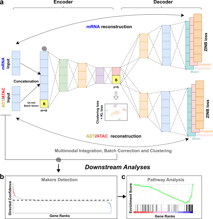
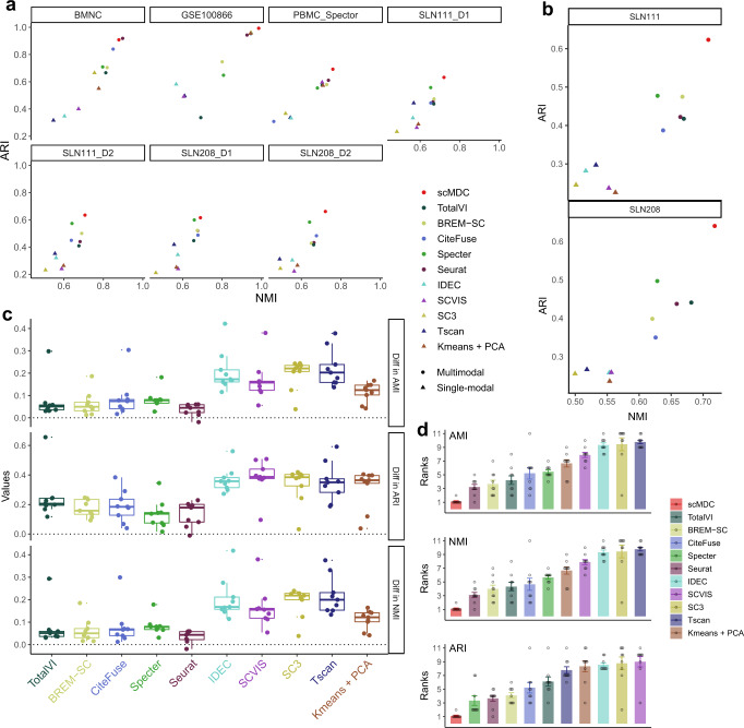
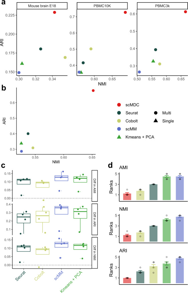
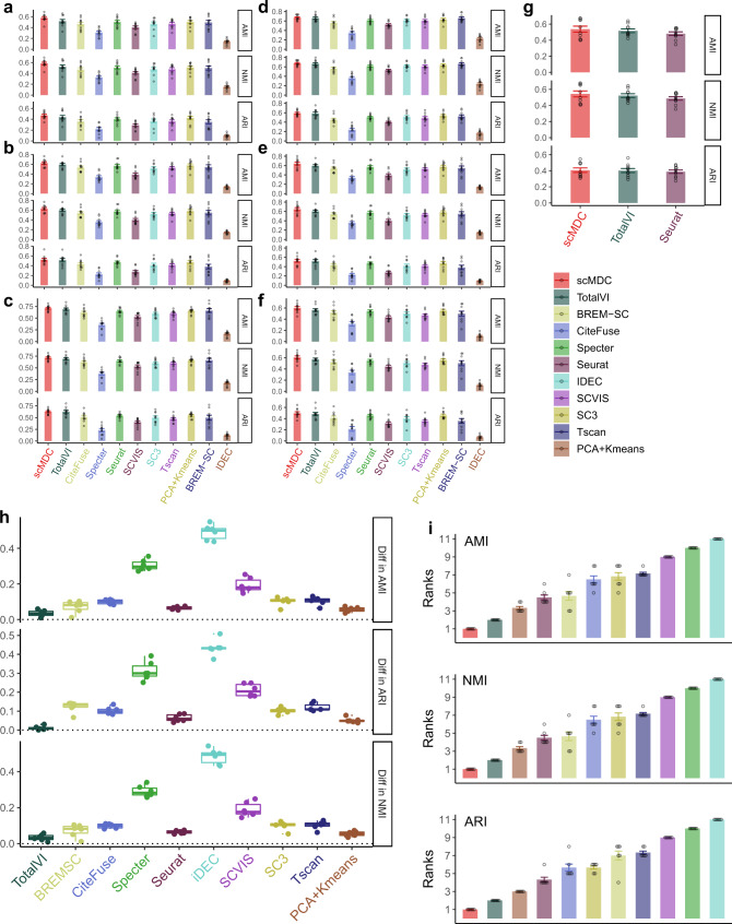
Single-cell multimodal sequencing technologies are developed to simultaneously profile different modalities of data in the same cell. It provides a unique opportunity to jointly analyze multimodal data at the single-cell level for the identification of distinct cell types. A correct clustering result is essential for the downstream complex biological functional studies. However, combining different data sources for clustering analysis of single-cell multimodal data remains a statistical and computational challenge. Here, we develop a novel multimodal deep learning method, scMDC, for single-cell multi-omics data clustering analysis. scMDC is an end-to-end deep model that explicitly characterizes different data sources and jointly learns latent features of deep embedding for clustering analysis. Extensive simulation and real-data experiments reveal that scMDC outperforms existing single-cell single-modal and multimodal clustering methods on different single-cell multimodal datasets. The linear scalability of running time makes scMDC a promising method for analyzing large multimodal datasets.
Overview
The claims and statistics of this paper haven’t been checked yet.
Run the check — free, no account needed. It reads the open-access text and checks the sources it cites.
Integrity signals
Registry
Cites
Statistics
Figures
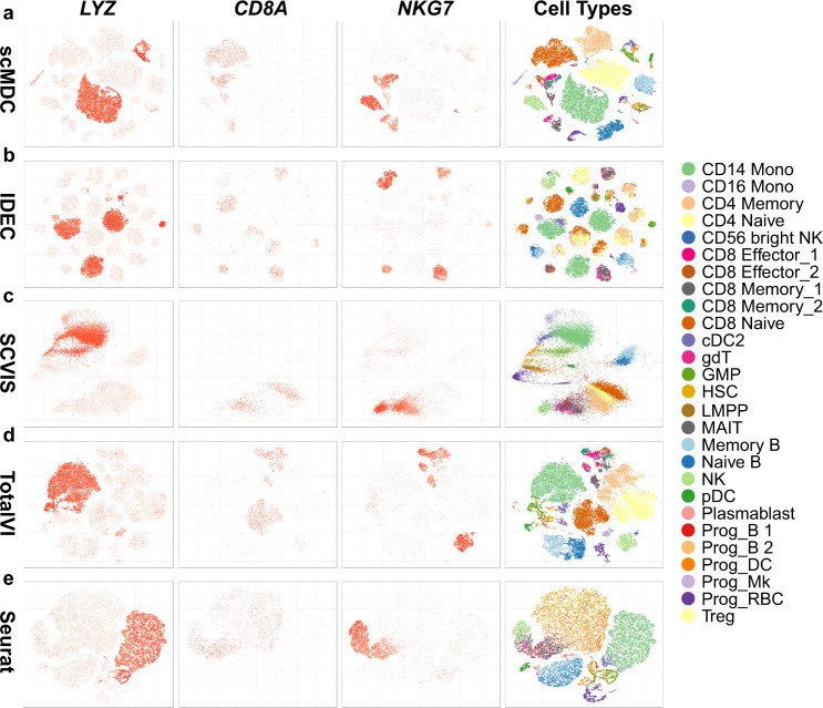
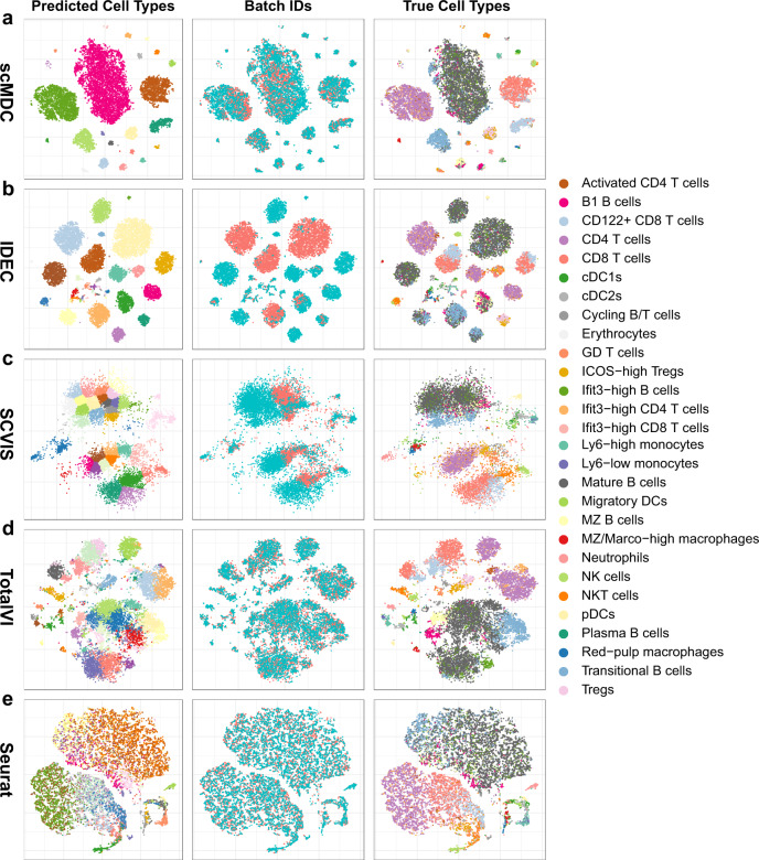
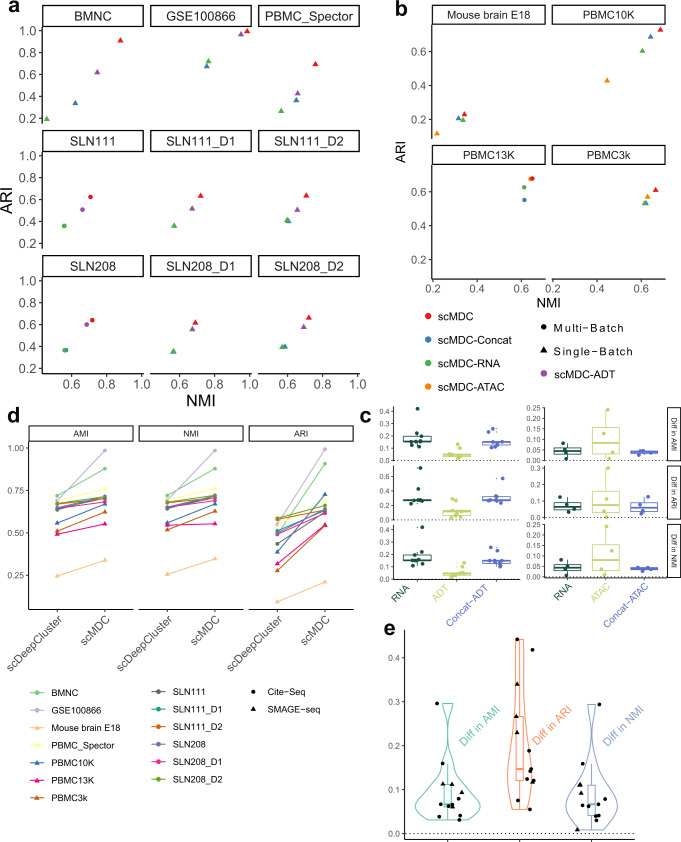
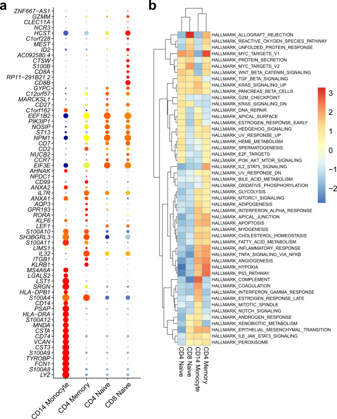
Verification
Claims the paper makes
The claims and statistics of this paper haven’t been checked yet.
Run the check — free, no account needed. It reads the open-access text and checks the sources it cites.
Claims other papers make about this one
Each is checked against this paper’s own text: does it say what the citing paper says it does?
The cited source says what the claim attributes to it.
In the citing paper
“For integrating multi-omics datasets from paired or unpaired single cells, Lin et al. introduced the scMDC method, which utilized an end-to-end autoencoder model to learn the joint embeddings of paired single-cell multi-omics datasets [119].”
From Challenges in AI-driven Biomedical Multimodal Data Fusion and Analysis (2025) · cites this paper as [119]
Self-check
Percentages, sums and reported differences re-computed from the paper’s own numbers.
The self-check needs the paper’s full text.
Citations
Cites
Moderated estimation of fold change and dispersion for RNA-seq data with DESeq2
Love, M. I., Huber, W., & Anders, S. (2014) · Genome Biology · doi:10.1186/s13059-014-0550-8 · Cited by 95,106
Fast unfolding of communities in large networks
Blondel, V. D., Guillaume, J.-L., Lambiotte, R., & Lefebvre, E. (2008) · Journal of Statistical Mechanics: Theory and Experiment · doi:10.1088/1742-5468/2008/10/p10008 · Cited by 21,424
Reducing the dimensionality of data with neural networks
Hinton, G. E., & Salakhutdinov, R. R. (2006) · Science · doi:10.1126/science.1127647 · Cited by 20,928
Integrated analysis of multimodal single-cell data
Hao, Y., Hao, S., Andersen-Nissen, E., Mauck, W. M., Zheng, S., Butler, A., Lee, M. J., Wilk, A. J., Darby, C., Zagar, M., et al. (2020) · doi:10.1101/2020.10.12.335331 · Cited by 15,508
Integrating single-cell transcriptomic data across different conditions, technologies, and species
Butler, A., Hoffman, P., Smibert, P., Papalexi, E., & Satija, R. (2018) · Nature Biotechnology · doi:10.1038/nbt.4096 · Cited by 13,174
(2017) · Cited by 11,625
SCANPY: large-scale single-cell gene expression data analysis
Wolf, F. A., Angerer, P., & Theis, F. J. (2018) · Genome Biology · doi:10.1186/s13059-017-1382-0 · Cited by 8,881
Double-slit photoelectron interference in strong-field ionization of the neon dimer
Kunitski, M., Eicke, N., Huber, P., Köhler, J., Zeller, S., Voigtsberger, J., Schlott, N., Henrichs, K., Sann, H., Trinter, F., et al. (2019) · Institutional Repository of Leibniz Universität Hannover (Leibniz Universität Hannover) · doi:10.15488/5174 · Cited by 8,378
Hubert, L., & Arabie, P. (1985) · Journal of Classification · doi:10.1007/bf01908075 · Cited by 8,219
Double-slit photoelectron interference in strong-field ionization of the neon dimer
Kunitski, M., Eicke, N., Huber, P., Köhler, J., Zeller, S., Voigtsberger, J., Schlott, N., Henrichs, K., Sann, H., Trinter, F., et al. (2019) · Nature Communications · doi:10.1038/s41467-018-07882-8 · Cited by 8,162
Extracting and composing robust features with denoising autoencoders
Vincent, P., Larochelle, H., Bengio, Y., & Manzagol, P.-A. (2008) · Proceedings of the 25th international conference on Machine learning - ICML '08 · doi:10.1145/1390156.1390294 · Cited by 7,436
Massively parallel digital transcriptional profiling of single cells
Zheng, G. X. Y., Terry, J. M., Belgrader, P., Ryvkin, P., Bent, Z. W., Wilson, R., Ziraldo, S. B., Wheeler, T. D., McDermott, G. P., Zhu, J., et al. (2017) · Nature Communications · doi:10.1038/ncomms14049 · Cited by 7,353
Cell types in the mouse cortex and hippocampus revealed by single-cell RNA-seq
Zeisel, A., Muñoz-Manchado, A. B., Codeluppi, S., Lönnerberg, P., La Manno, G., Juréus, A., Marques, S., Munguba, H., He, L., Betsholtz, C., et al. (2015) · Science · doi:10.1126/science.aaa1934 · Cited by 3,124
Simultaneous epitope and transcriptome measurement in single cells
Stoeckius, M., Hafemeister, C., Stephenson, W., Houck-Loomis, B., Chattopadhyay, P. K., Swerdlow, H., Satija, R., & Smibert, P. (2017) · Nature Methods · doi:10.1038/nmeth.4380 · Cited by 3,098
Deep generative modeling for single-cell transcriptomics
Lopez, R., Regier, J., Cole, M. B., Jordan, M. I., & Yosef, N. (2018) · Nature Methods · doi:10.1038/s41592-018-0229-2 · Cited by 2,530
Single-cell chromatin accessibility reveals principles of regulatory variation
Buenrostro, J. D., Wu, B., Litzenburger, U. M., Ruff, D., Gonzales, M. L., Snyder, M. P., Chang, H. Y., & Greenleaf, W. J. (2015) · Nature · doi:10.1038/nature14590 · Cited by 2,308
Similarity network fusion for aggregating data types on a genomic scale
Wang, B., Mezlini, A. M., Demir, F., Fiume, M., Tu, Z., Brudno, M., Haibe-Kains, B., & Goldenberg, A. (2014) · Nature Methods · doi:10.1038/nmeth.2810 · Cited by 2,036
McCarthy, D. J., Campbell, K. R., Lun, A. T. L., & Wills, Q. F. (2017) · Bioinformatics · doi:10.1093/bioinformatics/btw777 · Cited by 1,852
Harding, S. D., Sharman, J. L., Faccenda, E., Southan, C., Pawson, A. J., Ireland, S. M., Gray, A. J. G., Bruce, L., Alexander, S. P. H., Anderton, S. M., et al. (2017) · Nucleic Acids Research · doi:10.1093/nar/gkx1121 · Cited by 1,650
SC3: consensus clustering of single-cell RNA-seq data
Kiselev, V. Y., Kirschner, K., Schaub, M. T., Andrews, T., Yiu, A., Chandra, T., Natarajan, K. N., Reik, W., Barahona, M., Green, A. R., et al. (2017) · Nature Methods · doi:10.1038/nmeth.4236 · Cited by 1,500
The Technology and Biology of Single-Cell RNA Sequencing
Kolodziejczyk, A. A., Kim, J. K., Svensson, V., Marioni, J. C., & Teichmann, S. A. (2015) · Molecular Cell · doi:10.1016/j.molcel.2015.04.005 · Cited by 1,487
Multiplex single-cell profiling of chromatin accessibility by combinatorial cellular indexing
Cusanovich, D. A., Daza, R., Adey, A., Pliner, H. A., Christiansen, L., Gunderson, K. L., Steemers, F. J., Trapnell, C., & Shendure, J. (2015) · Science · doi:10.1126/science.aab1601 · Cited by 1,248
Challenges in unsupervised clustering of single-cell RNA-seq data
Kiselev, V. Y., Andrews, T. S., & Hemberg, M. (2019) · Nature Reviews Genetics · doi:10.1038/s41576-018-0088-9 · Cited by 1,184
Single-cell sequencing-based technologies will revolutionize whole-organism science
Shapiro, E., Biezuner, T., & Linnarsson, S. (2013) · Nature Reviews Genetics · doi:10.1038/nrg3542 · Cited by 1,177
Chromatin Potential Identified by Shared Single-Cell Profiling of RNA and Chromatin
Ma, S., Zhang, B., LaFave, L. M., Earl, A. S., Chiang, Z., Hu, Y., Ding, J., Brack, A., Kartha, V. K., Tay, T., et al. (2020) · Cell · doi:10.1016/j.cell.2020.09.056 · Cited by 1,146
Single-cell RNA-seq denoising using a deep count autoencoder
Eraslan, G., Simon, L. M., Mircea, M., Mueller, N. S., & Theis, F. J. (2019) · Nature Communications · doi:10.1038/s41467-018-07931-2 · Cited by 1,084
Signaling and Function of Interleukin-2 in T Lymphocytes
Ross, S. H., & Cantrell, D. A. (2018) · Annual Review of Immunology · doi:10.1146/annurev-immunol-042617-053352 · Cited by 1,015
Multiplexed quantification of proteins and transcripts in single cells
Peterson, V. M., Zhang, K. X., Kumar, N., Wong, J., Li, L., Wilson, D. C., Moore, R., McClanahan, T. K., Sadekova, S., & Klappenbach, J. A. (2017) · Nature Biotechnology · doi:10.1038/nbt.3973 · Cited by 832
High-throughput sequencing of the transcriptome and chromatin accessibility in the same cell
Chen, S., Lake, B. B., & Zhang, K. (2019) · Nature Biotechnology · doi:10.1038/s41587-019-0290-0 · Cited by 810
A general and flexible method for signal extraction from single-cell RNA-seq data
Risso, D., Perraudeau, F., Gribkova, S., Dudoit, S., & Vert, J.-P. (2018) · Nature Communications · doi:10.1038/s41467-017-02554-5 · Cited by 718
TSCAN: Pseudo-time reconstruction and evaluation in single-cell RNA-seq analysis
Ji, Z., & Ji, H. (2016) · Nucleic Acids Research · doi:10.1093/nar/gkw430 · Cited by 643
Joint probabilistic modeling of single-cell multi-omic data with totalVI
Gayoso, A., Steier, Z., Lopez, R., Regier, J., Nazor, K. L., Streets, A., & Yosef, N. (2021) · Nature Methods · doi:10.1038/s41592-020-01050-x · Cited by 592
Mimitou, E. P., Cheng, A., Montalbano, A., Hao, S., Stoeckius, M., Legut, M., Roush, T., Herrera, A., Papalexi, E., Ouyang, Z., et al. (2019) · Nature Methods · doi:10.1038/s41592-019-0392-0 · Cited by 520
Integrated Analysis of Transcriptomic and Proteomic Data
Haider, S., & Pal, R. (2013) · Current Genomics · doi:10.2174/1389202911314020003 · Cited by 446
Clustering single-cell RNA-seq data with a model-based deep learning approach
Tian, T., Wan, J., Song, Q., & Wei, Z. (2019) · Nature Machine Intelligence · doi:10.1038/s42256-019-0037-0 · Cited by 437
Self-citationInterpretable dimensionality reduction of single cell transcriptome data with deep generative models
Ding, J., Condon, A., & Shah, S. P. (2018) · Nature Communications · doi:10.1038/s41467-018-04368-5 · Cited by 337
Integrative Methods and Practical Challenges for Single-Cell Multi-omics
Ma, A., McDermaid, A., Xu, J., Chang, Y., & Ma, Q. (2020) · Trends in biotechnology · doi:10.1016/j.tibtech.2020.02.013 · Cited by 278
Marchingo, J. M., Sinclair, L. V., Howden, A. J. M., & Cantrell, D. A. (2020) · eLife · doi:10.7554/elife.53725 · Cited by 202
Cobolt: integrative analysis of multimodal single-cell sequencing data
Gong, B., Zhou, Y., & Purdom, E. (2021) · Genome Biology · doi:10.1186/s13059-021-02556-z · Cited by 168
Model-based deep embedding for constrained clustering analysis of single cell RNA-seq data
Tian, T., Zhang, J., Lin, X., Wei, Z., & Hakonarson, H. H. (2021) · Nature Communications · doi:10.1038/s41467-021-22008-3 · Cited by 150
Self-citationMultimodal single-cell chromatin analysis with SignacPreprint
Stuart, T., Srivastava, A., Lareau, C. A., & Satija, R. (2020) · bioRxiv (Cold Spring Harbor Laboratory) · doi:10.1101/2020.11.09.373613 · Cited by 150
A mixture-of-experts deep generative model for integrated analysis of single-cell multiomics data
Minoura, K., Abe, K., Nam, H., Nishikawa, H., & Shimamura, T. (2021) · Cell Reports Methods · doi:10.1016/j.crmeth.2021.100071 · Cited by 145
Variational autoencoders for cancer data integration: design principles and computational practice
Simidjievski, N., Bodnar, C., Tariq, I., Scherer, P., Andres Terre, H., Shams, Z., Jamnik, M., & Liò, P. (2019) · Frontiers in Genetics · doi:10.3389/fgene.2019.01205 · Cited by 145
Deep soft K-means clustering with self-training for single-cell RNA sequence data
Chen, L., Wang, W., Zhai, Y., & Deng, M. (2020) · NAR Genomics and Bioinformatics · doi:10.1093/nargab/lqaa039 · Cited by 145
Cho, S. H., Raybuck, A. L., Blagih, J., Kemboi, E., Haase, V. H., Jones, R. G., & Boothby, M. R. (2019) · Proceedings of the National Academy of Sciences · doi:10.1073/pnas.1811702116 · Cited by 139
Dynamic Roles for IL-2–STAT5 Signaling in Effector and Regulatory CD4+ T Cell Populations
Jones, D. M., Read, K. A., & Oestreich, K. J. (2020) · The Journal of Immunology · doi:10.4049/jimmunol.2000612 · Cited by 139
Simulating multiple faceted variability in single cell RNA sequencing
Zhang, X., Xu, C. A., & Yosef, N. (2019) · Nature Communications · doi:10.1038/s41467-019-10500-w · Cited by 121
CiteFuse enables multi-modal analysis of CITE-seq data
Kim, H. J., Lin, Y., Geddes, T. A., Yang, J. Y. H., & Yang, P. (2020) · Bioinformatics · doi:10.1093/bioinformatics/btaa282 · Cited by 103
BREM-SC: a bayesian random effects mixture model for joint clustering single cell multi-omics data
Wang, X., Sun, Z., Zhang, Y., Xu, Z., Xin, H., Huang, H., Duerr, R. H., Chen, K., Ding, Y., & Chen, W. (2020) · Nucleic Acids Research · doi:10.1093/nar/gkaa314 · Cited by 99
The Immune-Metabolic Basis of Effector Memory CD4+ T Cell Function under Hypoxic Conditions
Dimeloe, S., Mehling, M., Frick, C., Loeliger, J., Bantug, G. R., Sauder, U., Fischer, M., Belle, R., Develioglu, L., Tay, S., et al. (2015) · The Journal of Immunology · doi:10.4049/jimmunol.1501766 · Cited by 91
A monocyte gene expression signature in the early clinical course of Parkinson’s disease
Schlachetzki, J. C. M., Prots, I., Tao, J., Chun, H. B., Saijo, K., Gosselin, D., Winner, B., Glass, C. K., & Winkler, J. (2018) · Scientific Reports · doi:10.1038/s41598-018-28986-7 · Cited by 58
Atypical Human Effector/Memory CD4+ T Cells With a Naive-Like Phenotype
Caccamo, N., Joosten, S. A., Ottenhoff, T. H. M., & Dieli, F. (2018) · Frontiers in Immunology · doi:10.3389/fimmu.2018.02832 · Cited by 56
Hasan, F., Chiu, Y., Shaw, R., Wang, J., & Yee, C. (2021) · JCI Insight · doi:10.1172/jci.insight.138970 · Cited by 56
The Complement System Is Essential for the Phagocytosis of Mesenchymal Stromal Cells by Monocytes
Gavin, C., Meinke, S., Heldring, N., Heck, K. A., Achour, A., Iacobaeus, E., Höglund, P., Blanc, K. L., & Kadri, N. (2019) · Frontiers in Immunology · doi:10.3389/fimmu.2019.02249 · Cited by 53
Linear-time cluster ensembles of large-scale single-cell RNA-seq and multimodal dataPreprint
Do, V. H., Ringeling, F. R., & Canzar, S. (2021) · Genome Research · doi:10.1101/gr.267906.120 · Cited by 28
ACE: Explaining cluster from an adversarial perspectivePreprint
Lu, Y. Y., Yu, T. C., Bonora, G., & Noble, W. S. (2021) · bioRxiv (Cold Spring Harbor Laboratory) · doi:10.1101/2021.02.08.428881 · Cited by 3
Research works printed but not linked: 10
- Ng, A., Jordan, M. & Weiss, Y. On spectral clustering: analysis and an algorithm. Adv. Neural Inf. Process. Syst. 14, 849–856 (2001).
- Xie, J., Girshick, R. & Farhadi, A. Unsupervised Deep Embedding for Clustering Analysis. In: (eds Balcan, M. F. & Weinberger, K. Q.) Proceedings of Machine Learning Research Vol. 48, 478–487 (PMLR, 2016).
- Lu, Y. Y., Timothy, C. Y., Bonora, G. & Noble, W. S. ACE: Explaining cluster from an adversarial perspective. In: (eds Meila, M. & Zhang, T.) International Conference on Machine Learning. 7156–7167 (PMLR).
- Clevert, D.-A., Unterthiner, T. & Hochreiter, S. Fast and accurate deep network learning by exponential linear units (ELUs). Preprint at https://arxiv.org/abs/1511.07289 (2015). · arXiv
- Maaten, L. V. D. & Hinton, G. Visualizing data using t-SNE. J. Mach. Learn. Res. 9, 2579–2605 (2008).
- Reddi, S. J., Kale, S. & Kumar, S. On the convergence of adam and beyond. arXiv preprint arXiv:1904.09237 (2019). · arXiv
- Kingma, D. P. & Ba, J. Adam: a method for stochastic optimization. Preprint at https://arxiv.org/abs/1412.6980 (2014). · arXiv
- Zeiler, M. D. ADADELTA: an adaptive learning rate method. Preprint at https://arxiv.org/abs/1212.5701 (2012). · arXiv
- Vinh, N. X., Epps, J. & Bailey, J. Information theoretic measures for clusterings comparison: Variants, properties, normalization and correction for chance. J. Mach. Learn. Res. 11, 2837–2854 (2010).
- Alexander, S. & Joydeep, G. Cluster ensembles—a knowledge reuse framework for combining multiple partitions. J. Mach. Learn Res 3, 583–617 (2003).
Cited by
Sorted by citations
Baião, A. R., Cai, Z., Poulos, R. C., Robinson, P. J., Reddel, R. R., Zhong, Q., Vinga, S., & Gonçalves, E. (2025) · Briefings in Bioinformatics · doi:10.1093/bib/bbaf355 · Cited by 274
Multimodal deep learning approaches for single-cell multi-omics data integration
Athaya, T., Ripan, R. C., Li, X., & Hu, H. (2023) · Briefings in Bioinformatics · doi:10.1093/bib/bbad313 · Cited by 96
Yang, X., Mann, K. K., Wu, H., & Ding, J. (2024) · Genome biology · doi:10.1186/s13059-024-03338-z · Cited by 106
Mosaic integration and knowledge transfer of single-cell multimodal data with MIDAS
He, Z., Hu, S., Chen, Y., An, S., Zhou, J., Liu, R., Shi, J., Wang, J., Dong, G., Shi, J., et al. (2024) · Nature Biotechnology · doi:10.1038/s41587-023-02040-y · Cited by 84
Challenges in AI-driven Biomedical Multimodal Data Fusion and Analysis
Liu, J., Cen, X., Yi, C., Wang, F.-A., Ding, J., Cheng, J., Wu, Q., Gai, B., Zhou, Y., He, R., et al. (2025) · Genomics, Proteomics & Bioinformatics · doi:10.1093/gpbjnl/qzaf011 · Cited by 75
Metadata
- Authors
- Lin, X., Tian, T., Wei, Z., & Hakonarson, H.
- Affiliations
- New Jersey Institute of Technology (US)
- Children's Hospital of Philadelphia (US)
- Corresponding author
- Wei, Zhi
- Venue
- Nature Communications
- Published
- 2022-12-13
- Volume
- 13
- Issue
- 1
- Pages
- 7705-7705
- ISSN
- 2041-1723 (ISSN-L)
- PMC
- PMC9748135
- OpenAlex
- W4311232381
- Cited by
- 135
- References
- 56
- Citations by year
- 2026: 45 · 2025: 43 · 2024: 39 · 2023: 7 · 2022: 1
- FWCI
- 7.35
- Type
- journal article
- Language
- en
- Open access
- gold
- doi.org
- Locations
- Nature Communications (publishedVersion, cc-by)
- PubMed Central (publishedVersion, cc-by)
- PubMed (publishedVersion)
- RePEc: Research Papers in Economics (submittedVersion)
- DOAJ (DOAJ: Directory of Open Access Journals) (submittedVersion, cc-by-sa)
- Funders
- U.S. Department of Health & Human Services | NIH | National Center for Advancing Translational Sciences (UL1TR003017)
- Topics
- Life Sciences › Biochemistry, Genetics and Molecular Biology › Molecular Biology › Single-cell and spatial transcriptomics
- Life Sciences › Biochemistry, Genetics and Molecular Biology › Molecular Biology › Gene expression and cancer classification
- Life Sciences › Biochemistry, Genetics and Molecular Biology › Biophysics › Cell Image Analysis Techniques
- Keywords
- single-cell multi-omics, multimodal deep learning, cell type annotation, single-cell sequencing
- MeSH terms
- Deep Learning, Multiomics, Computer Simulation, Cluster Analysis, Single-Cell Analysis
About these checks
Registry, retraction, Cites and statistics results are computed, not judged, with one exception: a printed reference that no index lists is read once by a model before it counts as a citation error. Claims are extracted by a model and kept only when their quote appears verbatim in the text; each cited source is then checked, with a model’s help, for whether it says what the claim relies on. Those verdicts can be wrong — read the claim’s quote and the cited source before relying on one.
Statistics and arithmetic are recomputed, not judged.
Confidence bands are shown only for fields calibrated on our annotated test set. None is calibrated yet, so no band is shown.
What counts as a claim ›How we measure confidence ›How we check this ›
Are you an author, or do you see a problem with this page? Request a review
