

The DOI matches its Crossref record; 42 of the 42 references it cites were found in a registry or an index; 14 of the 22 sources its claims cite were checked for support.
Deep-learning-based gene perturbation effect prediction does not yet outperform simple linear baselines
Open accessPublished version of a preprint
Abstract
Recent research in deep-learning-based foundation models promises to learn representations of single-cell data that enable prediction of the effects of genetic perturbations. Here we compared five foundation models and two other deep learning models against deliberately simple baselines for predicting transcriptome changes after single or double perturbations. None outperformed the baselines, which highlights the importance of critical benchmarking in directing and evaluating method development.
Overview
CoChat Summary
TL;DR
This benchmark compared five single-cell foundation models and two other deep learning models against deliberately simple baselines for predicting transcriptome changes after single or double gene perturbations. None of the deep learning models consistently outperformed the simple baselines, and a linear model with perturbation embeddings pretrained on Replogle data was the best performer.
Key findings
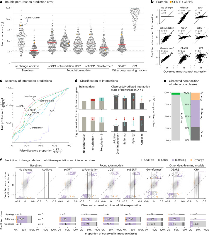
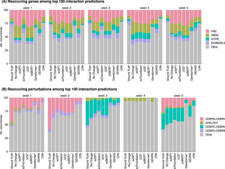
- In the double perturbation benchmark on Norman et al. data (100 single genes, 124 gene pairs, 19,264 genes), all models had prediction error substantially higher than the additive baseline, and none was better than the “no change” baseline for genetic interaction prediction. Using the full dataset, the authors identified 5,035 genetic interactions out of potentially 124,000 at a 5% false discovery rate.
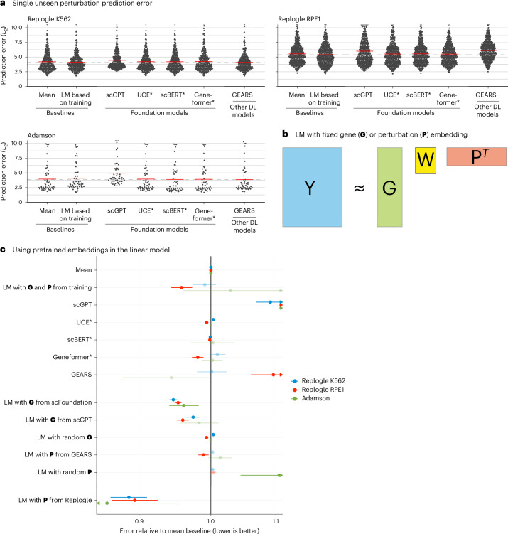
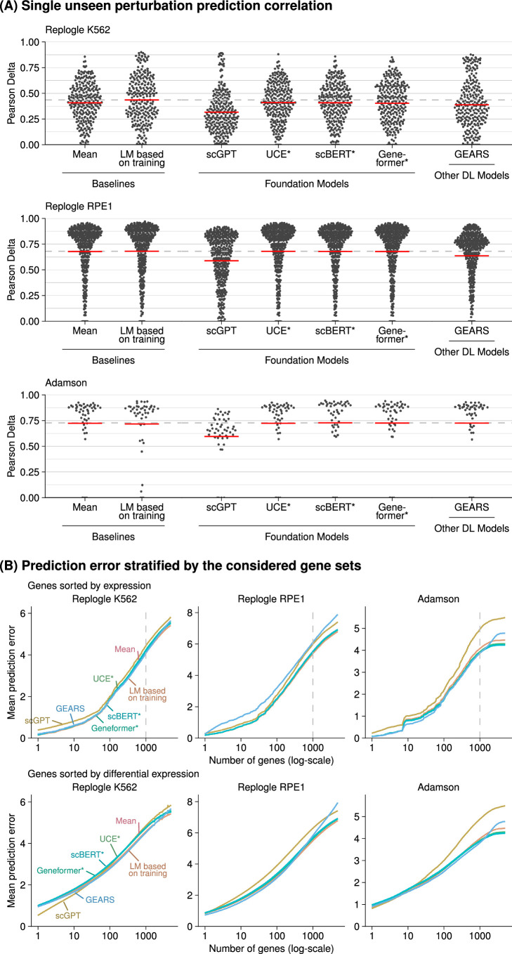
- In the unseen single perturbation benchmark, none of the deep learning models consistently outperformed the mean prediction or the linear model. A linear model with perturbation embeddings pretrained on Replogle data consistently outperformed all other models; gene embeddings from scFoundation and scGPT outperformed the mean baseline but did not consistently outperform the linear model using G and P from the training data.
- All models mostly predicted buffering interactions, rarely predicted synergistic interactions, and even more rarely predicted them correctly. For most genes, scGPT, UCE and scBERT predictions did not vary across perturbations, and GEARS and scFoundation predictions varied considerably less than the ground truth.
Methods
- Benchmarked GEARS v0.1.2, scGPT v0.2.1, scFoundation, CPA v0.8.8, Geneformer v0.1.0, scBERT and UCE against simple baselines. Double perturbation analysis used Norman et al. data, training on all 100 single perturbations and 62 double perturbations and testing on the remaining 62 double perturbations across five random splits. Single perturbation analysis used Adamson et al. and Replogle et al. K562/RPE1 datasets with GEARS’ simulation test–training splitting repeated twice.
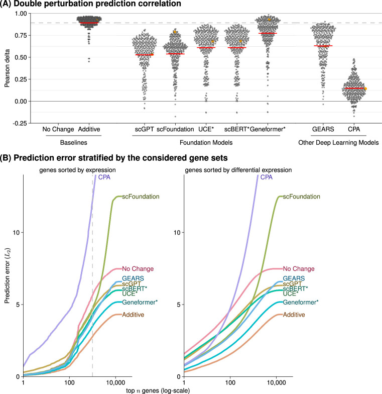
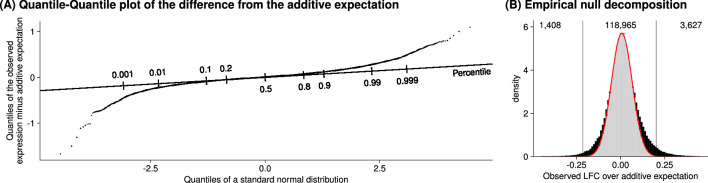
- Prediction error was the L2 distance between predicted and observed expression for the 1,000 most highly expressed genes; Pearson delta and other gene subsets were also examined. Genetic interactions were defined as deviations from additive expectation using Efron’s empirical null approach with the locfdr package at a 5% false discovery rate, and true-positive rate versus false discovery proportion curves were computed.
- The linear model represented read-out genes with matrix G and perturbations with matrix P, found W via normal equations with ridge penalty λ = 0.1, and used K = 10. Baselines included “no change,” “additive” and “mean.” For Geneformer, UCE and scBERT, a ridge regression linear decoder mapped perturbed embeddings to gene expression.
Limitations
- The paper states that only four datasets were used, chosen because they were used in the publications presenting GEARS, scGPT and scFoundation; all datasets are from cancer cell lines; and the authors did not attempt to improve original quality control, for example by excluding perturbations that did not affect their own target gene.
- The paper acknowledges that for UCE and scBERT, the post-perturbation embedding was calculated by overwriting rows for perturbed genes with values from the ground truth expression matrix, so test data leakage could theoretically give those models an advantage. It also notes that CPA authors submitted a code fix, but because the new code had worse performance, the original code results are reported.
Model-written summary. Check it against the paper before relying on it.
Integrity signals
Registry
Cites
Statistics
Figures





Verification
Claims the paper makes
6 Valid · 0 Not valid · 5 Not checked · 32 Own results and interpretations
Every source the paper cites for this claim was checked and supports it.
In the paper
“The approach that did consistently outperform all other models was a linear model with P pretrained on the Replogle data (using the K562 cell line data as pretraining for the Adamson and RPE1 data and the RPE1 cell line for the K562 data).”
§ Deep-learning-based gene perturbation effect prediction does not yet outperform simple linear baselines > Main
What the sources say
- Supportedcites Replogle et al.13 Replogle, J. M. et al. Mapping information-rich genotype-phenotype landscapes with genome-scale Perturb-seq. Cell 185, 2559–2575 (2022). source
The Methods describe Perturb-seq datasets generated in K562 and RPE1 cells, confirming that this paper is the source of the identified Replogle data. The statement that a pretrained linear model outperformed other models is the citing authors’ comparison, not a result attributed to Replogle et al. (LLM, conf=0.88)
plain- Asserted: passes — The authors put it forward as true.
- Checkable: passes — It can be checked against evidence.
- Load-bearing: passes — The paper’s conclusions depend on it.
- Based: passes — The paper gives a reason why it holds.
- Supported
The cited sources support only part of this claim — read each source’s verdict below.
In the paper
“Since the release of our paper as a preprint, several other benchmarks15,16,22–27 were released that also show that deep learning models struggle to outperform simple baselines.”
§ Deep-learning-based gene perturbation effect prediction does not yet outperform simple linear baselines > Main
What the sources say
- Supportedcites [15] Kernfeld, E., Yang, Y., Weinstock, J. S., Battle, A. & Cahan, P. A systematic comparison of computational methods for expression forecasting. Preprint at bioRxiv https://doi.org/10.1101/2023.07.28.551039 (2024). sourceExperimental — accuracy not yet measured
The Discussion reports that very simple baselines typically performed at least as well as the methods benchmarked. This paper is one of the benchmarks cited in the sentence; it need not itself establish the findings of the other cited benchmarks. (LLM, conf=0.90)
- Supportedcites [16] Csendes, G., Sanz, G., Szalay, K. Z. & Szalai, B. Benchmarking foundation cell models for post-perturbation RNA-seq prediction. BMC Genomics 26, 393 (2025). sourceExperimental — accuracy not yet measured
The Discussion reports that this benchmark compared foundation models with baselines and found that the simple Train Mean model outperformed scGPT and scFoundation in most cases. The source therefore supports its use as one example among the cited benchmarks; it does not, by itself, establish what the other benchmarks found. (LLM, conf=0.91)
- Not checked — no full text of the sourcecites [22] Wenteler, A. et al. PertEval-scFM: benchmarking single-cell foundation models for perturbation effect prediction. In Proc. 42nd International Conference on Machine Learning (ICML, 2025). source
- Supportedcites [23] Bendidi, I. et al. Benchmarking transcriptomics foundation models for perturbation analysis: one PCA still rules them all. Preprint at https://arxiv.org/abs/2410.13956 (2024). source
This source is a benchmark comparing transcriptomics foundation models with simpler baselines. Its Conclusion (section 6) reports that scVI and PCA outperform the foundation models on most perturbation-related tasks, supporting its use as an example of the benchmarks cited. The timing relative to the citing authors’ preprint is their framing, not a finding attributed to this source. (LLM, conf=0.91)
- Supportedcites [24] Wu, Y. et al. PerturBench: benchmarking machine learning models for cellular perturbation analysis. Preprint at https://arxiv.org/abs/2408.10609 (2024). source
The Introduction reports that simple architectures can outperform more sophisticated models on larger datasets. Section 6 (Discussion) likewise says the Latent Additive and Decoder-Only baselines outperform more complex methods on larger datasets, while acknowledging that the complex methods perform best on some smaller datasets. This supports the claim that deep learning models can struggle to outperform simple baselines; the timing of the benchmark's release is the citing authors' framing. (LLM, conf=0.91)
- Partly supportedcites [25] Li, L. et al. A systematic comparison of single-cell perturbation response prediction models. Preprint at bioRxiv https://doi.org/10.1101/2024.12.23.630036 (2024). sourceExperimental — accuracy not yet measured
The Abstract identifies this paper as a benchmark comparing methods and baselines and reports limits to model performance. It does not say that deep-learning models struggled to outperform simple baselines, so the specific finding attributed to this benchmark is not supported by our copy. (LLM, conf=0.78)
- Not checked — no full text of the sourcecites [26] Li, C. et al. Benchmarking AI models for in silico gene perturbation of cells. Preprint at bioRxiv https://doi.org/10.1101/2024.12.20.629581 (2025). source
- Supportedcites [27] Wong, D. R., Hill, A. S. & Moccia, R. Simple controls exceed best deep learning algorithms and reveal foundation model effectiveness for predicting genetic perturbations. Bioinformatics 41, btaf317 (2025). sourceExperimental — accuracy not yet measured
The Abstract (Results) says this paper's simple baseline outperforms state-of-the-art deep-learning methods. Section 3.1 reports that the CRISPR-informed mean model performed better on average than all deep-learning models tested, while acknowledging conditions in which deep-learning models did better. It therefore supports the citing sentence as one of the benchmarks showing that deep-learning models struggle to outperform simple baselines. (LLM, conf=0.91)
plain- Asserted: passes — The authors put it forward as true.
- Checkable: passes — It can be checked against evidence.
- Load-bearing: unclear — It is unclear whether the paper’s conclusions depend on it.
- Based: passes — The paper gives a reason why it holds.
- Supported
Every source the paper cites for this claim was checked and supports it.
In the paper
“Using the full dataset, we identified 5,035 genetic interactions (out of potentially 124,000) at a false discovery rate of 5%.”
§ Deep-learning-based gene perturbation effect prediction does not yet outperform simple linear baselines > Main
What the sources say
- Supportedcites Norman et al.11 Norman, T. M. et al. Exploring genetic interaction manifolds constructed from rich single-cell phenotypes. Science 365, 786–793 (2019). source
The ‘An overexpression strategy identifies strong genetic interactions’ section (page unavailable) describes Norman et al.’s genetic-interaction dataset, supporting its identification as the dataset used. The 5,035 interactions, 124,000 potential interactions, and 5% false-discovery rate are presented as the citing authors’ own analysis (‘we identified’), not as findings attributed to Norman et al.; the cited paper does not report those figures. (LLM, conf=0.84)
plain- Asserted: passes — The authors put it forward as true.
- Checkable: passes — It can be checked against evidence.
- Load-bearing: unclear — It is unclear whether the paper’s conclusions depend on it.
- Based: passes — The paper gives a reason why it holds.
- Supported
Every source the paper cites for this claim was checked and supports it.
In the paper
“Another limitation is that all datasets are from cancer cell lines, which, for example, Theodoris et al.5 excluded from their training data because of concerns about their high mutational burden.”
§ Deep-learning-based gene perturbation effect prediction does not yet outperform simple linear baselines > Main
What the sources say
- Supportedcites Theodoris et al.5 Theodoris, C. V. et al. Transfer learning enables predictions in network biology. Nature 618, 616–624 (2023). source
The Geneformer architecture and pretraining section states that Theodoris et al. excluded cells with high mutational burdens, including immortalized cell lines, from their pretraining corpus because mutations could substantially rewire networks. The cited paper does not establish that all datasets in the citing authors’ benchmark came from cancer cell lines; that is the citing authors’ own description, not the point attributed to this source. (LLM, conf=0.94)
plain- Asserted: passes — The authors put it forward as true.
- Checkable: passes — It can be checked against evidence.
- Load-bearing: unclear — It is unclear whether the paper’s conclusions depend on it.
- Based: passes — The paper gives a reason why it holds.
- Supported
A result the paper reports from its own data — it cites no other source for it, so there is none to check. The quote shows it is in the paper.
In the paper
“all models except Geneformer and scFoundation predicted LFC ≈ 0—like the ‘no change’ baseline—for the double perturbation of these two genes, despite their strong individual effects (Extended Data Fig. 6).”
§ Deep-learning-based gene perturbation effect prediction does not yet outperform simple linear baselines > Main
plain- Asserted: passes — The authors put it forward as true.
- Checkable: passes — It can be checked against evidence.
- Load-bearing: unclear — It is unclear whether the paper’s conclusions depend on it.
- Based: passes — The paper gives a reason why it holds.
22 more claims
Create a free account to see all 43 claims and to verify the 2 references still open.
- Probably not a substantial claim. 15
- It may state two separate claims as one. 3
Claims other papers make about this one
Each is checked against this paper’s own text: does it say what the citing paper says it does?
The cited source says what the claim attributes to it.
In the citing paper
“Besides, simple baselines proved highly competitive with complex deep learning models, which is consistent with a previous study (25).”
From A systematic comparison of single-cell perturbation response prediction models (2026) · cites this paper as [25]
The cited source says what the claim attributes to it.
In the citing paper
“This finding extends recent observations that simple additive or linear baselines remain difficult to outperform in double-perturbation prediction (25, 31).”
From A systematic comparison of single-cell perturbation response prediction models (2026) · cites this paper as [25]
The cited source says what the claim attributes to it.
In the citing paper
“Recent studies have provided initial benchmarks comparing foundation models, other deep learning architectures, and simple baselines for perturbation effect prediction and reported that complex models do not consistently outperform the simpler alternatives (22–26).”
From A systematic comparison of single-cell perturbation response prediction models (2026) · cites this paper as [25]
The cited source says what the claim attributes to it.
In the citing paper
“While this work provides valuable insights, its evaluation was limited in dataset diversity and task coverage, leaving the question of whether such conclusions generalize across broader biological contexts.”
From A systematic comparison of single-cell perturbation response prediction models (2026) · cites this paper as [25]
Citations
Cites
The igraph software package for complex network research
Csárdi, G., & Nepusz, T. (2006) · Medical Entomology and Zoology · Cited by 13,507
A Survey on Evaluation of Large Language Models
Chang, Y., Wang, X., Wang, J., Wu, Y., Yang, L., Zhu, K., Chen, H., Yi, X., Wang, C., Wang, Y., et al. (2024) · ACM Transactions on Intelligent Systems and Technology · doi:10.1145/3641289 · Cited by 4,254
The Gene Ontology knowledgebase in 2023
The Gene Ontology Consortium, Aleksander, S. A., Balhoff, J., Carbon, S., Cherry, J. M., Drabkin, H. J., Ebert, D., Feuermann, M., Gaudet, P., Harris, N. L., et al. (2023) · GENETICS · doi:10.1093/genetics/iyad031 · Cited by 2,664
Regev, A., Teichmann, S. A., Lander, E. S., Amit, I., Benoist, C., Birney, E., Bodenmiller, B., Campbell, P., Carninci, P., Clatworthy, M., et al. (2017) · eLife · doi:10.7554/elife.27041 · Cited by 2,232
scGPT: Towards Building a Foundation Model for Single-Cell Multi-omics Using Generative AI
Cui, H., Wang, C., Maan, H., Pang, K., Luo, F., & Wang, B. (2023) · doi:10.1101/2023.04.30.538439 · Cited by 1,694
Benchmarking atlas-level data integration in single-cell genomics
Luecken, M. D., Büttner, M., Chaichoompu, K., Danese, A., Interlandi, M., Mueller, M. F., Strobl, D. C., Zappia, L., Dugas, M., Colomé-Tatché, M., et al. (2022) · Nature Methods · doi:10.1038/s41592-021-01336-8 · Cited by 1,438
Adamson, B., Norman, T. M., Jost, M., Cho, M. Y., Nuñez, J. K., Chen, Y., Villalta, J. E., Gilbert, L. A., Horlbeck, M. A., Hein, M. Y., et al. (2016) · Cell · doi:10.1016/j.cell.2016.11.048 · Cited by 1,193
Transfer learning enables predictions in network biology
Theodoris, C. V., Xiao, L., Chopra, A., Chaffin, M. D., Al Sayed, Z. R., Hill, M. C., Mantineo, H., Brydon, E. M., Zeng, Z., Liu, X. S., et al. (2023) · Nature · doi:10.1038/s41586-023-06139-9 · Cited by 1,193 · cited 1×
“Another limitation is that all datasets are from cancer cell lines, which, for example, Theodoris et al. 5 excluded from their training data because of concerns about their high mutational burden.”
Large-Scale Inference: Empirical Bayes Methods for Estimation, Testing, and Prediction
Efron, B. (2010) · Cambridge University Press eBooks · doi:10.1017/cbo9780511761362 · Cited by 813
Mapping information-rich genotype-phenotype landscapes with genome-scale Perturb-seq
Replogle, J. M., Saunders, R. A., Pogson, A. N., Hussmann, J. A., Lenail, A., Guna, A., Mascibroda, L., Wagner, E. J., Adelman, K., Lithwick-Yanai, G., et al. (2022) · Cell · doi:10.1016/j.cell.2022.05.013 · Cited by 795 · cited 2×
“For the single gene perturbation benchmarks, we used the data from Adamson et al. 14 and Replogle et al. 13 as provided by GEARS (details in ‘Data availability’).”
Research works printed but not linked: 1
- Märtens, K., Donovan-Maiye, R. & Ferkinghoff-Borg, J. Enhancing generative perturbation models with LLM-informed gene embeddings. In Proc. Workshop on Machine Learning for Genomics Explorations (ICLR, 2024). https://openreview.net/forum?id=eb3ndUlkt4
Cited by
Predicting cellular responses to perturbation across diverse contexts with State
Adduri, A. K., Gautam, D., Bevilacqua, B., Naghipourfar, M., Imran, A., Shah, R., Teyssier, N., Verma, R., Carpenter, C., Eraslan, B., et al. (2026) · Cell · doi:10.1016/j.cell.2026.07.052 · Cited by 100
PerturbNet predicts single-cell responses to unseen chemical and genetic perturbations
Yu, H., Qian, W., Song, Y., & Welch, J. D. (2025) · Molecular Systems Biology · doi:10.1038/s44320-025-00131-3 · Cited by 57
Viñas Torné, R., Wiatrak, M., Piran, Z., Fan, S., Jiang, L., Teichmann, S. A., Nitzan, M., & Brbić, M. (2026) · Nature Biotechnology · doi:10.1038/s41587-025-02777-8 · Cited by 58
Benchmarking foundation cell models for post-perturbation RNA-seq prediction
Csendes, G., Sanz, G., Szalay, K. Z., & Szalai, B. (2025) · BMC Genomics · doi:10.1186/s12864-025-11600-2 · Cited by 47
Ma, C., Zhang, H., Rao, Y., Jiang, X., Liu, B., Sun, Z., Song, Z., Gao, Y., Cui, Y., Liu, X., et al. (2025) · npj Digital Medicine · doi:10.1038/s41746-025-02198-6 · Cited by 71
Metadata
- Authors
- Ahlmann-Eltze, C., Huber, W., & Anders, S.
- Affiliations
- Heidelberg University (DE)
- European Molecular Biology Laboratory (DE)
- Corresponding author
- Ahlmann-Eltze, Constantin
- Venue
- Nature Methods
- Published
- 2025-08
- Volume
- 22
- Issue
- 8
- Pages
- 1657-1661
- ISSN
- 1548-7091 (ISSN-L)
- 1548-7105
- PMC
- PMC12328236
- OpenAlex
- W4412929241
- Cited by
- 238
- References
- 31
- Citations by year
- 2026: 147 · 2025: 78
- FWCI
- 67.16
- Type
- journal article
- Language
- en
- Open access
- hybrid
- doi.org
- Licence
- cc-by
- creativecommons.org/licenses/by/4.0 (tdm)
- creativecommons.org/licenses/by/4.0 (vor, 3 d)
- Locations
- Nature Methods (publishedVersion, cc-by)
- bioRxiv (Cold Spring Harbor Laboratory) (acceptedVersion, cc-by-nc)
- PubMed Central (publishedVersion, cc-by)
- PubMed (publishedVersion)
- Funders
- Klaus Tschira Stiftung (00.022.2019)
- Topics
- Life Sciences › Biochemistry, Genetics and Molecular Biology › Molecular Biology › Single-cell and spatial transcriptomics
- Life Sciences › Biochemistry, Genetics and Molecular Biology › Molecular Biology › Gene Regulatory Network Analysis
- Life Sciences › Biochemistry, Genetics and Molecular Biology › Molecular Biology › Bioinformatics and Genomic Networks
- Keywords
- single-cell transcriptomics, foundation models, deep learning, benchmarking, transcriptome changes
- MeSH terms
- Deep Learning, Algorithms, Humans, Computational Biology, Gene Expression Profiling, Single-Cell Analysis, Transcriptome
About these checks
Registry, retraction, Cites and statistics results are computed, not judged, with one exception: a printed reference that no index lists is read once by a model before it counts as a citation error. Claims are extracted by a model and kept only when their quote appears verbatim in the text; each cited source is then checked, with a model’s help, for whether it says what the claim relies on. Those verdicts can be wrong — read the claim’s quote and the cited source before relying on one.
The claim verdicts this report counts are experimental: their accuracy is not yet measured.
A language model drew the claims from the paper on 2026-10-10, under version 3 of the claim definition (model deepseek-v4.1-flash, prompt extract-v3).
A second model labelled each claim on 2026-10-10 (model jev-1.13-20260917, definition revision gold-guideline-v0.2).
Cited sources are checked with a language model’s help (gpt-6-sol).
Statistics and arithmetic are recomputed, not judged.
Confidence bands are shown only for fields calibrated on our annotated test set. None is calibrated yet, so no band is shown.
What counts as a claim ›How we measure confidence ›How we check this ›
Are you an author, or do you see a problem with this page? Request a review
How to cite
Cite CoChat for the checks on this page, and the paper for its own findings.
- This page
- CoChat. (2026). Citation check: Deep-learning-based gene perturbation effect prediction does not yet outperform simple linear baselines. https://app.cochat.ai/papers/10.1038/s41592-025-02772-6
- The paper
- Ahlmann-Eltze, C., Huber, W., & Anders, S. (2025). Deep-learning-based gene perturbation effect prediction does not yet outperform simple linear baselines. Nature Methods. https://doi.org/10.1038/s41592-025-02772-6
Data sources
Bibliographic data: Semantic Scholar, OpenAlex, Crossref.
Contains information from the Semantic Scholar Academic Graph Datasets, made available under the ODC Attribution License (ODC-BY 1.0).
Semantic Scholar’s data is described in: Kinney, R., et al. (2023). The Semantic Scholar Open Data Platform. arXiv:2301.10140.
