

Climate models predict increasing temperature variability in poor countries
Open accessThe DOI matches its Crossref record; 56 of the 56 references it cites were found in a registry or an index.
Abstract
Temperature variability will increase in poor countries and decrease in rich countries, creating a new climate injustice.
Overview
The claims and statistics of this paper haven’t been checked yet.
Free: it reads the open-access text and checks the first 5 claims that cite a source we can check. Create a free account to check every claim.
Integrity signals
Registry
Cites
Statistics
Figures
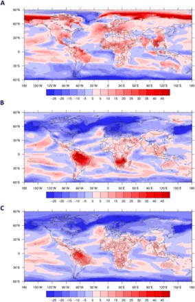
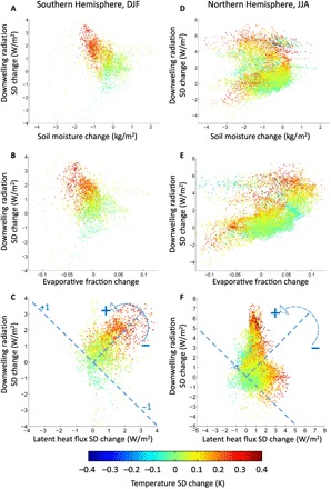
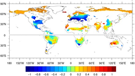
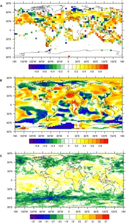
Verification
Claims the paper makes
The claims and statistics of this paper haven’t been checked yet.
Free: it reads the open-access text and checks the first 5 claims that cite a source we can check. Create a free account to check every claim.
Claims other papers make about this one
Each is checked against this paper’s own text: does it say what the citing paper says it does?
The cited source says what the claim attributes to it.
In the citing paper
“This is clearly seen in poor countries, which are more vulnerable to weather and climate fluctuation than wealthier countries (95).”
From The Impact of Climate Change on Mental Health: A Systematic Descriptive Review (2020) · cites this paper as [95]
Self-check
Percentages, sums and reported differences re-computed from the paper’s own numbers.
The self-check needs the paper’s full text.
Citations
Cites
The ERA‐Interim reanalysis: configuration and performance of the data assimilation system
Dee, D. P., Uppala, S. M., Simmons, A. J., Berrisford, P., Poli, P., Kobayashi, S., Andrae, U., Balmaseda, M. A., Balsamo, G., Bauer, P., et al. (2011) · Quarterly Journal of the Royal Meteorological Society · doi:10.1002/qj.828 · Cited by 24,480
An Overview of CMIP5 and the Experiment Design
Taylor, K. E., Stouffer, R. J., & Meehl, G. A. (2012) · Bulletin of the American Meteorological Society · doi:10.1175/bams-d-11-00094.1 · Cited by 14,052
The Modern-Era Retrospective Analysis for Research and Applications, Version 2 (MERRA-2)
Gelaro, R., McCarty, W., Suárez, M. J., Todling, R., Molod, A., Takacs, L., Randles, C. A., Darmenov, A., Bosilovich, M. G., Reichle, R., et al. (2017) · Journal of Climate · doi:10.1175/jcli-d-16-0758.1 · Cited by 9,010
NCEP–DOE AMIP-II reanalysis (R-2)
Kanamitsu, M., Ebisuzaki, W., Woollen, J., Yang, S.-K., Hnilo, J. J., Fiorino, M., & Potter, G. L. (2002) · Bulletin of the American Meteorological Society · doi:10.1175/bams-83-11-1631 · Cited by 5,771
Investigating soil moisture–climate interactions in a changing climate: A review
Seneviratne, S. I., Corti, T., Davin, E. L., Hirschi, M., Jaeger, E. B., Lehner, I., Orlowsky, B., & Teuling, A. J. (2010) · Earth-Science Reviews · doi:10.1016/j.earscirev.2010.02.004 · Cited by 5,638
Climate Extremes: Observations, Modeling, and Impacts
Easterling, D. R., Meehl, G. A., Parmesan, C., Changnon, S. A., Karl, T. R., & Mearns, L. O. (2000) · Science · doi:10.1126/science.289.5487.2068 · Cited by 4,867
Tipping elements in the Earth’s climate system
Lenton, T. M., Held, H., Kriegler, E., Hall, J. W., Lucht, W., Rahmstorf, S., & Schellnhuber, H. J. (2008) · Proceedings of the National Academy of Sciences · doi:10.1073/pnas.0705414105 · Cited by 3,982
Self-citationThe RCP greenhouse gas concentrations and their extensions from 1765 to 2300
Meinshausen, M., Smith, S. J., Calvin, K., Daniel, J. S., Kainuma, M. L. T., Lamarque, J.-F., Matsumoto, K., Montzka, S. A., Raper, S. C. B., Riahi, K., et al. (2011) · Climatic Change · doi:10.1007/s10584-011-0156-z · Cited by 3,584
The Twentieth Century Reanalysis Project
Compo, G. P., Whitaker, J. S., Sardeshmukh, P. D., Matsui, N., Allan, R. J., Yin, X., Gleason, B. E., Vose, R. S., Rutledge, G., Bessemoulin, P., et al. (2011) · Quarterly Journal of the Royal Meteorological Society · doi:10.1002/qj.776 · Cited by 3,518
Global surface temperature change
Hansen, J., Ruedy, R., Sato, M., & Lo, K. (2010) · Reviews of Geophysics · doi:10.1029/2010rg000345 · Cited by 3,081
Research works printed but not linked: 1
- 10.1175/1520-0442(2002)015 · doi:10.1175/1520-0442(2002)015
Cited by
Weather and Climate Extreme Events in a Changing Climate
(2023) · Climate Change 2021 – The Physical Science Basis · doi:10.1017/9781009157896.013 · Cited by 1,784
The Impact of Climate Change on Mental Health: A Systematic Descriptive Review
Cianconi, P., Betrò, S., & Janiri, L. (2020) · Frontiers in Psychiatry · doi:10.3389/fpsyt.2020.00074 · Cited by 1,320
“This loss is linked to a decrease on economic growth leading to a long-term economic disadvantage and promoting political instability and conflicts (95).”
BackgroundProgress and Expectation of Atmospheric Water Harvesting
Tu, Y., Wang, R., Zhang, Y., & Wang, J. (2018) · Joule · doi:10.1016/j.joule.2018.07.015 · Cited by 762
Climate change and the need for agricultural adaptation
Anderson, R., Bayer, P. E., & Edwards, D. (2020) · Current Opinion in Plant Biology · doi:10.1016/j.pbi.2019.12.006 · Cited by 543
Towards food supply chain resilience to environmental shocks
Davis, K. F., Downs, S., & Gephart, J. A. (2020) · Nature Food · doi:10.1038/s43016-020-00196-3 · Cited by 501
Revised Estimates of the Impact of Climate Change on Extreme Poverty by 2030
Jafino, B. A., Walsh, B., Rozenberg, J., & Hallegatte, S. (2020) · World Bank, Washington, DC eBooks · doi:10.1596/1813-9450-9417 · Cited by 556
Climate change, ecosystems and abrupt change: science priorities
Turner, M. G., Calder, W. J., Cumming, G. S., Hughes, T. P., Jentsch, A., LaDeau, S. L., Lenton, T. M., Shuman, B. N., Turetsky, M. R., Ratajczak, Z., et al. (2020) · Philosophical Transactions of the Royal Society B: Biological Sciences · doi:10.1098/rstb.2019.0105 · Cited by 382
Self-citationStrengthening and Implementing the Global Response
(2022) · Global Warming of 1.5°C · doi:10.1017/9781009157940.006 · Cited by 352
Green spaces provide substantial but unequal urban cooling globally
Li, Y., Svenning, J.-C., Zhou, W., Zhu, K., Abrams, J. F., Lenton, T. M., Ripple, W. J., Yu, Z., Teng, S. N., Dunn, R. R., et al. (2024) · Nature Communications · doi:10.1038/s41467-024-51355-0 · Cited by 292
Self-citationGlobal Inequality in Cooling from Urban Green Spaces and its Climate Change Adaptation Potential
Li, Y., Svenning, J.-C., Zhou, W., Zhu, K., Abrams, J. F., Lenton, T. M., Teng, S. N., Dunn, R. R., & Xu, C. (2023) · arXiv · doi:10.48550/arxiv.2307.09725 · Cited by 366
Self-citationHase, V., Mahl, D., Schäfer, M. S., & Keller, T. R. (2021) · Global Environmental Change · doi:10.1016/j.gloenvcha.2021.102353 · Cited by 275
“These adverse consequences are borne disproportionately by less industrialized countries in Africa, Asia, or Latin America (Althor et al., 2016; Bathiany et al., 2018; United Nations Framework Convention on Climate Change, 2007).”
BackgroundAnthropogenically-driven increases in the risks of summertime compound hot extremes
Wang, J., Chen, Y., Tett, S. F. B., Yan, Z., Zhai, P., Feng, J., & Xia, J. (2020) · Nature Communications · doi:10.1038/s41467-019-14233-8 · Cited by 324
The need for bottom-up assessments of climate risks and adaptation in climate-sensitive regions
Conway, D., Nicholls, R. J., Brown, S., Tebboth, M. G. L., Adger, W. N., Ahmad, B., Biemans, H., Crick, F., Lutz, A. F., De Campos, R. S., et al. (2019) · Nature Climate Change · doi:10.1038/s41558-019-0502-0 · Cited by 256
Global population exposure to landscape fire air pollution from 2000 to 2019
Xu, R., Ye, T., Yue, X., Yang, Z., Yu, W., Zhang, Y., Bell, M. L., Morawska, L., Yu, P., Zhang, Y., et al. (2023) · Nature · doi:10.1038/s41586-023-06398-6 · Cited by 230
“…the increasing severity and frequency of wildfires are related to anthropogenic climate change 1–4 , our finding about the socioeconomic disparities provides further evidence of climate injustice, that is, those least responsible for climate change suffer the most from its consequences 38,39 .”
Wellbeing economy: An effective paradigm to mainstream post-growth policies?
Fioramonti, L., Coscieme, L., Costanza, R., Kubiszewski, I., Trebeck, K., Wallis, S., Roberts, D., Mortensen, L. F., Pickett, K. E., Wilkinson, R., et al. (2022) · Ecological Economics · doi:10.1016/j.ecolecon.2021.107261 · Cited by 199
Outdoor Personal Thermal Management with Simultaneous Electricity Generation
Luo, H., Zhu, Y., Xu, Z., Hong, Y., Ghosh, P., Kaur, S., Wu, M., Yang, C., Qiu, M., & Li, Q. (2021) · Nano Letters · doi:10.1021/acs.nanolett.1c00400 · Cited by 230
Climate Change and Children’s Mental Health: A Developmental Perspective
Vergunst, F., & Berry, H. L. (2022) · Clinical Psychological Science · doi:10.1177/21677026211040787 · Cited by 197
Linking Global to Regional Climate Change
(2023) · Climate Change 2021 – The Physical Science Basis · doi:10.1017/9781009157896.012 · Cited by 176
Gimeno, L., Vázquez, M., Eiras-Barca, J., Sorí, R., Stojanovic, M., Algarra, I., Nieto, R., Ramos, A. M., Durán-Quesada, A. M., & Dominguez, F. (2020) · Earth-Science Reviews · doi:10.1016/j.earscirev.2019.103070 · Cited by 200
Heat Exposure and Occupational Injuries: Review of the Literature and Implications
Spector, J. T., Masuda, Y. J., Wolff, N. H., Calkins, M., & Seixas, N. (2019) · Current Environmental Health Reports · doi:10.1007/s40572-019-00250-8 · Cited by 176
Sustainable Development, Poverty Eradication and Reducing Inequalities
(2022) · Global Warming of 1.5°C · doi:10.1017/9781009157940.007 · Cited by 178
Macroeconomic and Financial Policies for Climate Change Mitigation: A Review of the Literature
Krogstrup, S., & Oman, W. (2019) · IMF Working Paper · doi:10.5089/9781513511955.001 · Cited by 253
Climate change and mental health research methods, gaps, and priorities: a scoping review
Hwong, A. R., Wang, M., Khan, H., Chagwedera, D. N., Grzenda, A., Doty, B., Benton, T., Alpert, J., Clarke, D., & Compton, W. M. (2022) · The Lancet Planetary Health · doi:10.1016/s2542-5196(22)00012-2 · Cited by 154
Specialisation, diversification and the ladder of green technology development
Perruchas, F., Consoli, D., & Barbieri, N. (2020) · Research Policy · doi:10.1016/j.respol.2020.103922 · Cited by 166
“Further, while environmentallyfriendly technologies emerge first, and more frequently, in more developed countries the urgency of effective deployment to adapt to climate change is stronger in poorer countries (Mendelsohn et al., 2006; Bathiany et al., 2018)(1).”
The importance of species interactions in eco-evolutionary community dynamics under climate change
Åkesson, A., Curtsdotter, A., Eklöf, A., Ebenman, B., Norberg, J., & Barabás, G. (2021) · Nature Communications · doi:10.1038/s41467-021-24977-x · Cited by 180
Local mechanisms for global daytime, nighttime, and compound heatwaves
Wu, S., Luo, M., Zhao, R., Li, J., Sun, P., Liu, Z., Wang, X., Wang, P., & Zhang, H. (2023) · npj Climate and Atmospheric Science · doi:10.1038/s41612-023-00365-8 · Cited by 175
Tropical and Boreal Forest – Atmosphere Interactions: A Review
Artaxo, P. E., Hansson, H., Andreae, M. O., Bäck, J. K., Alves, E. G., Barbosa, H. M. J., Bender, F. A. ‐., Bourtsoukidis, E., Carbone, S., Chi, J., et al. (2022) · Tellus B · doi:10.16993/tellusb.34 · Cited by 164
Climate damage projections beyond annual temperature
Waidelich, P., Batıbeniz, F., Rising, J., Kikstra, J., & Seneviratne, S. I. (2024) · Nature Climate Change · doi:10.1038/s41558-024-01990-8 · Cited by 175
“Continued global warming is expected to exacerbate these trends, potentially with uneven impacts across regions 5,9,10 .”
Supply-chain data sharing for scope 3 emissions
Stenzel, A., & Waichman, I. (2023) · npj Climate Action · doi:10.1038/s44168-023-00032-x · Cited by 175
Integrating regional and interregional approaches to identify ecological security patterns
Dong, J., Peng, J., Xu, Z., Liu, Y., Wang, X., & Li, B. (2021) · Landscape Ecology · doi:10.1007/s10980-021-01233-7 · Cited by 136
Regime shifts, trends, and variability of lake productivity at a global scale
Gilarranz, L. J., Narwani, A., Odermatt, D., Siber, R., & Dakos, V. (2022) · Proceedings of the National Academy of Sciences · doi:10.1073/pnas.2116413119 · Cited by 141
Self-citationClimate Econometrics: Can the Panel Approach Account for Long‐Run Adaptation?
Mérel, P., & Gammans, M. (2021) · American Journal of Agricultural Economics · doi:10.1111/ajae.12200 · Cited by 147
Luo, M., Wu, S., Lau, G. N., Pei, T., Liu, Z., Wang, X., Ning, G., Chan, T. O., Yang, Y., & Zhang, W. (2024) · Science Advances · doi:10.1126/sciadv.adl1598 · Cited by 146
“This tracking identifies extreme events in all seasons of the calendar year, and we focus on examining the events in the hot summer season only, which is defined as June- July-August (JJA) for the Northern Hemisphere and December- January-February (DJF) for the Southern Hemisphere ( 52 , 53 ).”
BackgroundTemporary migration and climate variation in eastern Africa
Mueller, V., Sheriff, G. D., Dou, X., & Gray, C. (2019) · World Development · doi:10.1016/j.worlddev.2019.104704 · Cited by 149
“Africa is likely to experience warming and increased climate variability by the late 21st century (IPCC, 2013; Bathiany et al., 2018).”
BackgroundFiscal Policies for Development and Climate Action
Pigato, M. A. (2018) · World Bank, Washington, DC eBooks · doi:10.1596/978-1-4648-1358-0 · Cited by 151
Population growth and climate change: addressing the overlooked threat multiplier
Dodson, J. C., Dérer, P., Cafaro, P., & Götmark, F. (2020) · Science of The Total Environment · doi:10.1016/j.scitotenv.2020.141346 · Cited by 122
“…growth as a key driver of future climate risk (Asefi-Najafabady et al., 2018; Jones et al., 2015; Liu et al., 2017), particularly in less-developed countries that have contributed the least to climate change but maintain growing populations (Ahmadalipour et al., 2019; Bathiany et al., 2018).”
BackgroundClimate-mediated shifts in temperature fluctuations promote extinction risk
Duffy, K. M., Gouhier, T. C., & Ganguly, A. R. (2022) · Nature Climate Change · doi:10.1038/s41558-022-01490-7 · Cited by 120
Dynamical and thermodynamical drivers of variability in European summer heat extremes
Suarez‐Gutierrez, L., Müller, W. A., Li, C., & Marotzke, J. (2020) · Climate Dynamics · doi:10.1007/s00382-020-05233-2 · Cited by 121
Widlansky, M. J., Long, X., & Schloesser, F. (2020) · Communications Earth & Environment · doi:10.1038/s43247-020-0008-8 · Cited by 121
Climate change and mental health research methods, gaps, and priorities: a scoping reviewPreprint
Hwong, A. R. (2022) · doi:10.17605/osf.io/xr9ut · Cited by 112
Accelerating upward treeline shift in the Altai Mountains under last-century climate change
Gatti, R. C., Callaghan, T. V., Velichevskaya, A. I., Dudko, A., Fabbio, L., Battipaglia, G., & Liang, J. (2019) · Scientific Reports · doi:10.1038/s41598-019-44188-1 · Cited by 122
Sensitivity of grain yields to historical climate variability in India
Davis, K. F., Chhatre, A., Rao, N. D., Singh, D., & DeFries, R. (2019) · Environmental Research Letters · doi:10.1088/1748-9326/ab22db · Cited by 115
Climate risk, institutional quality, and total factor productivity
Song, Y., Wang, C., & Wang, Z. (2023) · Technological Forecasting and Social Change · doi:10.1016/j.techfore.2023.122365 · Cited by 106
Klitting, R., Kafetzopoulou, L. E., Thiery, W., Dudas, G., Gryseels, S., Kotamarthi, A., Vrancken, B., Gangavarapu, K., Momoh, M., Sandi, J. D., et al. (2022) · Nature Communications · doi:10.1038/s41467-022-33112-3 · Cited by 101
An Easy-to-Prepare Flexible Dual-Mode Fiber Membrane for Daytime Outdoor Thermal Management
Xiang, B., Zhang, R., Zeng, X., Luo, Y., & Luo, Z. (2022) · Advanced Fiber Materials · doi:10.1007/s42765-022-00164-5 · Cited by 93
Health impacts of climate change on smallholder farmers
Talukder, B., van Loon, G. W., Hipel, K. W., CHIOTHA, S. S., & Orbinski, J. (2021) · One Health · doi:10.1016/j.onehlt.2021.100258 · Cited by 99
Das, J., Manikanta, V., & Umamahesh, N. V. (2021) · The Science of The Total Environment · doi:10.1016/j.scitotenv.2021.150424 · Cited by 94
Global emergence of regional heatwave hotspots outpaces climate model simulations
Kornhuber, K., Bartusek, S., Seager, R., Schellnhuber, H. J., & Ting, M. (2024) · Proceedings of the National Academy of Sciences · doi:10.1073/pnas.2411258121 · Cited by 98
Hotspots of extreme heat under global warming
Suarez‐Gutierrez, L., Müller, W. A., Li, C., & Marotzke, J. (2020) · Climate Dynamics · doi:10.1007/s00382-020-05263-w · Cited by 92
Masuda, Y. J., Castro, B., Aggraeni, I., Wolff, N. H., Ebi, K. L., Garg, T., Game, E. T., Krenz, J. E., & Spector, J. T. (2019) · Global Environmental Change · doi:10.1016/j.gloenvcha.2019.03.005 · Cited by 83
Patterns of outdoor exposure to heat in three South Asian cities
Jacobs, C. M. J., Singh, T., Gorti, G., Iftikhar, U., Dogar, S. S., Syed, A., Abbas, F., Ahmad, B., Bhadwal, S., & Siderius, C. (2019) · The Science of The Total Environment · doi:10.1016/j.scitotenv.2019.04.087 · Cited by 84
Olonscheck, D., Schurer, A., Lücke, L. J., & Hegerl, G. C. (2021) · Nature Communications · doi:10.1038/s41467-021-27515-x · Cited by 93
Daba, M. H., & You, S. (2020) · Hydrology · doi:10.3390/hydrology7040098 · Cited by 84
Equity in Urban Climate Change Adaptation Planning: A Review of Research
Swanson, K. (2021) · Urban Planning · doi:10.17645/up.v6i4.4399 · Cited by 89
“It is well‐understood that the countries that have contributed least to climate change will be the ones most impacted by its effects (Bathiany et al., 2018), leading to demands for redistri‐ bution efforts by those least affected and most respon‐”
BackgroundMaher, N., Power, S. B., & Marotzke, J. (2021) · Nature Communications · doi:10.1038/s41467-020-20635-w · Cited by 84
Regional technological capabilities and green opportunities in Europe
Barbieri, N., Consoli, D., Napolitano, L., Perruchas, F., Pugliese, E., & Sbardella, A. (2022) · The Journal of Technology Transfer · doi:10.1007/s10961-022-09952-y · Cited by 86
“technologies may well emerge in more developed areas while the urgency of deploying those technologies is stronger in poorer regions (Mendelsohn et al., 2006; Bathiany et al., 2018).”
BackgroundLatitudinal heterogeneity and hotspots of uncertainty in projected extreme precipitation
Tabari, H., Hosseinzadehtalaei, P., AghaKouchak, A., & Willems, P. (2019) · Environmental Research Letters · doi:10.1088/1748-9326/ab55fd · Cited by 83
“The future planning in the African tropical and subtropical countries despite being uncertainty hotspots is especially important as they are poor, vulnerable countries with the least contribution to climate change, but most severe impacts (climate inequity; Green 2016, Bathiany et al 2018).”
BackgroundSimpson, N. P., Simpson, K. J., Shearing, C. D., & Cirolia, L. R. (2019) · International Journal of Urban Sustainable Development · doi:10.1080/19463138.2019.1642203 · Cited by 79
“…to which water consumption shifts under novel behavioural arrangements under conditions of disruption, such as consumption rebounding after drought (Beal et al. 2014), or remaining at a new normal of lower consumption levels which, over one year later, seems to be the case in Cape Town (CoCT…”
BackgroundCountrywide climate features during recorded climate-related disasters
Tschumi, E., & Jakob Zscheischler, A. (2019) · Climatic Change · doi:10.1007/s10584-019-02556-w · Cited by 80
Potable water extraction from the atmosphere: Potential of MOFs
Gordeeva, L. G., Solovyeva, M. V., Sapienza, A., & Aristov, Y. I. (2019) · Renewable Energy · doi:10.1016/j.renene.2019.12.003 · Cited by 79
Silver spoon effects are constrained under extreme adult environmental conditions
Pigeon, G., Loe, L. E., Bischof, R., Bonenfant, C., Forchhammer, M. C., Irvine, R. J., Ropstad, E., Stien, A., Veiberg, V., & Albon, S. D. (2019) · Ecology · doi:10.1002/ecy.2886 · Cited by 80
Developmental temperature affects phenotypic means and variability: A meta‐analysis of fish data
O’Dea, R. E., Lagisz, M., Hendry, A. P., & Nakagawa, S. (2019) · Fish and Fisheries · doi:10.1111/faf.12394 · Cited by 79
The Role of Forests and Trees in Poverty Dynamics
Jagger, P., Cheek, J. Z., Miller, D. C., Ryan, C. M., Shyamsundar, P., & Sills, E. O. (2022) · Forest Policy and Economics · doi:10.1016/j.forpol.2022.102750 · Cited by 79
Cordeiro, C. F. D. S., & Echer, F. R. (2019) · Scientific Reports · doi:10.1038/s41598-019-52131-7 · Cited by 71
Intensified Humid Heat Events Under Global Warming
Wang, P., Yang, Y., Tang, J., Leung, L.-Y. R., & Liao, H. (2020) · Geophysical Research Letters · doi:10.1029/2020gl091462 · Cited by 71
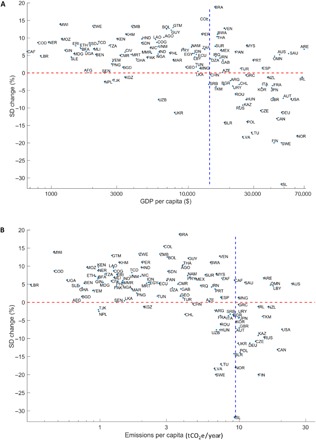
“changes in SD, with decreases outside the tropics but increases over the tropical regions, and relatively higher increases over Amazon Basin (AMZ), Western Africa (WAF), Eastern Africa (EAF), and Southeastern Asia (SEA), consist with previous finding (Bathiany et al., 2018).”
ResultSun, B., Williams, C. M., Li, T., Speakman, J. R., Jin, Z., Lu, H., Luo, L.-G., & Du, W. (2022) · Ecological Monographs · doi:10.1002/ecm.1512 · Cited by 76
Resilience of tropical tree cover: The roles of climate, fire, and herbivory
Staal, A., van Nes, E. H., Hantson, S., Holmgren, M., Dekker, S. C., Pueyo, S., Xu, C., & Scheffer, M. (2018) · Global Change Biology · doi:10.1111/gcb.14408 · Cited by 71
Self-citationLiu, Y., Zhang, H., Zhang, Y., Liang, C., & An, Q. (2022) · Composites Part B Engineering · doi:10.1016/j.compositesb.2022.109988 · Cited by 67
Sikora, R. A., Helder, J., Molendijk, L. P. G., Desaeger, J., den Akker, S. E., & Mahlein, A. (2023) · Annual Review of Phytopathology · doi:10.1146/annurev-phyto-021622-113058 · Cited by 66
Trends of temperature variability: Which variability and what health implications?
Guo, F., Do, V., Cooper, R., Huang, Y., Zhang, P., Ran, J., Zhang, Q., Tian, L., & Fu, Z. (2021) · The Science of The Total Environment · doi:10.1016/j.scitotenv.2020.144487 · Cited by 66
Footprint of greenhouse forcing in daily temperature variability
Kotz, M., Wenz, L., & Levermann, A. (2021) · Proceedings of the National Academy of Sciences · doi:10.1073/pnas.2103294118 · Cited by 63
Impacts of heatwaves on electricity reliability: Evidence from power outage data in China
Liang, J. L., Qiu, Y. L., Wang, B., Shen, X., & Liu, S. (2025) · iScience · doi:10.1016/j.isci.2025.111855 · Cited by 66
“56,57 The magnitudes of these changes align with existing research, which suggests energy demand could increase by approximately 20% under moderate global warming and 25%–58% under severe warming.”
Rapid flips between warm and cold extremes in a warming world
Wu, S., Luo, M., Lau, G. N., Zhang, W., Wang, L., Liu, Z., Lin, L., Wang, Y., Ge, E., Li, J., et al. (2025) · Nature Communications · doi:10.1038/s41467-025-58544-5 · Cited by 92
“28 – 29 and Fig.”
InfluentialPereira, J. C., & Viola, E. (2020) · Journal of Latin American Studies · doi:10.1017/s0022216x20000577 · Cited by 62
Toward sustainable climate change adaptation
Yang, Y., Liu, B., Wang, P., Chen, W., & Smith, T. M. (2020) · Journal of Industrial Ecology · doi:10.1111/jiec.12984 · Cited by 66
Lay, C. R., Sarofim, M. C., Vodonos, A., Mills, D., Jones, R., Schwartz, J. D., & Kinney, P. L. (2021) · The Lancet Planetary Health · doi:10.1016/s2542-5196(21)00058-9 · Cited by 63
Landholm, D. M., Pradhan, P., Wegmann, P., Sanchez, M. A. R., Suárez, J. C., & Kropp, J. P. (2019) · Environmental Research Letters · doi:10.1088/1748-9326/ab3db6 · Cited by 64
Temperature variability and long-run economic development
Linsenmeier, M. (2023) · Journal of Environmental Economics and Management · doi:10.1016/j.jeem.2023.102840 · Cited by 60
“Together with projections of climate models (Bathiany et al., 2018), the results suggest that future changes to interannual temperature variability also tend to increase the costs of climate change in relatively warm (and currently poor) countries.”
BackgroundInfluentialCowan, D. A., Lebre, P. H., Amon, C., Becker, R., Boga, H., Boulangé, A. F., Chiyaka, T., Coetzee, T., de Jager, P., Dikinya, O., et al. (2022) · Microbiome · doi:10.1186/s40168-022-01297-w · Cited by 68
Variability of surface climate in simulations of past and future
Rehfeld, K., Hébert, R., Lora, J. M., Löfverström, M., & Brierley, C. (2020) · Earth System Dynamics · doi:10.5194/esd-11-447-2020 · Cited by 60
Extreme temperatures compromise male and female fertility in a large desert bird
Schou, M. F., Bonato, M., Engelbrecht, A., Brand, Z., SVENSSON, E. I., Melgar, J., Muvhali, P. T., Cloete, S. W. P., & Cornwallis, C. K. (2021) · Nature Communications · doi:10.1038/s41467-021-20937-7 · Cited by 58
North‐West Europe Hottest Days Are Warming Twice as Fast as Mean Summer Days
Patterson, M. (2023) · Geophysical Research Letters · doi:10.1029/2023gl102757 · Cited by 60
“…6 JAN 2023 Accepted 27 APR 2023 1 of 10 Geophysical Research Letters PATTERSON 10.1029/2023GL102757 2 of 10 temperature variability (Bathiany et al., 2018; Fischer & Schär, 2008; Fischer et al., 2007, 2012; Giorgi et al., 2004) which has been explained through positive…”
BackgroundInfluentialXiang, B., Xu, P., Li, R., & Zhang, R. (2024) · ACS Sustainable Chemistry & Engineering · doi:10.1021/acssuschemeng.3c05583 · Cited by 57
Ma, C., Yang, J., Nakayama, S. F., & Honda, Y. (2019) · Environment International · doi:10.1016/j.envint.2019.03.025 · Cited by 60
Modeling plant diseases under climate change: evolutionary perspectives
Yang, L., Ren, M., & Zhan, J. (2022) · Trends in Plant Science · doi:10.1016/j.tplants.2022.12.011 · Cited by 61
Bumann, S. (2021) · Review of Economics · doi:10.1515/roe-2021-0046 · Cited by 55
Climate policy uncertainty and urban green total factor productivity: Evidence from China
Dai, Z., & Zhu, H. (2024) · International Review of Financial Analysis · doi:10.1016/j.irfa.2024.103593 · Cited by 57
Quantifying the role of variability in future intensification of heat extremes
Simolo, C., & Corti, S. (2022) · Nature Communications · doi:10.1038/s41467-022-35571-0 · Cited by 58
“For example, TXsd increase in northern and eastern Europe may be partly explained by a regional strengthening of the meridional gradient, due to the faster background warming ofthe Mediterranean zone 35,36,39,41 .”
InfluentialInégalités mondiales et changement climatique
Guivarch, C., & Taconet, N. (2020) · Revue de l'OFCE/La Revue de l'OFCE · doi:10.3917/reof.165.0035 · Cited by 70
Segnon, A. C., Totin, E., Zougmoré, R. B., Lokossou, J. C., Thompson-Hall, M., Ofori, B. D., Achigan-Dako, E. G., & Gordon, C. (2020) · Climate and Development · doi:10.1080/17565529.2020.1855097 · Cited by 58
“These areas are not only climate change exposure hotspots (Bathiany et al., 2018; de Sherbinin, 2014; Turco et al., 2015), but also hotspots of climate change impacts because of the unique biological, environmental and socio-economic attributes of the region (de Sherbinin, 2014; Diffenbaugh &…”
BackgroundBatıbeniz, F., Hauser, M., & Seneviratne, S. I. (2023) · Earth System Dynamics · doi:10.5194/esd-14-485-2023 · Cited by 58
da Silveira, I. H., Hartwig, S. V., Moura, M. D. N., Cortes, T. R., Junger, W. L., Cirino, G. G., Ignotti, E., & de Oliveira, B. F. A. (2023) · International Journal of Hygiene and Environmental Health · doi:10.1016/j.ijheh.2022.114109 · Cited by 65
Measuring “Weather Whiplash” Events in North America: A New Large‐Scale Regime Approach
Francis, J. A., Skific, N., Vavrus, S., & Cohen, J. L. (2022) · Journal of Geophysical Research Atmospheres · doi:10.1029/2022jd036717 · Cited by 51
Accelerated Historical and Future Warming in the Middle East and North Africa
Malik, A., Stenchikov, G. L., Mostamandi, S., Parajuli, S., Lelieveld, J., Zittis, G., Ahsan, M. S., Atique, L., & Usman, M. (2024) · Journal of Geophysical Research Atmospheres · doi:10.1029/2024jd041625 · Cited by 51
“Desert areas have also warmed at rates exceeding the global average warming rate (Zittis et al., 2022), especially in the tropics and subtropics (Bathiany et al., 2018; Battisti & Naylor, 2009; Fischer & Knutti, 2013; Mora et al., 2017; Vargas Zeppetello et al., 2022; Willett & Sherwood, 2012).”
Syahid, L. N., Sakti, A. D., Virtriana, R., Wikantika, K., Windupranata, W., Tsuyuki, S., Caraka, R. E., & Pribadi, R. (2020) · Remote Sensing · doi:10.3390/rs12223734 · Cited by 49
Diapause and bet‐hedging strategies in insects: a meta‐analysis of reaction norm shapes
Joschinski, J., & Bonte, D. (2021) · Oikos · doi:10.1111/oik.08116 · Cited by 51
Fernández-Alías, A., Marcos, C., Quispe-Becerra, J. I., Sabah, S., & Pérez‐Ruzafa, Á. (2020) · Estuarine Coastal and Shelf Science · doi:10.1016/j.ecss.2020.106901 · Cited by 51
Liu, S. Q., Wang, Y., Zhang, G. J., Wei, L., Wang, B., & Yu, L. (2022) · Nature Communications · doi:10.1038/s41467-022-30145-6 · Cited by 51
The geographic disparity of historical greenhouse emissions and projected climate change
Houtan, K. S. V., Tanaka, K. R., Gagné, T. O., & Becker, S. L. (2021) · Science Advances · doi:10.1126/sciadv.abe4342 · Cited by 47
Bernacchi, C. J., Ruiz‐Vera, U. M., Siebers, M. H., DeLucia, N. J., & Ort, D. R. (2023) · Biochemical Journal · doi:10.1042/bcj20220433 · Cited by 47
Metadata
- Authors
- Bathiany, S., Dakos, V., Scheffer, M., & Lenton, T. M.
- Affiliations
- Wageningen University & Research (NL)
- Centre National de la Recherche Scientifique (FR)
- University of Exeter (GB)
- Corresponding author
- Bathiany, Sebastian
- Venue
- Science Advances
- Published
- 2018-05-04
- Volume
- 4
- Issue
- 5
- Pages
- eaar5809-eaar5809
- ISSN
- 2375-2548 (ISSN-L)
- PMC
- PMC5931768
- OpenAlex
- W2799499225
- Cited by
- 479
- References
- 56
- Citations by year
- 2026: 26 · 2025: 64 · 2024: 72 · 2023: 64 · 2022: 80 · 2021: 63 · 2020: 55 · 2019: 44 · 2018: 11
- FWCI
- 25.35
- Type
- journal article
- Language
- en
- Open access
- gold
- doi.org
- Licence
- cc-by-nc
- Locations
- Science Advances (publishedVersion, cc-by-nc)
- Europe PMC (PubMed Central) (publishedVersion, cc-by-nc)
- PubMed Central (publishedVersion, cc-by-nc)
- PubMed (publishedVersion)
- Socio-Environmental Systems Modeling (acceptedVersion, cc-by-nc)
- HAL (submittedVersion, cc-by-nc)
- Figshare (submittedVersion, cc-by-nc)
- Open Research Exeter (University of Exeter) (submittedVersion, cc-by-nc)
- Data Archiving and Networked Services (DANS) (submittedVersion, cc-by-nc)
- Funders
- Netherlands Organisation for Scientific Research (Zwaartekracht project NESSC)
- Topics
- Physical Sciences › Environmental Science › Global and Planetary Change › Climate variability and models
- Physical Sciences › Environmental Science › Global and Planetary Change › Climate Change and Environmental Impact
- Life Sciences › Agricultural and Biological Sciences › Agronomy and Crop Science › Climate change impacts on agriculture
- Keywords
- temperature variability, climate change projections, climate models, developing countries, climate inequality, Sahel, India, Southeast Asia, soil drying, atmospheric structure, meridional temperature gradient, sea ice decline, extreme weather events, climate change vulnerability
About these checks
Registry, retraction, Cites and statistics results are computed, not judged, with one exception: a printed reference that no index lists is read once by a model before it counts as a citation error. Claims are extracted by a model and kept only when their quote appears verbatim in the text; each cited source is then checked, with a model’s help, for whether it says what the claim relies on. Those verdicts can be wrong — read the claim’s quote and the cited source before relying on one.
Statistics and arithmetic are recomputed, not judged.
Confidence bands are shown only for fields calibrated on our annotated test set. None is calibrated yet, so no band is shown.
What counts as a claim ›How we measure confidence ›How we check this ›
Are you an author, or do you see a problem with this page? Request a review
Data sources
Bibliographic data: Semantic Scholar, OpenAlex, Crossref.
Contains information from the Semantic Scholar Academic Graph Datasets, made available under the ODC Attribution License (ODC-BY 1.0).
Semantic Scholar’s data is described in: Kinney, R., et al. (2023). The Semantic Scholar Open Data Platform. arXiv:2301.10140.
