

The DOI matches its Crossref record, with a small difference in title or year; 103 of the 104 references it cites were found in a registry or an index.
Martinize2 and Vermouth provide a unified framework for molecular topology generation
Open accessPublished version of a preprint
Abstract
Ongoing advances in force field and computer hardware development enable the use of molecular dynamics (MD) to simulate increasingly complex systems with the ultimate goal of reaching cellular complexity. At the same time, rational design by high-throughput (HT) simulations is another forefront of MD. In these areas, the Martini coarse-grained force field, especially the latest version (i.e. v3), is being actively explored because it offers an enhanced spatial-temporal resolution. However, the automation tools for preparing simulations with the Martini force field, accompanying the previous version, were not designed for HT simulations or studies of complex cellular systems. Therefore, they become a major limiting factor. To address these shortcomings, we present the open-source Vermouth python library. Vermouth is designed to become the unified framework for developing programs, which prepare, run, and analyze Martini simulations of complex systems. To demonstrate the power of the Vermouth library, the Martinize2 program is showcased as a generalization of the martinize script, originally aimed to set up simulations of proteins. In contrast to the previous version, Martinize2 automatically handles protonation states in proteins and post-translation modifications, offers more options to fine-tune structural biases such as the elastic network (EN), and can convert non-protein molecules such as ligands. Finally, Martinize2 is used in two high-complexity benchmarks. The entire I-TASSER protein template database as well as a subset of 200,000 structures from the AlphaFold Protein Structure Database are converted to CG resolution and we illustrate how the checks on input structure quality can safeguard HT applications.
Overview
The claims and statistics of this paper haven’t been checked yet.
Run the check — free, no account needed. It reads the open-access text and checks the sources it cites.
Integrity signals
Registry
Cites
Statistics
Figures
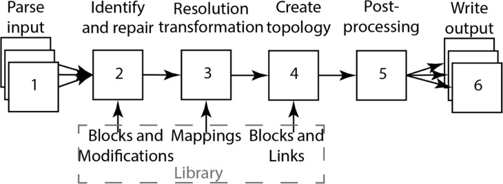
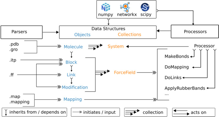
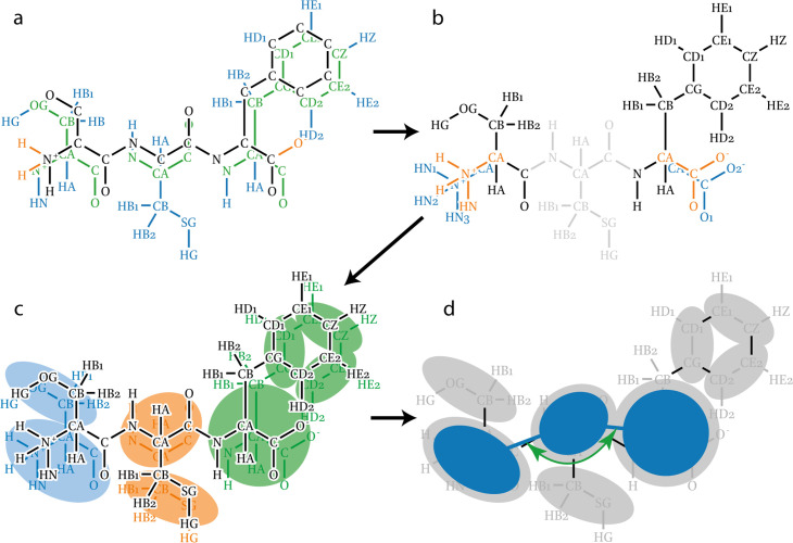
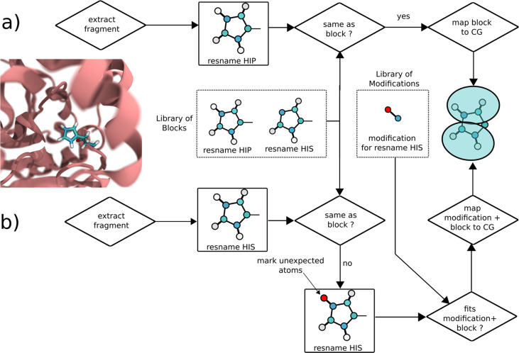
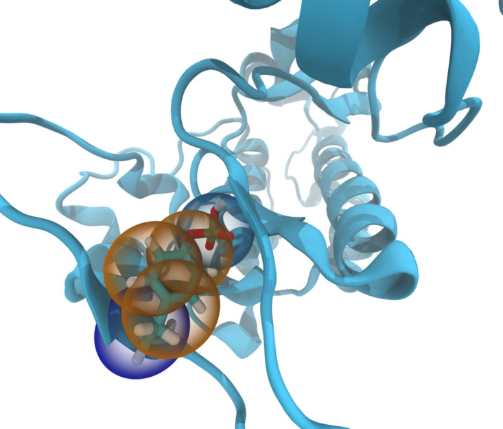
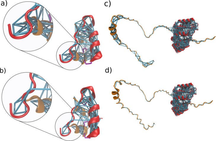
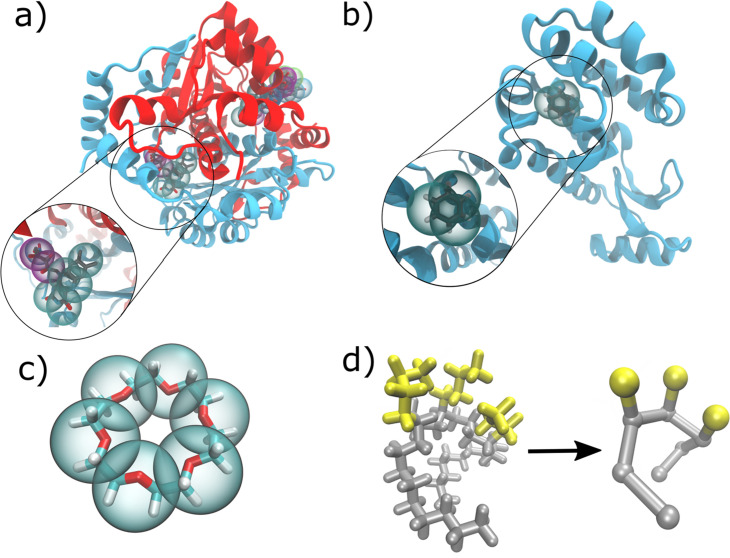
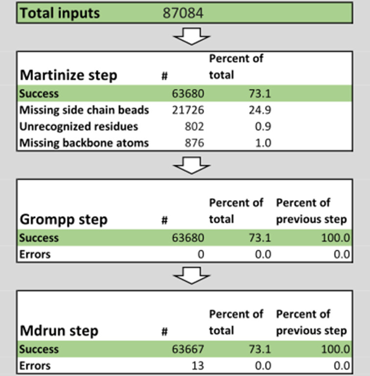
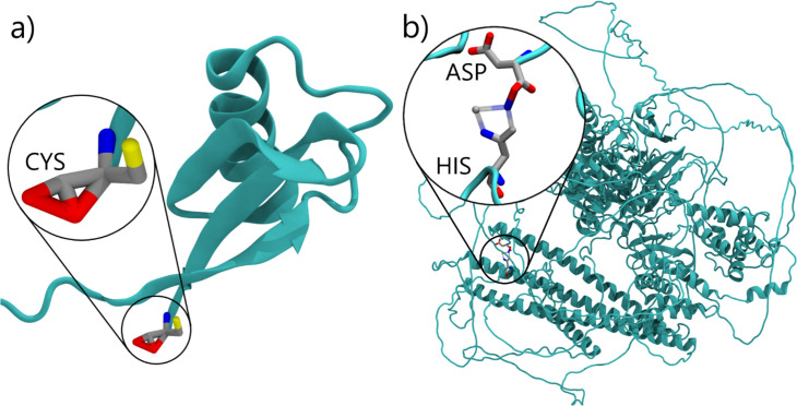
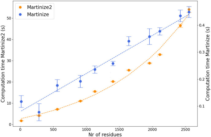
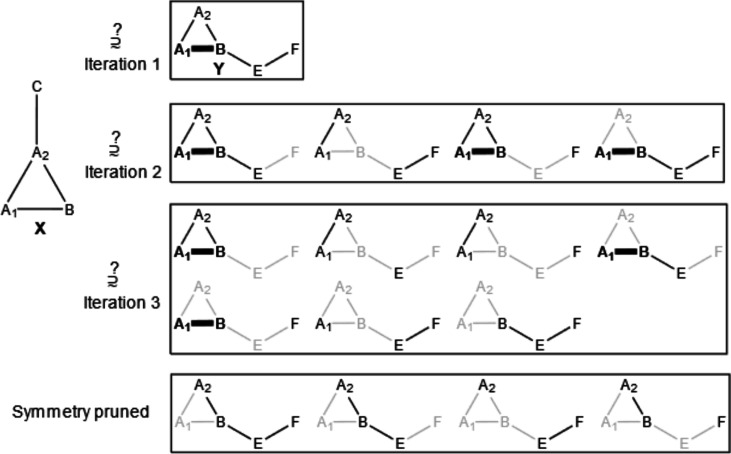
Verification
Claims the paper makes
The claims and statistics of this paper haven’t been checked yet.
Run the check — free, no account needed. It reads the open-access text and checks the sources it cites.
Self-check
Percentages, sums and reported differences re-computed from the paper’s own numbers.
The self-check needs the paper’s full text.
Citations
Cites
Highly accurate protein structure prediction with AlphaFold
Jumper, J., Evans, R., Pritzel, A., Green, T., Figurnov, M., Ronneberger, O., Tunyasuvunakool, K., Bates, R., Žídek, A., Potapenko, A., et al. (2021) · Nature · doi:10.1038/s41586-021-03819-2 · Cited by 43,764
SciPy 1.0: fundamental algorithms for scientific computing in Python
Virtanen, P., Gommers, R., Oliphant, T. E., Haberland, M., Reddy, T., Cournapeau, D., Burovski, E., Peterson, P., Weckesser, W., Bright, J., et al. (2020) · Nature Methods · doi:10.1038/s41592-019-0686-2 · Cited by 38,430
Molecular dynamics with coupling to an external bath
Berendsen, H. J. C., Postma, J. P. M., van Gunsteren, W. F., DiNola, A., & Haak, J. R. (1984) · The Journal of Chemical Physics · doi:10.1063/1.448118 · Cited by 31,057
Abraham, M. J., Murtola, T., Schulz, R., Páll, S., Smith, J. C., Hess, B., & Lindahl, E. (2015) · SoftwareX · doi:10.1016/j.softx.2015.06.001 · Cited by 27,190
Harris, C. R., Millman, K. J., van der Walt, S. J., Gommers, R., Virtanen, P., Cournapeau, D., Wieser, E., Taylor, J., Berg, S., Smith, N. J., et al. (2020) · Nature · doi:10.1038/s41586-020-2649-2 · Cited by 23,826 · cited 1×
“In addition, the library relies on only three permissibly licensed open-software projects, namely numpy ( Harris et al., 2020 ), scipy ( Virtanen et al., 2020 ), and networkx ( Hagberg et al., 2008 ).”
Polymorphic transitions in single crystals: A new molecular dynamics method
Parrinello, M., & Rahman, A. (1981) · Journal of Applied Physics · doi:10.1063/1.328693 · Cited by 20,009
The FAIR Guiding Principles for scientific data management and stewardship
Wilkinson, M. D., Dumontier, M., Aalbersberg, I. J., Appleton, G., Axton, M., Baak, A., Blomberg, N., Boiten, J.-W., da Silva Santos, L. B., Bourne, P. E., et al. (2016) · Scientific Data · doi:10.1038/sdata.2016.18 · Cited by 18,423 · cited 2×
“( Chue Hong et al., 2022 ; Wilkinson et al., 2016 ; Alibay et al., 2022 ) The FAIR principles Wilkinson et al., 2016 , originally designed to improve data management and reproducibility in science, have recently been extended to research software in a more general sense.”
Canonical sampling through velocity rescaling
Bussi, G., Donadio, D., & Parrinello, M. (2007) · The Journal of Chemical Physics · doi:10.1063/1.2408420 · Cited by 18,327
Scalable molecular dynamics with NAMD
Phillips, J. C., Braun, R., Wang, W., Gumbart, J., Tajkhorshid, E., Villa, E., Chipot, C., Skeel, R. D., Kalé, L., & Schulten, K. (2005) · Journal of Computational Chemistry · doi:10.1002/jcc.20289 · Cited by 16,914
Kabsch, W., & Sander, C. (1983) · Biopolymers · doi:10.1002/bip.360221211 · Cited by 15,320
Research works printed but not linked: 3
- Chung, 2010, Graph theory in the information age, Notices of the American Mathematical Society, 57, 726
- Kroon PC, Barnoud J, Brasnett C, Grunewald F, Peter M, Tadema M, Liu X, Araújo LB, marrink-lab, Tsjerk, Romumrn. 2025. Vermouth-martinize. Software Heritage. swh:1:rev:a3037bc2544daa0faa8ba105b9670a2659885d43. https://archive.softwareheritage.org/swh:1:dir:270aae9780a9b8f07c0c1411175f4e982bc0b539;origin=https://github.com/marrink-lab/vermouth-martinize;visit=swh:1:snp:155374469e37d66bb87fc5832a0e0f314e27ca85;anchor=swh:1:rev:a3037bc2544daa0faa8ba105b9670a2659885d43.
- marrink-lab. 2025. Martinize-examples. Software Heritage. swh:1:rev:78a81b00ff8bc9798386c442251a14f568e8f8eb. https://archive.softwareheritage.org/swh:1:dir:0869dc8a9197f72f91847dbb5739f97fb20576bd;origin=https://github.com/marrink-lab/martinize-examples;visit=swh:1:snp:85479e72dfea864eca7b37f1eb7390153820e6eb;anchor=swh:1:rev:78a81b00ff8bc9798386c442251a14f568e8f8eb.
Cited by
Sorted by citations
Martini 3 Coarse-Grained Force Field for Cholesterol
Borges-Araújo, L., Borges-Araújo, A. C., Öztürk, T. N., Ramirez-Echemendía, D. P., Fábián, B., Carpenter, T. S., Thallmair, S., Barnoud, J., Ingólfsson, H. I., Hummer, G., et al. (2023) · Journal of Chemical Theory and Computation · doi:10.1021/acs.jctc.3c00547 · Cited by 87
Self-citationMartini3-IDP: improved Martini 3 force field for disordered proteins
Wang, L., Brasnett, C., Borges-Araújo, L., Souza, P. C. T., & Marrink, . J. (2025) · Nature Communications · doi:10.1038/s41467-025-58199-2 · Cited by 70
Self-citationFacilitating CG Simulations with MAD: The MArtini Database Server
Hilpert, C., Beranger, L., Souza, P. C. T., Vainikka, P. A., Nieto, V., Marrink, S. J., Monticelli, L., & Launay, G. (2023) · Journal of Chemical Information and Modeling · doi:10.1021/acs.jcim.2c01375 · Cited by 51
Self-citationAccurate model and ensemble refinement using cryo-electron microscopy maps and Bayesian inference
Hoff, S., Thomasen, F. E., Lindorff‐Larsen, K., & Bonomi, M. (2024) · PLoS Computational Biology · doi:10.1371/journal.pcbi.1012180 · Cited by 43
Hexokinase-I directly binds to a charged membrane-buried glutamate of mitochondrial VDAC1 and VDAC2
Bieker, S., Timme, M., Woge, N., Hassan, D., Brown, C. M., Marrink, . J., Melo, M. N., & Holthuis, J. C. M. (2025) · Communications Biology · doi:10.1038/s42003-025-07551-9 · Cited by 30
Mehta, N., Mondal, S., Watson, E. T., Cui, Q., & Chapman, E. R. (2024) · Nature Communications · doi:10.1038/s41467-023-44414-5 · Cited by 28
Cryo-EM architecture of a near-native stretch-sensitive membrane microdomain
Kefauver, J. M., Hakala, M., Zou, X., Alba, J., Espadas, J., Tettamanti, M. G., Gajić, J., Gabus, C., Campomanes, P., Estrozi, L. F., et al. (2024) · Nature · doi:10.1038/s41586-024-07720-6 · Cited by 27
Multiphasic condensates formed with mono-component of tetrapeptides via phase separation
Zhou, L., Zhu, L., Wang, C., Xu, T., Wang, J., Zhang, B., Zhang, X., & Wang, H. (2025) · Nature Communications · doi:10.1038/s41467-025-58060-6 · Cited by 31
CLCC1 promotes hepatic neutral lipid flux and nuclear pore complex assembly
Mathiowetz, A. J., Meymand, E. S., Parlakgül, G., van Hilten, N., Torres, E. F., Artico, L. L., Deol, K. K., Lange, M., Pang, S. P., Doubravsky, C. E., et al. (2026) · Nature · doi:10.1038/s41586-025-10064-4 · Cited by 26
Prediction of Small-Molecule Partitioning into Biomolecular Condensates from Simulation
Emelianova, A., Garcia, P. L., Tan, D., & Joseph, J. A. (2025) · JACS Au · doi:10.1021/jacsau.5c00291 · Cited by 23
Sequence and structural determinants of RNAPII CTD phase-separation and phosphorylation by CDK7
Linhartova, K., Falginella, F. L., Mátl, M., Šebesta, M., Vácha, R., & Štefl, R. (2024) · Nature Communications · doi:10.1038/s41467-024-53305-2 · Cited by 22
Park, P., Matsubara, D. K., Barzotto, D. R., Lima, F. S., Chaimovich, H., Marrink, . J., & Cuccovia, I. M. (2024) · Scientific Reports · doi:10.1038/s41598-024-60601-w · Cited by 21
Soni, J., Gupta, S., & Mandal, T. (2024) · Journal of Chemical Theory and Computation · doi:10.1021/acs.jctc.4c00645 · Cited by 19
Bartocci, A., Grazzi, A., Awad, N., Corringer, P., Souza, P. C. T., & Cecchini, M. (2024) · Nature Communications · doi:10.1038/s41467-024-53098-4 · Cited by 17
Self-citationNonspecific Yet Selective Interactions Contribute to Small Molecule Condensate Binding
Wang, C., Kilgore, H. R., Latham, A. P., & Zhang, B. (2024) · Journal of Chemical Theory and Computation · doi:10.1021/acs.jctc.4c01024 · Cited by 16
Martini 3 Force Field Parameters for Protein Lipidation Post-Translational Modifications
Koukos, P. I., Dehghani‐Ghahnaviyeh, S., Velez‐Vega, C., Manchester, J. I., Tieleman, D. P., Duca, J. S., Souza, P. C. T., & Cournia, Z. (2023) · Journal of Chemical Theory and Computation · doi:10.1021/acs.jctc.3c00604 · Cited by 16
Self-citationYu, Y., Liu, Q., Zeng, J., Tan, Y., Tang, Y., & Wei, G. (2024) · Chemical Science · doi:10.1039/d4sc03645j · Cited by 14
MartiniGlass: a Tool for Enabling Visualization of Coarse-Grained Martini Topologies
Brasnett, C., & Marrink, . J. (2025) · Journal of Chemical Information and Modeling · doi:10.1021/acs.jcim.4c02277 · Cited by 17
Self-citationMartini on the Rocks: Can a Coarse-Grained Force Field Model Crystals?
Hosseini, A., & van der Spoel, D. (2024) · The Journal of Physical Chemistry Letters · doi:10.1021/acs.jpclett.4c00012 · Cited by 12
Yue, Y., Li, S., Cheng, Y., Wang, L., Hou, T., Zhu, Z., & He, S. (2024) · Nature Communications · doi:10.1038/s41467-024-53583-w · Cited by 12
UBE2J2 sensitizes the ERAD ubiquitination cascade to changes in membrane lipid saturation
Vrentzou, A., Leidner, F., Schmidt, C. C., Grubmüller, H., & Stein, A. (2025) · Nature Communications · doi:10.1038/s41467-025-64777-1 · Cited by 9
Fast Parametrization of Martini3 Models for Fragments and Small Molecules
Szczuka, M., Pereira, G. P., Walter, L. J., Guéroult, M., Poulain, P., Bereau, T., Souza, P. C. T., & Chavent, M. G. (2025) · Journal of Chemical Theory and Computation · doi:10.1021/acs.jctc.5c01178 · Cited by 9
Self-citationNemchinova, M., Schuurman‐Wolters, G. K., Whittaker, J. J., Arkhipova, V., Marrink, . J., Poolman, B., & Guskov, A. (2024) · The Journal of Physical Chemistry B · doi:10.1021/acs.jpcb.4c02662 · Cited by 9
Folded domains impose structural heterogeneity and attenuated dynamics in biomolecular condensates
Wang, L., & Marrink, . J. (2026) · Nature Communications · doi:10.1038/s41467-026-71778-1 · Cited by 8
van Tilburg, M., Marrink, . J., König, M., & Grünewald, F. (2023) · Journal of Chemical Theory and Computation · doi:10.1021/acs.jctc.3c00961 · Cited by 8
Self-citationMondal, S., Mangiarotti, A., Dimova, R., & Cui, Q. (2025) · Communications Chemistry · doi:10.1038/s42004-025-01810-w · Cited by 7
Cullen, M., Biancaniello, C., Taškova, K., Miletić, V., Mercadante, D., & Simone, A. D. (2026) · Journal of the American Chemical Society · doi:10.1021/jacs.5c22987 · Cited by 7
Roessner, R. A., Floquet, N., & Louet, M. (2025) · Journal of Chemical Information and Modeling · doi:10.1021/acs.jcim.5c00202 · Cited by 8
Osorio-Méndez, J. F., Pardo-Rodriguez, D., Rocha‐Roa, C., Toro, L. J., Muñoz-Tabares, L., Recalde-Reyes, D. P., & Cala, M. P. (2025) · Parasites & Vectors · doi:10.1186/s13071-025-06861-5 · Cited by 6
Zhao, M., Lopes, L. J. S., Sahni, H., Yadav, A., Do, H. N., Reddy, T. J., López, C. A., Neale, C., & Gnanakaran, S. (2024) · The Journal of Physical Chemistry B · doi:10.1021/acs.jpcb.4c05018 · Cited by 6
Compartment‐guided assembly of large‐scale molecular models with Bentopy
Westendorp, M. S. S., Stevens, J. A., Brown, C. M., Dommer, A. C., Wassenaar, T. A., Bruininks, B. M. H., & Marrink, . J. (2026) · Protein Science · doi:10.1002/pro.70480 · Cited by 7
Self-citationNiemelä, A., & Koivuniemi, A. (2024) · PLoS Computational Biology · doi:10.1371/journal.pcbi.1012137 · Cited by 5
Hedger, G., & Yen, H. (2025) · Journal of Molecular Biology · doi:10.1016/j.jmb.2025.168937 · Cited by 6
Optimized Protein–Excipient Interactions in the Martini 3 Force Field
Prass, T. M., Lindorff‐Larsen, K., Garidel, P., Blech, M., & Schäfer, L. V. (2025) · Journal of Chemical Information and Modeling · doi:10.1021/acs.jcim.4c02338 · Cited by 5
Jiang, Y., & Ha‐Duong, T. (2025) · Journal of Chemical Theory and Computation · doi:10.1021/acs.jctc.5c00212 · Cited by 6
Mechanistic studies of mycobacterial glycolipid biosynthesis by the mannosyltransferase PimE
Liu, Y., Brown, C. M., Borges, N., Nobre, R. N., Erramilli, S. K., Dufrisne, M. B., Kloss, B., Giacometti, S. I., Esteves, A. M., Timóteo, C. G., et al. (2025) · Nature Communications · doi:10.1038/s41467-025-57843-1 · Cited by 5
Sharma, A., Maurya, S., Tripathi, T., & Padhi, A. K. (2024) · Acta Tropica · doi:10.1016/j.actatropica.2024.107444 · Cited by 5
Delineating the shape of COat Protein complex-II coated membrane bud
Paul, S., Audhya, A., & Cui, Q. (2024) · bioRxiv · doi:10.1093/pnasnexus/pgae305 · Cited by 5
Oqua, A. I., Chao, K., Eid, L. E., Casteller, L., Miguéns, A., Barg, S., Jones, B. J., de la Serna, J. B., Rouse, S. L., & Tomás, A. (2024) · eLife · doi:10.7554/elife.101011.1 · Cited by 4
CCD2MD: A Suite of Packages for Preparing Co-Folded Outputs for Molecular Dynamics Simulations
Blow, K. E., Parrag, M., & Stansfeld, P. J. (2025) · Journal of Chemical Information and Modeling · doi:10.1021/acs.jcim.5c02066 · Cited by 3
TMEM170 proteins are lipid scramblases associated with bridge-type lipid transporters BLTP1/Csf1
Rocha‐Roa, C., Blair, P. C., Sidhu, G., Álvarez, D., Davey, M., Conibear, E., & Vanni, S. (2025) · Nature Structural & Molecular Biology · doi:10.1038/s41594-025-01716-0 · Cited by 5
Linnik, D., Sultanji, S., Stevens, J. A., Schuurman‐Wolters, G. K., de Boer, R., Punter, C. M., Marrink, . J., Maslov, I., & Poolman, B. (2026) · Nature Communications · doi:10.1038/s41467-026-69951-7 · Cited by 3
Structural basis of signal peptide recognition by the signal peptidase complex
Liaci, A. M., Vismpas, D., Kjølbye, L. R., Skalidis, I., Pereira, G. P., Koh, F., Gröllers‐Mulderij, M., Kotecha, A., Souza, P. C. T., & Förster, F. G. (2026) · Nature Communications · doi:10.1038/s41467-026-73423-3 · Cited by 3
Self-citationBigting, K. V., Nag, S., & An, Y. (2026) · Journal of Chemical Information and Modeling · doi:10.1021/acs.jcim.5c02903 · Cited by 3
Costafrolaz, J., Degeorges, L., Panis, G., Vallet, S.-U., Gomariz, M. V., Meireles, F. T. P., Peraro, M. D., Fröhlich, K. S., & Viollier, P. H. (2026) · The EMBO Journal · doi:10.1038/s44318-025-00668-x · Cited by 3
Sarter, T., Karavalasi, A., & Friess, W. (2026) · Molecular Pharmaceutics · doi:10.1021/acs.molpharmaceut.5c01525 · Cited by 2
Li, J., Guo, H., & Song, C. (2026) · Journal of Chemical Theory and Computation · doi:10.1021/acs.jctc.5c01859 · Cited by 2
The molecular basis of mitochondrial crista formation by the MIC10 complex
Brown, C. M., Wassenaar, T. A., Freyberg, Z., & Marrink, . J. (2026) · Science Advances · doi:10.1126/sciadv.aee8657 · Cited by 2
Self-citationMicroscopically segregated ligand distribution in co-assembled peptide-amphiphile nanofibers
Pial, T. H., Li, Y., & de la Cruz, M. O. (2024) · Soft Matter · doi:10.1039/d4sm00315b · Cited by 2
Coarse-grained modeling of annexin A2-induced microdomain formation on a vesicle
Lindsay, S., & Li, Y. (2024) · Biophysical Journal · doi:10.1016/j.bpj.2024.06.006 · Cited by 2
Hooten, M., Murthy, N. S., Pal, N., Khare, S. D., Gormley, A. J., & Dutt, M. (2025) · The Journal of Chemical Physics · doi:10.1063/5.0247634 · Cited by 2
A Charge-Driven Strategy for Covalent Modification and Modulation of Biomolecular Condensates
Chen, Z., Liu, L., Cattin, J., Knowles, T. P. J., & Bernardes, G. J. L. (2025) · Journal of the American Chemical Society · doi:10.1021/jacs.5c06625 · Cited by 2
SND3 is the membrane insertase within a fungal multipass transloconPreprint
Yang, T.-J., Mukherjee, S., Langer, J. D., Hummer, G., & McDowell, M. A. (2025) · bioRxiv · doi:10.1101/2025.07.08.663624 · Cited by 2
Efficient Protein–Ligand Binding Free Energy Estimation with Coarse-Grained Funnel Metadynamics
Grazzi, A., Brown, C. M., Sironi, M., Marrink, . J., & Pieraccini, S. (2026) · Journal of Chemical Theory and Computation · doi:10.1021/acs.jctc.5c01785 · Cited by 1
Li, F., Radhakrishnan, A., Gautam, S., Diaz, G., Sundaram, R. V. K., Coleman, J., Zheng, H., Grushin, K. S., Chavent, M. G., Rothman, J. E., et al. (2026) · Proceedings of the National Academy of Sciences · doi:10.1073/pnas.2523347123 · Cited by 1
Ancestral neuronal receptors are bacterial accessory toxins
Raoelijaona, F., Szczepaniak, J., Schahl, A., Bray, J. E., Zhou, J. C., Baker, L. A., Omari, K. E., Lowe, E. D., Low, Y. S., Rodriguez, C., et al. (2026) · Nature Communications · doi:10.1038/s41467-026-69246-x · Cited by 1
Comparing multislice projections of MD simulations with cryo-EM exposes structural prediction errors
Mohammed, A., Lincoff, J., Natale, A. M., Ophus, C., Grabe, M., Frost, A., & Moss, F. R. (2026) · Biophysical Journal · doi:10.1016/j.bpj.2026.02.016 · Cited by 1
Improving Conformational Ensembles of Folded Proteins in GoMartini
Kalutskii, M. A., Wilson, C. J., Grubmüller, H., & Igaev, M. (2026) · Journal of Chemical Theory and Computation · doi:10.1021/acs.jctc.5c01816 · Cited by 1
Drajkowska, A., & Molski, A. (2026) · The Journal of Physical Chemistry B · doi:10.1021/acs.jpcb.5c07780 · Cited by 1
Fast-Forward: Automatic Assignment and Assessment of Bonded Parameters for the Martini Force Field
Brasnett, C., Fidlin, M., Duve, T., Thallmair, S., Marrink, . J., & Grünewald, F. (2026) · Journal of Chemical Information and Modeling · doi:10.1021/acs.jcim.6c01107 · Cited by 3
Self-citationCáceres-Quezada, Á., Borroto‐Escuela, D. O., & Fierro, A. (2026) · Journal of Chemical Information and Modeling · doi:10.1021/acs.jcim.6c00308 · Cited by 1
An optimized contact map for GōMartini 3 enabling conformational changes in protein assemblies
Olivos-Ramirez, G. E., Cofas‐Vargas, L. F., Marrink, . J., & Poma, A. B. (2026) · Biophysical Journal · doi:10.1016/j.bpj.2026.04.024 · Cited by 1
Atg18 interaction positions Atg2 for efficient lipid transfer into phagophore elongation
Ramirez, S. C., Shvarev, D., Duarte, P. V., Ahmed, Y., Milach, J., Lang, E., Kuchenbuch, S., Vanni, S., Reggiori, F., Moeller, A., et al. (2026) · The EMBO Journal · doi:10.1038/s44318-026-00802-3 · Cited by 1
MartiniSurf: Automated Simulations of Surface-Immobilized Biomolecular Systems with Martini
Jiménez-García, J. C., López‐Gallego, F., López, X., & Sancho, D. D. (2026) · Journal of Chemical Information and Modeling · doi:10.1021/acs.jcim.6c00953 · Cited by 1
Dehkhoda, F., Chhabra, Y., Whelan, F., Nowell, C. J., Morris, M. J., Furness, S. G. B., & Brooks, A. J. (2026) · The Journal of Immunology · doi:10.1093/jimmun/vkag118 · Cited by 1
Membrane lipid composition and amino acid sequence determine binding of SARS-CoV-2 fusion peptides
Jiménez-Millán, S., Maestro, A., & Sasselli, I. R. (2026) · Journal of Colloid and Interface Science · doi:10.1016/j.jcis.2026.141021 · Cited by 2
Pires, I. S., Gordon, E., Kindopp, A., Stoneman, A. D., Covarrubias, G., Esparza, G. J., Gomerdinger, V. F., Maiorino, L., Suh, H., Irvine, D. J., et al. (2026) · ACS Nano · doi:10.1021/acsnano.6c02817 · Cited by 1
Encounter-State Over-Anchoring Governs Productive PETase Binding on PET Surfaces
Huo, C., Wang, J., & Chu, X. (2026) · Journal of Chemical Theory and Computation · doi:10.1021/acs.jctc.6c00544 · Cited by 1
Amphipathic β-Sheet-Forming Octapeptide Self-Assembly Using the Martini Potential Family
Maity, D., & Qiao, B. (2026) · ACS Omega · doi:10.1021/acsomega.6c02457 · Cited by 1
Kwon, H., & Li, Y. (2026) · Food Hydrocolloids · doi:10.1016/j.foodhyd.2026.113310 · Cited by 1
Presynaptic accumulation of APP-CTFβ may contribute to synaptic dysfunction in Alzheimer’s disease
Kapadia, A., Schuhmann, F., Daşkın, E., Walter, J., Lindahl, I., Rahmani, N., Morrema, T. H. J., Rozemüller, A. J. M., Boon, B. D. C., Pezeshkian, W., et al. (2026) · The EMBO Journal · doi:10.1038/s44318-026-00899-6 · Cited by 1
Duncan, A. L., Gao, Y., Haanappel, E., Im, W., & Chavent, M. G. (2023) · ChemRxiv · doi:10.26434/chemrxiv-2023-mfc5k · Cited by 1
Mondal, S., Mangiarotti, A., Dimova, R., & Cui, Q. (2025) · bioRxiv (Cold Spring Harbor Laboratory) · doi:10.1101/2025.05.16.654554 · Cited by 1
Ceramides disrupt hexokinase HKI-VDAC complex assembly and modulate VDAC tiltingPreprint
Timme, M., Holthuis, J. C. M., & Melo, M. N. (2026) · bioRxiv (Cold Spring Harbor Laboratory) · doi:10.64898/2026.04.25.720789 · Cited by 1
Guillén-Samander, A., Ahmed, Y., Ribeiro-Holbein, A., Cubillán-Marín, J., Höhn, K., Rocha‐Roa, C., Dröge, J., Panitzsch, L. S., Burda, P., Gilberger, T., et al. (2026) · bioRxiv (Cold Spring Harbor Laboratory) · doi:10.64898/2026.09.11.750981 · Cited by 1
Optimising excipient properties to prevent aggregation in biopharmaceutical formulationsPreprint
King, T., Humphrey, J., Laughton, C. A., Thomas, N. R., & Hirst, J. D. (2023) · ChemRxiv · doi:10.26434/chemrxiv-2023-rgvlz
Duncan, A. L., Gao, Y., Haanappel, E., Im, W., & Chavent, M. G. (2024) · Methods in molecular biology · doi:10.1007/978-1-0716-3734-0_19
Sahoo, A. K., & Hanson, S. M. (2024) · bioRxiv (Cold Spring Harbor Laboratory) · doi:10.1101/2024.05.29.596440
Hooten, M., Murthy, S., Pal, N., Khare, S. D., Gormley, A. J., & Dutt, M. (2024) · bioRxiv (Cold Spring Harbor Laboratory) · doi:10.1101/2024.09.22.614383
Carnahan, C. F., He, W., Öztürk, T. N., Wang, Y., Ngassam, V. N., Noy, A., Carpenter, T. S., Voss, J. C., Coleman, M. A., & Parikh, A. N. (2025) · bioRxiv (Cold Spring Harbor Laboratory) · doi:10.1101/2025.04.10.648283
Bifunctional architecture enables substrate catalysis and channeling in Paracoccus TMAO demethylase
Thach, T. T., Dhanabalan, K., Maurya, S., Han-Hallett, Y., Quan, S., Allison, J. R., Ramanathan, G., & Ramaswamy, S. (2026) · eLife · doi:10.7554/elife.109964.4
Muthachikavil, A. V., von Appen, A., & Kühne, T. D. (2025) · Proteins Structure Function and Bioinformatics · doi:10.1002/prot.70105
Mandal, N., Stevens, J. A., Poma, A. B., Surpeta, B., Sequeiros-Borja, C. E., Thirunavukarasu, A. S., Marrink, . J., & Brezovský, J. (2026) · Journal of Chemical Theory and Computation · doi:10.1021/acs.jctc.5c01727
Grazzi, A., Brown, C. M., Sironi, M., Marrink, . J., & Pieraccini, S. (2026) · bioRxiv (Cold Spring Harbor Laboratory) · doi:10.64898/2026.02.24.707696
Hu, Z., Yue, K., Zhong, W., & Zhang, G. (2026) · Polymers · doi:10.3390/polym18070781
Kim, S. H., Park, J. S., Kim, D. Y., Park, Y. E., Kim, H., Kim, S. T., Min, Y.-H., & Park, M. K. (2026) · International Journal of Biological Macromolecules · doi:10.1016/j.ijbiomac.2026.154017
Avila, J., Park, P., Singh, Y., Amaral, P., Castro, I., ten-Caten, F., Schuch, V., Gonçalves, A. N. A., Giddaluru, J., Morais, M. C. C., et al. (2026) · Journal of Medical Virology · doi:10.1002/jmv.70932
Ropón‐Palacios, G., Crespi, L. G. F., Martins, I. B. S., Rocchia, W., & de Araújo, A. S. (2026) · Journal of Chemical Information and Modeling · doi:10.1021/acs.jcim.6c01334
Yang, S., & Song, C. (2026) · bioRxiv (Cold Spring Harbor Laboratory) · doi:10.64898/2026.04.30.721921
Photoreceptor outer segment disk rim curvature relies on a tetraspanin interaction web
Boucher, R. C., Milstein, M. L., Hossein, A., Cavanaugh, B. L., Sodt, A. J., Beaven, A. H., & Goldberg, A. F. X. (2026) · Journal of Biological Chemistry · doi:10.1016/j.jbc.2026.113136
On the Prospect of Chemically Transferable Coarse-Grained Electronic Models for Soft Materials
Kidder, K. M., Kim, S., & Jackson, N. E. (2026) · The Journal of Physical Chemistry B · doi:10.1021/acs.jpcb.6c00843
Wang, L., Zheng, Z., Liao, Z., Zhang, P., Yang, J., Wei, H., Yan, J., Chu, X.-Q., Fan, J., & Liu, W. F. (2026) · Acta Biomaterialia · doi:10.1016/j.actbio.2026.05.019
Full-length SARS-CoV-2 envelope protein adopts an interfacial topology in lipid bilayers
Morris, A. K., Wardrip, L., Sahu, I. D., & Lorigan, G. A. (2026) · Biochimica et Biophysica Acta (BBA) - Biomembranes · doi:10.1016/j.bbamem.2026.184539
Activation of the bridge-like lipid transfer protein Atg2 by Atg1-mediated phosphorylationPreprint
Achleitner, S., Tulli, S., Cabezudo, A. C., Schuschnig, M., Baumann, V., Schmid, M., Hummer, G., & Martens, S. (2026) · bioRxiv (Cold Spring Harbor Laboratory) · doi:10.64898/2026.05.15.725374
Study of line tension and its impact on protein organization in model domain-forming membranes
Gupta, S., & Mandal, T. (2026) · Physical Chemistry Chemical Physics · doi:10.1039/d6cp01175f
TDP-43 self-assembly is regulated by its disordered NLS-regionPreprint
Hutten, S., Pekbilir, E., Bourgeois, B. M. R., Ping, X., Rickert, C., Kuhr, N. S., Knabe, N., Mosna, S., Madl, T., Stelzl, L. S., et al. (2026) · bioRxiv (Cold Spring Harbor Laboratory) · doi:10.64898/2026.06.06.730435
Atomistic simulations reveal sub-µs contact dynamics in MUT-16 condensatesPreprint
Gaurav, K., Baltz, L., Páez-Moscoso, D. J., Ketting, R. F., & Stelzl, L. S. (2026) · eLife · doi:10.7554/elife.111559 · Cited by 1
Atomistic simulations reveal sub-µs contact dynamics in MUT-16 condensatesPreprint
Gaurav, K., Baltz, L., Páez-Moscoso, D. J., Ketting, R. F., & Stelzl, L. S. (2026) · eLife · doi:10.7554/elife.111559.1 · Cited by 3
Accurate interdomain contacts in a mixed folded protein from NMR-guided coarse-grained simulations
Hobbs, B., Limmer, N., Clenshaw, G. L., Ossa, F., & Karamanos, T. K. (2026) · Physical Chemistry Chemical Physics · doi:10.1039/d6cp01833e
Metadata
- Authors
- Kroon, P. C., Grünewald, F., Barnoud, J., van Tilburg, M., Brasnett, C., Souza, P. C., Wassenaar, T. A., & Marrink, S. J.
- Affiliations
- University of Groningen (NL)
- École Normale Supérieure de Lyon (FR)
- Corresponding author
- Grünewald, Fabian
- Marrink, Siewert J
- Venue
- eLife
- Publisher
- eLife Sciences Publications, Ltd
- Published
- 2025-11-20
- Volume
- 12
- ISSN
- 2050-084X (ISSN-L)
- PMC
- PMC12634043
- OpenAlex
- W7106126080
- Cited by
- 124
- References
- 104
- Citations by year
- 2026: 73 · 2025: 22
- Type
- posted content
- Language
- en
- Open access
- gold
- doi.org
- Licence
- Locations
- eLife (publishedVersion, cc-by)
- Europe PMC (PubMed Central) (publishedVersion, cc-by)
- PubMed (publishedVersion)
- University of Groningen research database (University of Groningen / Centre for Information Technology) (publishedVersion, cc-by)
- arXiv (Cornell University) (submittedVersion)
- HAL (submittedVersion, cc-by)
- DOAJ (DOAJ: Directory of Open Access Journals) (submittedVersion, cc-by-sa)
- arXiv (Cornell University) (cc-by)
- Funders
- European Research Council (COMP-MICR-CROW-MEM)
- Novo Nordisk (BOUNDLESS)
- Klaus Tschira Foundation (Independent Postdoc)
- Topics
- Life Sciences › Biochemistry, Genetics and Molecular Biology › Molecular Biology › Protein Structure and Dynamics
- Physical Sciences › Chemistry › Physical and Theoretical Chemistry › Advanced Physical and Chemical Molecular Interactions
- Life Sciences › Pharmacology, Toxicology and Pharmaceutics › Drug Discovery › Computational Drug Discovery Methods
- Keywords
- Martini coarse-grained force field, vermouth, high-throughput molecular dynamics, protonation states, post-translational modification, elastic networks, AlphaFold structures
- MeSH terms
- Proteins, Software, Molecular Dynamics Simulation
About these checks
Registry, retraction, Cites and statistics results are computed, not judged, with one exception: a printed reference that no index lists is read once by a model before it counts as a citation error. Claims are extracted by a model and kept only when their quote appears verbatim in the text; each cited source is then checked, with a model’s help, for whether it says what the claim relies on. Those verdicts can be wrong — read the claim’s quote and the cited source before relying on one.
Statistics and arithmetic are recomputed, not judged.
Confidence bands are shown only for fields calibrated on our annotated test set. None is calibrated yet, so no band is shown.
What counts as a claim ›How we measure confidence ›How we check this ›
Are you an author, or do you see a problem with this page? Request a review
