Cited by 26

The DOI matches its Crossref record; 2 of the 2 references it cites were found in a registry or an index.

On acceleration in three dimensions

Arenas-Henriquez, Gabriel, Gregory, Ruth, Scoins, Andrew·2022·Journal of High Energy Physics

Abstract

We go “back to basics”, studying accelerating systems in 2 + 1 AdS gravity ab initio. We find three classes of geometry, which we interpret by studying holographically their physical parameters. From these, we construct stationary, accelerating point particles; one-parameter extensions of the BTZ family resembling an accelerating black hole; and find new solutions including a novel accelerating “BTZ geometry” not continuously connected to the BTZ black hole as well as some black funnel solutions.

Overview

The claims and statistics of this paper haven’t been checked yet.

Run the check — free, no account needed. It reads the open-access text and checks the sources it cites.

A few free checks a day · papers already verified open instantly · results are public

Integrity signals

Registry

Crossref · 10.1007/jhep05(2022)063

Cites

2 of 2 references verified0 citation errors · 0 not checkable

Statistics

Figures
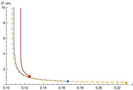
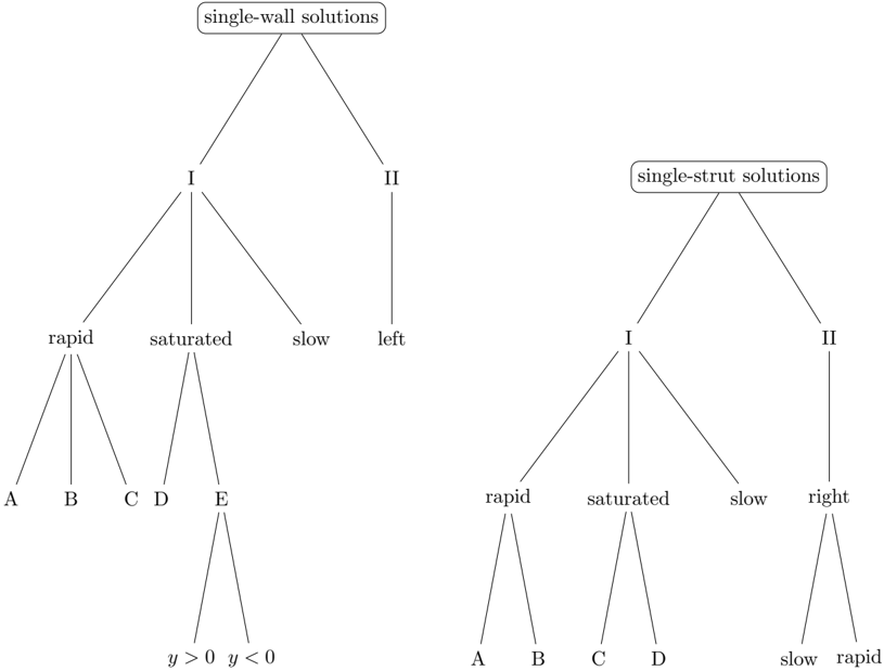
Figure 1 Classification of distinct single-wall and single-strut solutions with t timelike. Each leaf node represents a qualitatively-distinct solution.
Figure 1 Classification of distinct single-wall and single-strut solutions with t timelike. Each leaf node represents a qualitatively-distinct solution.CC-BY · From the PDF
Image 2
CC-BY · From the PDF
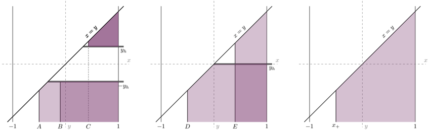
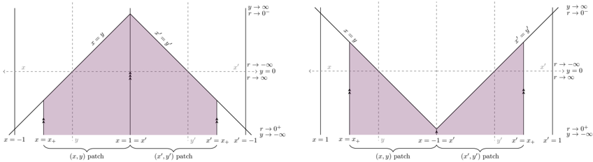
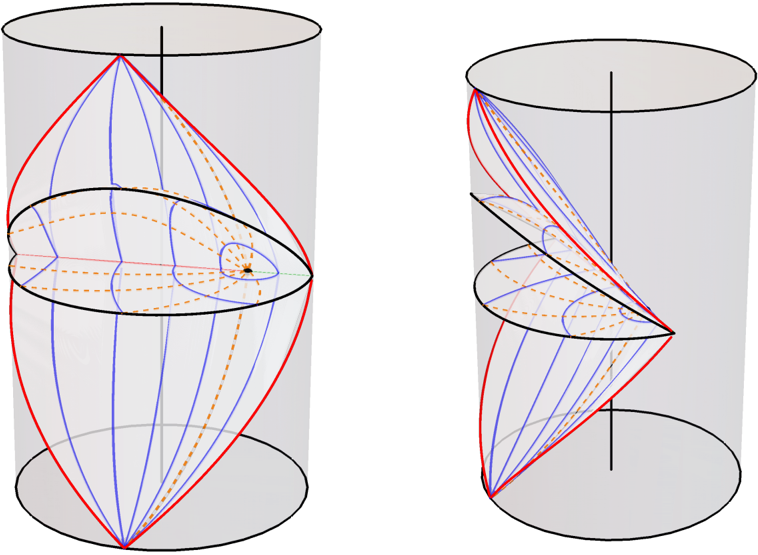
Figure 2 Coordinate ranges for single-wall solutions constructed from metrics of Class I (with t timelike). Left: three qualitatively distinct solutions are shown for class I rapid , Centre: three for class I saturated , and Right: one for class I slow .
Figure 2 Coordinate ranges for single-wall solutions constructed from metrics of Class I (with t timelike). Left: three qualitatively distinct solutions are shown for class I rapid , Centre: three for class I saturated , and Right: one for class I slow .CC-BY · From the PDF
Image 4
CC-BY · From the PDF
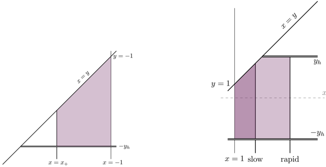
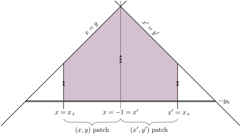
Figure 5 The two patches of type I spacetime used to construct a slowly accelerating conical defect. Left: Point particle pulled by a domain wall. Right: Point particle pushed by a strut-wall.
Figure 5 The two patches of type I spacetime used to construct a slowly accelerating conical defect. Left: Point particle pulled by a domain wall. Right: Point particle pushed by a strut-wall.CC-BY · From the PDF
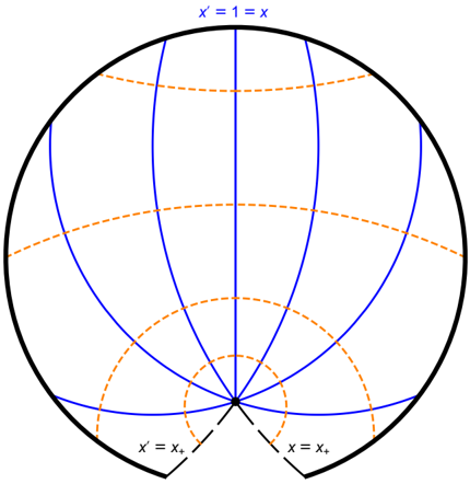
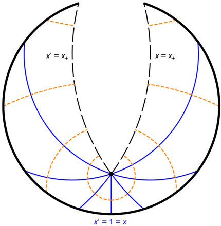
Figure 6 The slowly accelerating conical deficit with A = 0 . 9 ℓ , pulled by a wall, mapped onto the Poincar´ e disk. The deficit is shown as a black point and accelerates southwards. A 'wedge' is removed from the global space, with its edges x = x + and x ′ = x + (long-dashed black) identified to attain a wall. Several lines of constant x are shown in blue, with lines of constant y in dashed orange.
Figure 6 The slowly accelerating conical deficit with A = 0 . 9 ℓ , pulled by a wall, mapped onto the Poincar´ e disk. The deficit is shown as a black point and accelerates southwards. A 'wedge' is removed from the global space, with its edges x = x + and x ′ = x + (long-dashed black) identified to attain a wall. Several lines of constant x are shown in blue, with lines of constant y in dashed orange.CC-BY · From the PDF
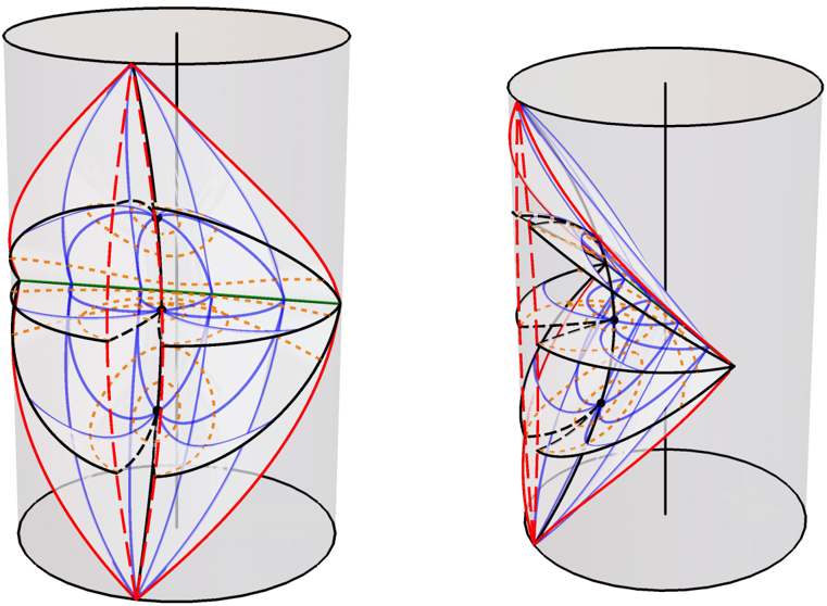
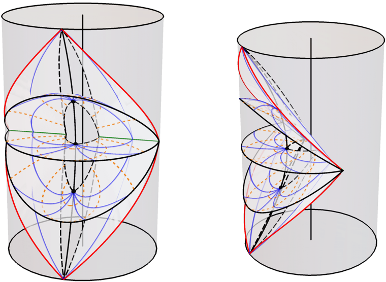
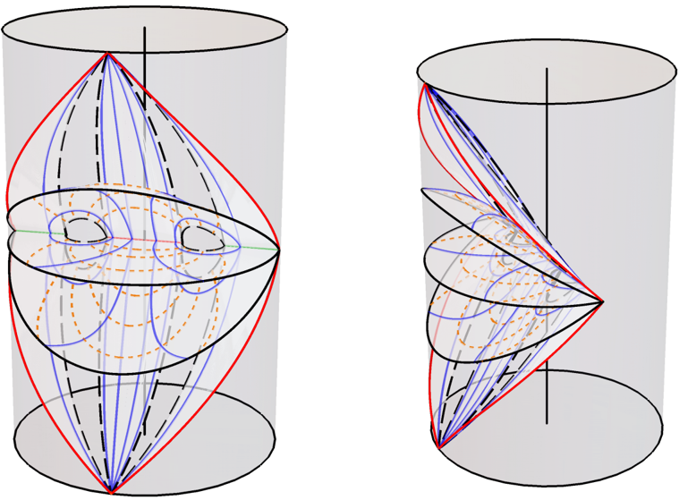
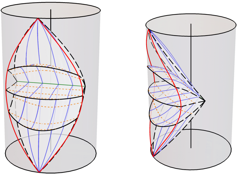
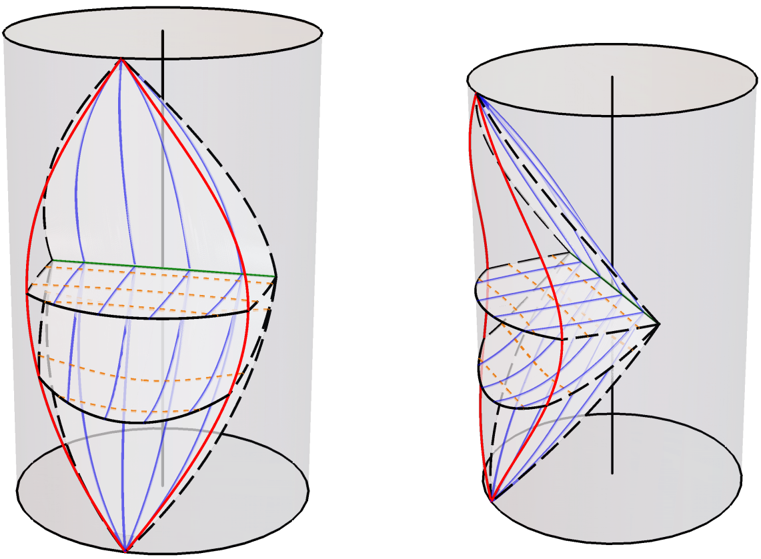
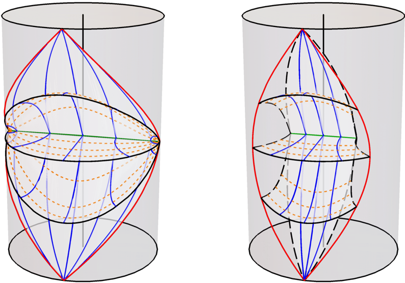
Figure 7 The Class I rapid,A solution embedded within global AdS 3 . The particle worldline is shown in solid black. Several surfaces of constant t are plotted. The event horizons are demonstrated by the surfaces at early and late t . The bifurcation surface is shown as a green line. A 'wedge' is removed, with its edges x = x + and x ′ = x + identified; this is the location of the domain wall. These edges are shown in long-dashed black within each time-slice, and in dashed red at the boundary. The boundary of the classically accessible subset of the global boundary is shown in red. Lines of constant x are shown in blue, with lines of constant y in dashed orange. To guide the eye, the axis of the cylinder is also shown in black.
Figure 7 The Class I rapid,A solution embedded within global AdS 3 . The particle worldline is shown in solid black. Several surfaces of constant t are plotted. The event horizons are demonstrated by the surfaces at early and late t . The bifurcation surface is shown as a green line. A 'wedge' is removed, with its edges x = x + and x ′ = x + identified; this is the location of the domain wall. These edges are shown in long-dashed black within each time-slice, and in dashed red at the boundary. The boundary of the classically accessible subset of the global boundary is shown in red. Lines of constant x are shown in blue, with lines of constant y in dashed orange. To guide the eye, the axis of the cylinder is also shown in black.CC-BY · From the PDF
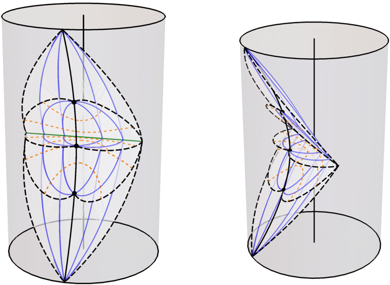
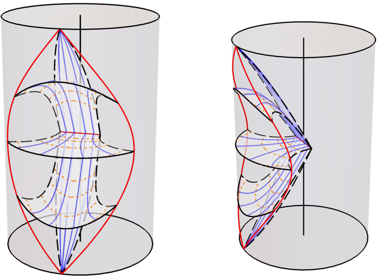
Figure 8 The Class I rapid,B solution embedded within global AdS 3 . The particle worldline is shown in solid black. Several surfaces of constant t are plotted. The event horizons are demonstrated by the surfaces at early and late t . The bifurcation surface is shown as a green line. The surfaces x = x + and x ′ = x + identified. Lines of constant t within these surfaces are shown in long-dashed black. None of the conformal boundary is included in the solution. Lines of constant x are shown in blue, with lines of constant y in dashed orange. To guide the eye, the axis of the cylinder is also shown in black.
Figure 8 The Class I rapid,B solution embedded within global AdS 3 . The particle worldline is shown in solid black. Several surfaces of constant t are plotted. The event horizons are demonstrated by the surfaces at early and late t . The bifurcation surface is shown as a green line. The surfaces x = x + and x ′ = x + identified. Lines of constant t within these surfaces are shown in long-dashed black. None of the conformal boundary is included in the solution. Lines of constant x are shown in blue, with lines of constant y in dashed orange. To guide the eye, the axis of the cylinder is also shown in black.CC-BY · From the PDF
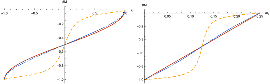
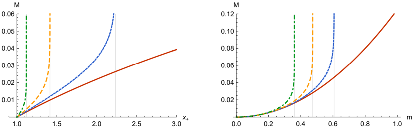
Figure 9 The holographic mass of the conical deficit pulled by a wall plotted as a function of x + (Left) and the local 'conical mass' m c (Right) with various acceleration parameters: A = 0 (solid red), A = 0 . 5 ℓ (dotted blue), A = 0 . 99 ℓ (dashed orange).
Figure 9 The holographic mass of the conical deficit pulled by a wall plotted as a function of x + (Left) and the local 'conical mass' m c (Right) with various acceleration parameters: A = 0 (solid red), A = 0 . 5 ℓ (dotted blue), A = 0 . 99 ℓ (dashed orange).CC-BY · From the PDF
Figure 10 The slowly accelerating conical deficit with A = 0 . 9 ℓ , pushed by a strut, mapped onto the Poincar´ e disk. The deficit is shown as a black point and accellerates southwards. A 'wedge' is removed from the global space, with its edges x = x + and x ′ = x + (long-dashed black) identified to attain a wall. Several lines of constant x are shown in blue, with lines of constant y in dashed orange.
Figure 10 The slowly accelerating conical deficit with A = 0 . 9 ℓ , pushed by a strut, mapped onto the Poincar´ e disk. The deficit is shown as a black point and accellerates southwards. A 'wedge' is removed from the global space, with its edges x = x + and x ′ = x + (long-dashed black) identified to attain a wall. Several lines of constant x are shown in blue, with lines of constant y in dashed orange.CC-BY · From the PDF
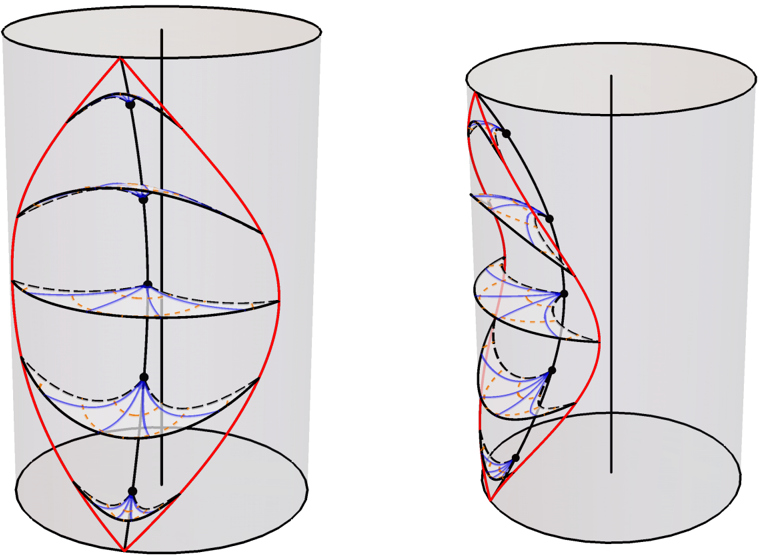
Figure 11 The rapidly accelerating light conical deficit with A > ℓ -1 , pushed by a strut, embedded within global AdS 3 . The deficit's worldline is shown in solid black. Several surfaces of constant t are plotted. The event horizon is demonstrated by the surfaces at early and late t . The bifurcation surface is shown as a green line. A 'wedge' is removed, with its faces x = x + and x ′ = x + identified. These faces are indicated by long-dashed black curves within each time-slice, and in dashed red at the boundary. The boundary of the classically accessible subset of the global boundary is shown in solid red. Lines of constant x are shown in blue, with lines of constant y in dashed orange. To guide the eye, the axis of the cylinder is also shown in black.
Figure 11 The rapidly accelerating light conical deficit with A > ℓ -1 , pushed by a strut, embedded within global AdS 3 . The deficit's worldline is shown in solid black. Several surfaces of constant t are plotted. The event horizon is demonstrated by the surfaces at early and late t . The bifurcation surface is shown as a green line. A 'wedge' is removed, with its faces x = x + and x ′ = x + identified. These faces are indicated by long-dashed black curves within each time-slice, and in dashed red at the boundary. The boundary of the classically accessible subset of the global boundary is shown in solid red. Lines of constant x are shown in blue, with lines of constant y in dashed orange. To guide the eye, the axis of the cylinder is also shown in black.CC-BY · From the PDF
Figure 12 The rapidly accelerating heavy conical deficit with A > ℓ -1 , pushed by a strut, embedded within global AdS 3 . The deficit's worldline is shown in solid black. Several surfaces of constant t are plotted. The surfaces x = x + and x ′ = x + are identified. Edges of x = x + are shown in long-dashed black within each time-slice. x + is taken positive enough that the entirety of the boundary is removed from the space before identification. The boundary of the classically accessible subset of the global boundary is shown in red. Lines of constant x are shown in blue, with lines of constant y in dashed orange. To guide the eye, the axis of the cylinder is also shown in black.
Figure 12 The rapidly accelerating heavy conical deficit with A > ℓ -1 , pushed by a strut, embedded within global AdS 3 . The deficit's worldline is shown in solid black. Several surfaces of constant t are plotted. The surfaces x = x + and x ′ = x + are identified. Edges of x = x + are shown in long-dashed black within each time-slice. x + is taken positive enough that the entirety of the boundary is removed from the space before identification. The boundary of the classically accessible subset of the global boundary is shown in red. Lines of constant x are shown in blue, with lines of constant y in dashed orange. To guide the eye, the axis of the cylinder is also shown in black.CC-BY · From the PDF
Image 13
CC-BY · From the PDF
Figure 14 The Class II right, slow black hole. Several surfaces of constant t are shown. The lines x = x + < y h are shown in dashed black, and are identified with their partner within the same time slice, wrapping the bifurcation surface (shown as a horizontal red line) into a circle. The early and late time-slices demonstrate the event horizon. Lines of constant y are shown in dashed orange. Lines of constant x are shown in blue. The classically accessible region of the boundary is delimited in red.
Figure 14 The Class II right, slow black hole. Several surfaces of constant t are shown. The lines x = x + < y h are shown in dashed black, and are identified with their partner within the same time slice, wrapping the bifurcation surface (shown as a horizontal red line) into a circle. The early and late time-slices demonstrate the event horizon. Lines of constant y are shown in dashed orange. Lines of constant x are shown in blue. The classically accessible region of the boundary is delimited in red.CC-BY · From the PDF
Figure 15 The Class II right,rapid black hole. Several surfaces of constant t are shown. The lines x = x + < y h are shown in dashed black, and are identified with their partner within the same time slice. The early and late time-slices show the event horizons. The black hole event horizon has a compact bifurcation surface with topology S 1 , shown in red, while the green line denotes the 'acceleration horizon' or droplet's bifurcation line with topology R . Lines of constant y are shown in dashed orange. Lines of constant x are shown in blue. The classically accessible region of the boundary is delimited in red.
Figure 15 The Class II right,rapid black hole. Several surfaces of constant t are shown. The lines x = x + < y h are shown in dashed black, and are identified with their partner within the same time slice. The early and late time-slices show the event horizons. The black hole event horizon has a compact bifurcation surface with topology S 1 , shown in red, while the green line denotes the 'acceleration horizon' or droplet's bifurcation line with topology R . Lines of constant y are shown in dashed orange. Lines of constant x are shown in blue. The classically accessible region of the boundary is delimited in red.CC-BY · From the PDF
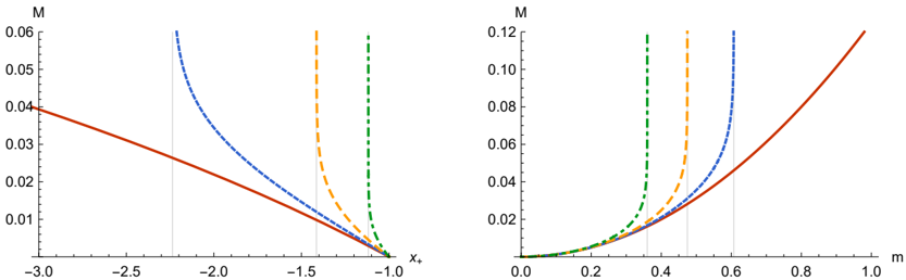
Figure 16 The holographic mass M of the BTZ black-hole pushed by a strut at various values of the acceleration parameter: A = 0 (solid red), A = 0 . 5 ℓ -1 (dotted blue), A = ℓ -1 (dashed orange), A = 2 ℓ -1 (dot-dashed green).
Figure 16 The holographic mass M of the BTZ black-hole pushed by a strut at various values of the acceleration parameter: A = 0 (solid red), A = 0 . 5 ℓ -1 (dotted blue), A = ℓ -1 (dashed orange), A = 2 ℓ -1 (dot-dashed green).CC-BY · From the PDF
Figure 17 The two patches of type II spacetime used to construct a black hole with a pulling wall.
Figure 17 The two patches of type II spacetime used to construct a black hole with a pulling wall.CC-BY · From the PDF
Figure 18 The Class II left black hole. Several surfaces of constant t are shown; those of large positive and negative t outline the event horizon. The surface x = x + - shown in dashed black - is identified with its partner within each time-slice. The bifurcation surface of the Killing horizon is shown in green and has topology S 1 . Lines of constant x and y are shown in solid blue and dashed orange respectively. The classically accessible region of the conformal boundary is delimited in red.
Figure 18 The Class II left black hole. Several surfaces of constant t are shown; those of large positive and negative t outline the event horizon. The surface x = x + - shown in dashed black - is identified with its partner within each time-slice. The bifurcation surface of the Killing horizon is shown in green and has topology S 1 . Lines of constant x and y are shown in solid blue and dashed orange respectively. The classically accessible region of the conformal boundary is delimited in red.CC-BY · From the PDF
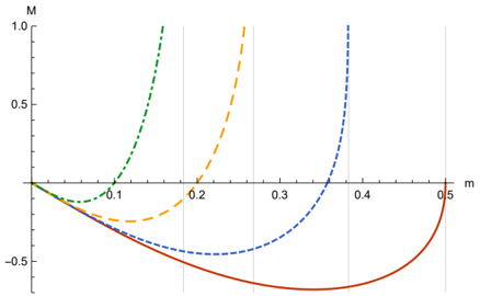
Figure 19 The holographic mass M of the BTZ black-hole pulled by a wall at various acceleration parameters: A = 0 (solid red), A = 0 . 5 ℓ -1 (dotted blue), A = ℓ -1 (dashed orange), A = 2 ℓ -1 (dot-dashed green).
Figure 19 The holographic mass M of the BTZ black-hole pulled by a wall at various acceleration parameters: A = 0 (solid red), A = 0 . 5 ℓ -1 (dotted blue), A = ℓ -1 (dashed orange), A = 2 ℓ -1 (dot-dashed green).CC-BY · From the PDF
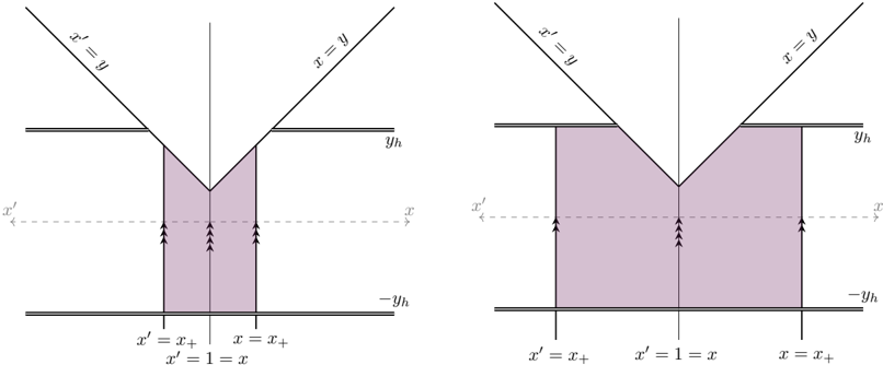
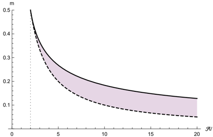
Figure 20 The parameter space of the I rapid,C solution (shaded purple).
Figure 20 The parameter space of the I rapid,C solution (shaded purple).CC-BY · From the PDF
Figure 21 The 'circumference' of loops of constant r . ℓ is set to unity with A = 10. Three values of m (6 -1 , 8 -1 , and 9 -1 ) are shown (in solid red, dotted blue, and dashed orange respectively). The value at the horizon radius r = r h is marked by a shape.
Figure 21 The 'circumference' of loops of constant r . ℓ is set to unity with A = 10. Three values of m (6 -1 , 8 -1 , and 9 -1 ) are shown (in solid red, dotted blue, and dashed orange respectively). The value at the horizon radius r = r h is marked by a shape.CC-BY · From the PDF
Figure 22 The Class I rapid,C solution, as a portion of global AdS 3 . Several surfaces of constant t are shown. The horizon is shown by the surfaces at early and late times, with the bifuration surface shown in green. The lines x = x + and x ′ = x + within each time-slice (shown in long-dashed black) are identified, which imbues the birfurcation surface with the topology of a circle. Lines of constant x are shown in blue, with lines of constant y shown in dashed orange. The classically accessible subset of the global boundary is delimited in red. To guide the eye, the locus of the cylinder is shown in solid black.
Figure 22 The Class I rapid,C solution, as a portion of global AdS 3 . Several surfaces of constant t are shown. The horizon is shown by the surfaces at early and late times, with the bifuration surface shown in green. The lines x = x + and x ′ = x + within each time-slice (shown in long-dashed black) are identified, which imbues the birfurcation surface with the topology of a circle. Lines of constant x are shown in blue, with lines of constant y shown in dashed orange. The classically accessible subset of the global boundary is delimited in red. To guide the eye, the locus of the cylinder is shown in solid black.CC-BY · From the PDF
Figure 23 A plot of 8 παM at various values of A ℓ : A ℓ = 2 . 0 (solid red), A ℓ = 2 . 8 (dotted blue), A ℓ = 5 . 0 (dashed orange), A ℓ = 10 (dot-dashed green). The grey vertical lines denote the asymptotes where the divergences A ℓ = ( m sin( mπ )) -1 are met. Negative values of M are forbidden by the lower bound m ≥ ( A ℓ ) -1 .
Figure 23 A plot of 8 παM at various values of A ℓ : A ℓ = 2 . 0 (solid red), A ℓ = 2 . 8 (dotted blue), A ℓ = 5 . 0 (dashed orange), A ℓ = 10 (dot-dashed green). The grey vertical lines denote the asymptotes where the divergences A ℓ = ( m sin( mπ )) -1 are met. Negative values of M are forbidden by the lower bound m ≥ ( A ℓ ) -1 .CC-BY · From the PDF
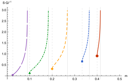
Figure 24 The entropy ℓ -1 S of the I rapid,C solution at various values of A ℓ : A ℓ = 2 . 5 (solid red), A ℓ = 3 . 0 (dotted blue), A ℓ = 5 . 0 (dashed orange), A ℓ = 10 (dot-dashed green), A ℓ = 40 (long-dashed purple). A solid grey vertical line denotes an asymptote where the divergence A ℓ = ( m sin( mπ )) -1 is met. A dashed grey line dentotes the value of m for a massless solution; the entropy at this point is marked with a shape.
Figure 24 The entropy ℓ -1 S of the I rapid,C solution at various values of A ℓ : A ℓ = 2 . 5 (solid red), A ℓ = 3 . 0 (dotted blue), A ℓ = 5 . 0 (dashed orange), A ℓ = 10 (dot-dashed green), A ℓ = 40 (long-dashed purple). A solid grey vertical line denotes an asymptote where the divergence A ℓ = ( m sin( mπ )) -1 is met. A dashed grey line dentotes the value of m for a massless solution; the entropy at this point is marked with a shape.CC-BY · From the PDF
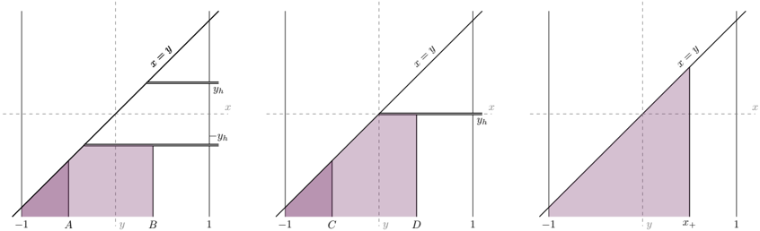
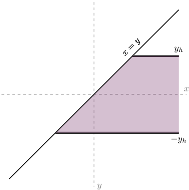
Figure 25 Coordinate ranges for the Class III solution.
Figure 25 Coordinate ranges for the Class III solution.CC-BY · From the PDF
Figure 26 The Class III solution. Several surfaces of constant τ are shown, with those at very early and very late times outlining the two disjoint bifurcate Killing horizons. The red bifurcation surface is y = -y h , while the green bifurcation surface is y = + y h . The black dot denotes the point x →∞ . Lines of constant finite x are shown in solid blue, with lines of constant y shown in dashed orange.
Figure 26 The Class III solution. Several surfaces of constant τ are shown, with those at very early and very late times outlining the two disjoint bifurcate Killing horizons. The red bifurcation surface is y = -y h , while the green bifurcation surface is y = + y h . The black dot denotes the point x →∞ . Lines of constant finite x are shown in solid blue, with lines of constant y shown in dashed orange.CC-BY · From the PDF
Figure 27 The planar and compact (static) BTZ black holes. Lines of constant φ are shown in blue, with lines of constant r in dashed orange. Several surfaces of constant time t are shown. The classically accesible subset of the boundary is bounded in red. To guide the eye, the locus of the cylinder is shown in solid black. (a): φ ∈ R , giving the planar BTZ geometry or 'Rindler wedge'. The bifurcation surface (green) has topology R . (b): φ identified with period 2 π , giving the BTZ black hole. Lines of constant t and φ = ± π are plotted in long-dashed black, pairs of which are identified across the same time-slice. The bifurcation surface (green) has topology S 1 .
Figure 27 The planar and compact (static) BTZ black holes. Lines of constant φ are shown in blue, with lines of constant r in dashed orange. Several surfaces of constant time t are shown. The classically accesible subset of the boundary is bounded in red. To guide the eye, the locus of the cylinder is shown in solid black. (a): φ ∈ R , giving the planar BTZ geometry or 'Rindler wedge'. The bifurcation surface (green) has topology R . (b): φ identified with period 2 π , giving the BTZ black hole. Lines of constant t and φ = ± π are plotted in long-dashed black, pairs of which are identified across the same time-slice. The bifurcation surface (green) has topology S 1 .CC-BY · From the PDF

Verification

Claims the paper makes

The claims and statistics of this paper haven’t been checked yet.

Run the check — free, no account needed. It reads the open-access text and checks the sources it cites.

A few free checks a day · papers already verified open instantly · results are public

Claims other papers make about this one

Each is checked against this paper’s own text: does it say what the citing paper says it does?

Self-check

Percentages, sums and reported differences re-computed from the paper’s own numbers.

The self-check needs the paper’s full text.

Citations

Cites

Show all 2 references

Research works printed but not linked: 53

  1. W. Kinnersley and M. Walker, Uniformly accelerating charged mass in general relativity, Phys. Rev. D 2 (1970) 1359 [INSPIRE]. · DOI
  2. J. Podolsky, Accelerating black holes in anti-de Sitter universe, Czech. J. Phys. 52 (2002) 1 [gr-qc/0202033] [INSPIRE]. · arXiv
  3. O.J.C. Dias and J.P.S. Lemos, Pair of accelerated black holes in anti-de Sitter background: AdS C metric, Phys. Rev. D 67 (2003) 064001 [hep-th/0210065] [INSPIRE]. · DOI
  4. J.F. Plebanski and M. Demianski, Rotating, charged, and uniformly accelerating mass in general relativity, Annals Phys. 98 (1976) 98 [INSPIRE]. · DOI · Paper page
  5. J.B. Griffiths and J. Podolsky, A New look at the Plebanski-Demianski family of solutions, Int. J. Mod. Phys. D 15 (2006) 335 [gr-qc/0511091] [INSPIRE]. · DOI
  6. M. Appels, R. Gregory and D. Kubiznak, Thermodynamics of Accelerating Black Holes, Phys. Rev. Lett. 117 (2016) 131303 [arXiv:1604.08812] [INSPIRE]. · DOI · Paper page
  7. M. Appels, R. Gregory and D. Kubiznak, Black Hole Thermodynamics with Conical Defects, JHEP 05 (2017) 116 [arXiv:1702.00490] [INSPIRE]. · DOI · Paper page
  8. A. Anabalón, M. Appels, R. Gregory, D. Kubizňák, R.B. Mann and A. Ovgün, Holographic Thermodynamics of Accelerating Black Holes, Phys. Rev. D 98 (2018) 104038 [arXiv:1805.02687] [INSPIRE]. · DOI · Paper page
  9. A. Anabalón, F. Gray, R. Gregory, D. Kubizňák and R.B. Mann, Thermodynamics of Charged, Rotating, and Accelerating Black Holes, JHEP 04 (2019) 096 [arXiv:1811.04936] [INSPIRE]. · DOI
  10. R. Gregory, Z.L. Lim and A. Scoins, Thermodynamics of Many Black Holes, Front. in Phys. 9 (2021) 187 [arXiv:2012.15561] [INSPIRE]. · DOI
  11. A. Ball and N. Miller, Accelerating black hole thermodynamics with boost time, Class. Quant. Grav. 38 (2021) 145031 [arXiv:2008.03682] [INSPIRE]. · DOI · Paper page
  12. R. Gregory and A. Scoins, Accelerating Black Hole Chemistry, Phys. Lett. B 796 (2019) 191 [arXiv:1904.09660] [INSPIRE]. · DOI
  13. P. Krtouš and A. Zelnikov, Thermodynamics of two black holes, JHEP 02 (2020) 164 [arXiv:1909.13467] [INSPIRE]. · DOI
  14. J.M. Maldacena, The Large N limit of superconformal field theories and supergravity, Adv. Theor. Math. Phys. 2 (1998) 231 [hep-th/9711200] [INSPIRE]. · DOI · Paper page
  15. P. Ferrero, J.P. Gauntlett, J.M.P. Ipiña, D. Martelli and J. Sparks, Accelerating black holes and spinning spindles, Phys. Rev. D 104 (2021) 046007 [arXiv:2012.08530] [INSPIRE]. · DOI
  16. M.H. Dehghani, A.M. Ghezelbash and R.B. Mann, Vortex holography, Nucl. Phys. B 625 (2002) 389 [hep-th/0105134] [INSPIRE]. · DOI
  17. O.J.C. Dias, G.T. Horowitz, N. Iqbal and J.E. Santos, Vortices in holographic superfluids and superconductors as conformal defects, JHEP 04 (2014) 096 [arXiv:1311.3673] [INSPIRE]. · DOI
  18. S. Deser and R. Jackiw, Three-Dimensional Cosmological Gravity: Dynamics of Constant Curvature, Annals Phys. 153 (1984) 405 [INSPIRE]. · DOI · Paper page
  19. M. Bañados, C. Teitelboim and J. Zanelli, The Black hole in three-dimensional space-time, Phys. Rev. Lett. 69 (1992) 1849 [hep-th/9204099] [INSPIRE]. · DOI · Paper page
  20. M. Bañados, M. Henneaux, C. Teitelboim and J. Zanelli, Geometry of the (2 + 1) black hole, Phys. Rev. D 48 (1993) 1506 [Erratum ibid. 88 (2013) 069902] [gr-qc/9302012] [INSPIRE]. · DOI · Paper page
  21. A. Maloney and E. Witten, Quantum Gravity Partition Functions in Three Dimensions, JHEP 02 (2010) 029 [arXiv:0712.0155] [INSPIRE]. · DOI
  22. V.E. Hubeny, D. Marolf and M. Rangamani, Black funnels and droplets from the AdS C-metrics, Class. Quant. Grav. 27 (2010) 025001 [arXiv:0909.0005] [INSPIRE]. · DOI · Paper page
  23. V.E. Hubeny, D. Marolf and M. Rangamani, Hawking radiation in large N strongly-coupled field theories, Class. Quant. Grav. 27 (2010) 095015 [arXiv:0908.2270] [INSPIRE]. · DOI · Paper page
  24. M. Astorino, Accelerating black hole in 2 + 1 dimensions and 3 + 1 black (st)ring, JHEP 01 (2011) 114 [arXiv:1101.2616] [INSPIRE]. · DOI · Paper page
  25. M.M. Anber, AdS4/CFT3 + Gravity for Accelerating Conical Singularities, JHEP 11 (2008) 026 [arXiv:0809.2789] [INSPIRE]. · DOI
  26. W. Xu, K. Meng and L. Zhao, Accelerating BTZ spacetime, Class. Quant. Grav. 29 (2012) 155005 [arXiv:1111.0730] [INSPIRE]. · DOI · Paper page
  27. W. Israel, Singular hypersurfaces and thin shells in general relativity, Nuovo Cim. B 44S10 (1966) 1 [Erratum ibid. 48 (1967) 463] [INSPIRE]. · DOI · Paper page
  28. L. Randall and R. Sundrum, An Alternative to compactification, Phys. Rev. Lett. 83 (1999) 4690 [hep-th/9906064] [INSPIRE]. · DOI · Paper page
  29. L. Randall and R. Sundrum, A Large mass hierarchy from a small extra dimension, Phys. Rev. Lett. 83 (1999) 3370 [hep-ph/9905221] [INSPIRE]. · DOI · Paper page
  30. S. Deser, R. Jackiw and G. ’t Hooft, Three-Dimensional Einstein Gravity: Dynamics of Flat Space, Annals Phys. 152 (1984) 220 [INSPIRE]. · DOI · Paper page
  31. M.M. Caldarelli, G. Cognola and D. Klemm, Thermodynamics of Kerr-Newman-AdS black holes and conformal field theories, Class. Quant. Grav. 17 (2000) 399 [hep-th/9908022] [INSPIRE]. · DOI · Paper page
  32. J.B. Griffiths, P. Krtous and J. Podolsky, Interpreting the C-metric, Class. Quant. Grav. 23 (2006) 6745 [gr-qc/0609056] [INSPIRE]. · DOI
  33. V. Balasubramanian and P. Kraus, A Stress tensor for Anti-de Sitter gravity, Commun. Math. Phys. 208 (1999) 413 [hep-th/9902121] [INSPIRE]. · DOI · Paper page
  34. J.D. Brown and J.W. York, Jr., Quasilocal energy and conserved charges derived from the gravitational action, Phys. Rev. D 47 (1993) 1407 [gr-qc/9209012] [INSPIRE]. · DOI · Paper page
  35. R.B. Mann, Misner string entropy, Phys. Rev. D 60 (1999) 104047 [hep-th/9903229] [INSPIRE]. · DOI
  36. M. Henningson and K. Skenderis, The Holographic Weyl anomaly, JHEP 07 (1998) 023 [hep-th/9806087] [INSPIRE]. · DOI · Paper page
  37. S. de Haro, S.N. Solodukhin and K. Skenderis, Holographic reconstruction of space-time and renormalization in the AdS/CFT correspondence, Commun. Math. Phys. 217 (2001) 595 [hep-th/0002230] [INSPIRE]. · DOI · Paper page
  38. R. Blumenhagen and E. Plauschinn, Introduction to Conformal Field Theory: With Applications to String Theory, Lect. Notes Phys. 779 (2009) 1. · DOI
  39. M. Bañados, Three-dimensional quantum geometry and black holes, AIP Conf. Proc. 484 (1999) 147 [hep-th/9901148] [INSPIRE]. · DOI
  40. M. Bañados, Notes on black holes and three-dimensional gravity, AIP Conf. Proc. 490 (1999) 198 [hep-th/9903244] [INSPIRE]. · DOI
  41. I. Papadimitriou and K. Skenderis, Thermodynamics of asymptotically locally AdS spacetimes, JHEP 08 (2005) 004 [hep-th/0505190] [INSPIRE]. · DOI
  42. S. Carlip, Lectures on (2 + 1) dimensional gravity, J. Korean Phys. Soc. 28 (1995) S447 [gr-qc/9503024] [INSPIRE]. · arXiv
  43. A.M. Frassino, R.B. Mann and J.R. Mureika, Lower-Dimensional Black Hole Chemistry, Phys. Rev. D 92 (2015) 124069 [arXiv:1509.05481] [INSPIRE]. · DOI
  44. P. Krtous, Accelerated black holes in an anti-de Sitter universe, Phys. Rev. D 72 (2005) 124019 [gr-qc/0510101] [INSPIRE]. · DOI
  45. D. Cassani, J.P. Gauntlett, D. Martelli and J. Sparks, Thermodynamics of accelerating and supersymmetric AdS4 black holes, Phys. Rev. D 104 (2021) 086005 [arXiv:2106.05571] [INSPIRE]. · DOI
  46. K. Hong and E. Teo, A New form of the C metric, Class. Quant. Grav. 20 (2003) 3269 [gr-qc/0305089] [INSPIRE]. · DOI · Paper page
  47. M. Astorino, Thermodynamics of Regular Accelerating Black Holes, Phys. Rev. D 95 (2017) 064007 [arXiv:1612.04387] [INSPIRE]. · DOI
  48. M. Astorino, CFT Duals for Accelerating Black Holes, Phys. Lett. B 760 (2016) 393 [arXiv:1605.06131] [INSPIRE]. · DOI
  49. C. Martinez and J. Zanelli, Back reaction of a conformal field on a three-dimensional black hole, Phys. Rev. D 55 (1997) 3642 [gr-qc/9610050] [INSPIRE]. · DOI
  50. M. Casals, A. Fabbri, C. Martínez and J. Zanelli, Quantum Backreaction on Three-Dimensional Black Holes and Naked Singularities, Phys. Rev. Lett. 118 (2017) 131102 [arXiv:1608.05366] [INSPIRE]. · DOI
  51. R. Emparan, G.T. Horowitz and R.C. Myers, Exact description of black holes on branes, JHEP 01 (2000) 007 [hep-th/9911043] [INSPIRE]. · DOI · Paper page
  52. R. Emparan, A.M. Frassino and B. Way, Quantum BTZ black hole, JHEP 11 (2020) 137 [arXiv:2007.15999] [INSPIRE]. · DOI · Paper page
  53. H. Kudoh and Y. Kurita, Thermodynamics of four-dimensional black objects in the warped compactification, Phys. Rev. D 70 (2004) 084029 [gr-qc/0406107] [INSPIRE]. · DOI · Paper page

Cited by

Sorted by citations

See all 26

Metadata

Authors
Arenas-Henriquez, G., Gregory, R., & Scoins, A.
Venue
Journal of High Energy Physics
Published
2022-05-10
Volume
2022
Issue
5
ISSN
1029-8479
Cited by
26
References
2
Language
en

About these checks

Registry, retraction, Cites and statistics results are computed, not judged, with one exception: a printed reference that no index lists is read once by a model before it counts as a citation error. Claims are extracted by a model and kept only when their quote appears verbatim in the text; each cited source is then checked, with a model’s help, for whether it says what the claim relies on. Those verdicts can be wrong — read the claim’s quote and the cited source before relying on one.

Statistics and arithmetic are recomputed, not judged.

Confidence bands are shown only for fields calibrated on our annotated test set. None is calibrated yet, so no band is shown.

What counts as a claim ›How we measure confidence ›How we check this ›

Are you an author, or do you see a problem with this page? Request a review

How to cite

Cite CoChat for the checks on this page, and the paper for its own findings.

This page
CoChat. (2026). Citation check: On acceleration in three dimensions. https://app.cochat.ai/papers/10.1007/jhep05(2022)063
The paper
Arenas-Henriquez, G., Gregory, R., & Scoins, A. (2022). On acceleration in three dimensions. Journal of High Energy Physics. https://doi.org/10.1007/jhep05(2022)063