Student or educator? Sign up with your school email and get 6 months of Pro free.
CoChat

The DOI matches its Crossref record; 61 of the 61 references it cites were found in a registry or an index; 28 of the 43 sources its claims cite were checked for support.

A population code for spatial representation in the zebrafish telencephalon

Open access
Yang, Chuyu, Mammen, Lorenz, Kim, Byoungsoo, Li, Meng, Robson, Drew N., Li, Jennifer M. · 2024 · Nature

Abstract

Abstract Spatial learning in teleost fish requires an intact telencephalon 1 , a brain region that contains putative analogues to components of the mammalian limbic system (for example, hippocampus) 2–4 . However, cells fundamental to spatial cognition in mammals—for example, place cells (PCs) 5,6 —have yet to be established in any fish species. In this study, using tracking microscopy to record brain-wide calcium activity in freely swimming larval zebrafish 7 , we compute the spatial information content 8 of each neuron across the brain. Strikingly, in every recorded animal, cells with the highest spatial specificity were enriched in the zebrafish telencephalon. These PCs form a population code of space from which we can decode the animal’s spatial location across time. By continuous recording of population-level activity, we found that the activity manifold of PCs refines and untangles over time. Through systematic manipulation of allothetic and idiothetic cues, we demonstrate that zebrafish PCs integrate multiple sources of information and can flexibly remap to form distinct spatial maps. Using analysis of neighbourhood distance between PCs across environments, we found evidence for a weakly preconfigured network in the telencephalon. The discovery of zebrafish PCs represents a step forward in our understanding of spatial cognition across species and the functional role of the early vertebrate telencephalon.

Overview

CoChat Summary

## TL;DR

Using brain-wide calcium imaging in freely swimming larval zebrafish, the authors identify spatially tuned neurons in the telencephalon that behave like place cells and together form a population code for location. They show this code can decode position, refines over time, integrates self-motion and visual cues, and remaps across environments.

## Key findings

  • In every recorded animal, the telencephalon contained the highest number and fraction of place cells, with 69 ± 14% of PCs there even though telencephalic neurons were only 8 ± 1% of recorded neurons on average.
  • A linear decoder using telencephalic PCs predicted position with 6.82 ± 2.05 mm median ± s.d. error; using the top 1,000 cells across the whole brain gave 6.69 ± 2.34 mm, while a minimal set of 25 PCs achieved 5.41 ± 0.81 mm mean ± s.d. error.
  • Across a 90 min session, the spatial activity manifold became more “untangled,” with neighbourhood distance decreasing significantly in 6 of 7 animals (P < 10−3), alongside increased spatial specificity (P < 0.01 for 7/7) and decreased decoding error (P < 10−5 for 5/7).
  • Place-field stability survived changes in illumination, landmark removal, and boundary morphing, with reported PF correlations of 0.66, 0.54, and 0.44 (or 0.40, 0.35, 0.44 in the interruption-of-path-integration recovery experiments, depending on manipulation), indicating both idiothetic and allocentric inputs contribute.
  • When chamber geometry and landmarks were made completely distinct and path integration was interrupted, spatial maps remapped strongly: PF correlation 0.13 and PV correlation 0.05, compared with within-session controls of 0.56 and 0.58.
  • Neighbourhood relationships between PCs were partially maintained across remapping: retention was significantly below within-session controls (P < 10−5, four of four fish) but still above random chance (P < 10−5, four of four fish), suggesting weak preconfiguration.

## Methods

  • Freely swimming larval zebrafish expressing pan-neuronal GCaMP indicators were imaged with tracking microscopy in custom chambers; recordings used brain-wide calcium imaging at 2 volumes/s, with individual sessions lasting 45–100 min and an exploration session of 90 min in the main paradigm.
  • Neurons were extracted with constrained non-negative matrix factorization, place cells were defined by spatial specificity criteria based on shuffled null distributions, and analyses used spatial activity maps, decoder-based position prediction, Isomap embeddings, and PF/PV correlation metrics.
  • Manipulations included light-to-dark transitions, landmark removal, wall insertion/removal, chamber morphing, whole-chamber rotation, wall-only rotation, and ABA/novel-environment remapping to separate idiothetic from allocentric contributions.

## Limitations

  • The paper states that further research is needed to determine how fully zebrafish PCs are analogous to mammalian PCs, including their storage capacity and stability across multiple environments, developmental stages, and days/weeks.
  • It also notes that the work primarily focused on exposure to an initially new environment, so broader generalization is not yet tested.
  • Evident from the text: the study is performed in larval zebrafish under tether-free imaging in custom chambers, so the findings may not directly generalize to adult fish or natural habitats (inferred from the experimental design, not explicitly framed as a limitation).

Model-written summary. Check it against the paper before relying on it.

Integrity signals

Registry

Crossref · 10.1038/s41586-024-07867-2

Cites

61 of 61 references verified0 citation errors · 0 not checkable

Statistics

Nothing to recompute.

Figures

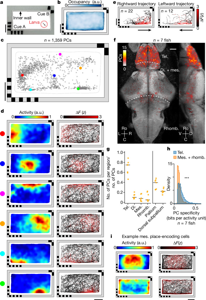
Fig. 1 Identification of PCs in the larval zebrafish brain. a, Rectangular behavioural arena with two landmark cues containing different visual patterns on opposing corners. There is a transparent inner polydimethylsiloxane (PDMS) wall (1.5 mm wide) preventing the animal from directly contacting the landmarks. b, Normalized median chamber occupancy across seven animals. c, Distribution of PF COM for all PCs with a confined PF in an example fish (Methods). Each dot represents the COM of one cell’s PF (Methods). The six example cells (coloured dots) are shown in d. d, Spatial activity maps (left, averaged neural response by location; Methods) and corresponding animal trajectories (right, colour coded by neural activity) are shown for six example cells from c. e, Responses of an example cell with a non-directional PF for two orientations of traversal (leftwards and rightwards) through the PF. Traversals across the 90 min experiment are colour coded by neural activity. Orientation is classified by the animal’s heading as it enters the PF. f, Anatomical distribution of PCs across seven animals plotted on the reference brain (maximum projection; Methods). g, Fraction of all PCs identified anywhere in the brain that are found in each brain region. Each animal is shown individually (orange dots, n = 7 animals), along with the median across animals (black lines). Anatomical subdivisions of the telencephalon (pallium and dorsal subpallium; Extended Data Fig. 2b) are plotted separately. h, Comparison of spatial specificity for PCs found in the telencephalon and for those found in the mesencephalon and rhombencephalon (n = 7 animals, P = 8.4 × 10−124, one-sided Mann–Whitney U-test). i, Spatial activity maps and animal trajectories for two example mesencephalic cells with significant spatial information encoding the interior (top) and periphery of the chamber (bottom). Scale bars, 10 mm (a–e,i), 50 µm (f). a.u., arbitrary units. di., diencephalon; mes., mesencephalon; rhomb., rhombencephalon; tel., telencephalon. Source Data
Fig. 1 Identification of PCs in the larval zebrafish brain. a, Rectangular behavioural arena with two landmark cues containing different visual patterns on opposing corners. There is a transparent inner polydimethylsiloxane (PDMS) wall (1.5 mm wide) preventing the animal from directly contacting the landmarks. b, Normalized median chamber occupancy across seven animals. c, Distribution of PF COM for all PCs with a confined PF in an example fish (Methods). Each dot represents the COM of one cell’s PF (Methods). The six example cells (coloured dots) are shown in d. d, Spatial activity maps (left, averaged neural response by location; Methods) and corresponding animal trajectories (right, colour coded by neural activity) are shown for six example cells from c. e, Responses of an example cell with a non-directional PF for two orientations of traversal (leftwards and rightwards) through the PF. Traversals across the 90 min experiment are colour coded by neural activity. Orientation is classified by the animal’s heading as it enters the PF. f, Anatomical distribution of PCs across seven animals plotted on the reference brain (maximum projection; Methods). g, Fraction of all PCs identified anywhere in the brain that are found in each brain region. Each animal is shown individually (orange dots, n = 7 animals), along with the median across animals (black lines). Anatomical subdivisions of the telencephalon (pallium and dorsal subpallium; Extended Data Fig. 2b) are plotted separately. h, Comparison of spatial specificity for PCs found in the telencephalon and for those found in the mesencephalon and rhombencephalon (n = 7 animals, P = 8.4 × 10−124, one-sided Mann–Whitney U-test). i, Spatial activity maps and animal trajectories for two example mesencephalic cells with significant spatial information encoding the interior (top) and periphery of the chamber (bottom). Scale bars, 10 mm (a–e,i), 50 µm (f). a.u., arbitrary units. di., diencephalon; mes., mesencephalon; rhomb., rhombencephalon; tel., telencephalon. Source DataCC BY · PubMed Central
Fig. 2 Physical location of larval zebrafish can be decoded from the population activity of PCs. a, Distribution of binarized telencephalic PFs in the chamber (median across animals). b, Median decoder error across animals at each bin within the chamber. To decode the physical location of the animal, a direct basis decoder was applied to telencephalic PCs (Methods). For all panels except f,g, the 1,000 cells with the highest spatial specificity were used as input to the decoder. c, Example traces show the x (top) and y (bottom) coordinates of the true (black) and decoded (red) animal locations. d, Activity of PCs across the final 3 min of c, together with true x (top) and y (bottom) coordinates of the animal (white overlay). Activity is shown two ways, sorting each cell by either the x or y component of its PF’s COM. e, Decoding performance for cells from different brain regions: PCs across the entire brain (PC), telencephalic PCs (Tel. PC), mes- and rhombencephalic PCs (M + R PC) and optic tectum cells (OT cells). Three controls are shown: random non-PCs (control 1, C1), uniformly random chamber positions (control 2, C2) and centroid of the animal’s spatial occupancy map (control 3, C3). Black horizontal bars represent median across animals. f, Decoder error as a function of the number of telencephalic cells included, in descending order of spatial tuning (Methods). Solid line indicates the mean and the shaded region indicates s.d. (the same applies to g). g, Decoder error as a function of the number of PCs included, using greedy selection to minimize redundancy (Methods). h, Distribution of decoder error across time (pooled across animals). Vertical solid line denotes median error, dashed line the behaviour-informed baseline and dotted line the accessible length of the chamber long axis. Scale bars, 10 mm. Source Data
Fig. 2 Physical location of larval zebrafish can be decoded from the population activity of PCs. a, Distribution of binarized telencephalic PFs in the chamber (median across animals). b, Median decoder error across animals at each bin within the chamber. To decode the physical location of the animal, a direct basis decoder was applied to telencephalic PCs (Methods). For all panels except f,g, the 1,000 cells with the highest spatial specificity were used as input to the decoder. c, Example traces show the x (top) and y (bottom) coordinates of the true (black) and decoded (red) animal locations. d, Activity of PCs across the final 3 min of c, together with true x (top) and y (bottom) coordinates of the animal (white overlay). Activity is shown two ways, sorting each cell by either the x or y component of its PF’s COM. e, Decoding performance for cells from different brain regions: PCs across the entire brain (PC), telencephalic PCs (Tel. PC), mes- and rhombencephalic PCs (M + R PC) and optic tectum cells (OT cells). Three controls are shown: random non-PCs (control 1, C1), uniformly random chamber positions (control 2, C2) and centroid of the animal’s spatial occupancy map (control 3, C3). Black horizontal bars represent median across animals. f, Decoder error as a function of the number of telencephalic cells included, in descending order of spatial tuning (Methods). Solid line indicates the mean and the shaded region indicates s.d. (the same applies to g). g, Decoder error as a function of the number of PCs included, using greedy selection to minimize redundancy (Methods). h, Distribution of decoder error across time (pooled across animals). Vertical solid line denotes median error, dashed line the behaviour-informed baseline and dotted line the accessible length of the chamber long axis. Scale bars, 10 mm. Source DataCC BY · PubMed Central
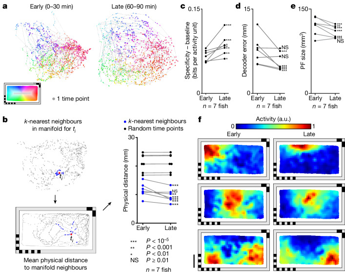
Fig. 3 Activity manifold of PCs untangles across time. a, Change in manifold structure across two stages of the experiment (early, 0–30 min; late, 60–90 min). Individual time points are colour coded by the animal’s location within the behavioural arena. b, Mean physical distance to 30 neighbouring points in the two-dimensional manifold space, averaged across all time points (left). Change in this distance between early and late stages of the experiment (blue) and baseline (black, 30 randomly selected timepoints rather than neighbours; Methods). Each animal is shown individually. Changes within animals were tested using one-sided Mann–Whitney U-test. c, Change in mean spatial specificity across telencephalic PCs from early to late stages of the experiment. Mean spatial specificity of PCs is baseline corrected by subtracting the mean spatial specificity of an equal number of random cells. Each animal is shown individually. One-sided Mann–Whitney U-test is used to compare changes in PCs and those in random cells for individual animals. d, Change in mean decoder error from early to late stages of the experiment. Each animal is shown individually, and changes in decoder error within animals are tested using a one-sided Mann–Whitney U-test. e, Change in PF size from early to late stages of the experiment. Each animal is shown individually. Changes within animals are tested using one-sided Wilcoxon signed-rank test. f, Example spatial activity maps for early and late stages of the experiment. Each row is represents one PC. For the whole figure, telencephalic PCs used are defined across the experiment, excluding the first and last 15 min, and behavioural coverage was equalized between the two examined time intervals before making comparisons (Methods). Statistical significance ***P < 10−5, **P < 0.001, *P < 0.01, not significant (NS) P ≥ 0.01. See Supplementary Table 1 for exact P values of all statistical tests. Scale bar, 10 mm. Source Data
Fig. 3 Activity manifold of PCs untangles across time. a, Change in manifold structure across two stages of the experiment (early, 0–30 min; late, 60–90 min). Individual time points are colour coded by the animal’s location within the behavioural arena. b, Mean physical distance to 30 neighbouring points in the two-dimensional manifold space, averaged across all time points (left). Change in this distance between early and late stages of the experiment (blue) and baseline (black, 30 randomly selected timepoints rather than neighbours; Methods). Each animal is shown individually. Changes within animals were tested using one-sided Mann–Whitney U-test. c, Change in mean spatial specificity across telencephalic PCs from early to late stages of the experiment. Mean spatial specificity of PCs is baseline corrected by subtracting the mean spatial specificity of an equal number of random cells. Each animal is shown individually. One-sided Mann–Whitney U-test is used to compare changes in PCs and those in random cells for individual animals. d, Change in mean decoder error from early to late stages of the experiment. Each animal is shown individually, and changes in decoder error within animals are tested using a one-sided Mann–Whitney U-test. e, Change in PF size from early to late stages of the experiment. Each animal is shown individually. Changes within animals are tested using one-sided Wilcoxon signed-rank test. f, Example spatial activity maps for early and late stages of the experiment. Each row is represents one PC. For the whole figure, telencephalic PCs used are defined across the experiment, excluding the first and last 15 min, and behavioural coverage was equalized between the two examined time intervals before making comparisons (Methods). Statistical significance ***P < 10−5, **P < 0.001, *P < 0.01, not significant (NS) P ≥ 0.01. See Supplementary Table 1 for exact P values of all statistical tests. Scale bar, 10 mm. Source DataCC BY · PubMed Central
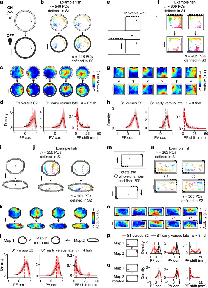
Fig. 4 PC activity can be stable despite environmental changes when path integration is uninterrupted. a, Schematic of the light/dark experiment (Methods). b, Change in distribution of telencephalic PCs with confined PFs (Methods). PCs defined in S1 or S2 are plotted separately (left and right, respectively) for an example animal. Each dot represents the COM of one cell’s PF, colour coded by its position in the chamber (top, S1; bottom, S2). c, Example spatial activity maps (one cell per column). d, Spatial activity map correlation (PF cor.), population vector correlation (PV cor.) and shift in PF location (PF shift; Methods) are shown from left to right. Comparisons between S1 and S2 (red) are plotted together with control comparisons between the early (first half) and late (second half) periods of S1 (black). Solid lines denote mean distributions across all fish, shaded regions denote s.d. across all fish and vertical dashed lines represent medians of averaged distributions (the same applies to all histograms in this figure). e, Schematic of landmark-removal experiment (Methods). f–h, Analysis of landmark-removal experiment; f,g,h correspond to b,c,d, respectively. i, Schematic of wall-morphing experiment (Methods). j–l, Analysis of wall-morphing experiment; j,k,l correspond to b,c,d, respectively. To facilitate comparisons in l, we represent the activity of both sessions in terms of the spatial bins of S1 (see Methods for non-rigid morphing of the S2 spatial activity map). m, Schematic of chamber-rotation experiment. Between sessions the entire chamber including the fish is rotated 180° relative to the microscope (Methods). n,o, Analysis of chamber-rotation experiment; n,o correspond to b,c, respectively. p, Summary of map changes in telencephalic PCs across the two sessions by direct comparison of maps in the microscope reference frame. q, Similar to l, but the comparison is made in the chamber reference frame by rotating the spatial activity maps (Methods). Statistical tests for individual animals are summarized in Extended Data Fig. 6a. Scale bars, 10 mm. Source Data
Fig. 4 PC activity can be stable despite environmental changes when path integration is uninterrupted. a, Schematic of the light/dark experiment (Methods). b, Change in distribution of telencephalic PCs with confined PFs (Methods). PCs defined in S1 or S2 are plotted separately (left and right, respectively) for an example animal. Each dot represents the COM of one cell’s PF, colour coded by its position in the chamber (top, S1; bottom, S2). c, Example spatial activity maps (one cell per column). d, Spatial activity map correlation (PF cor.), population vector correlation (PV cor.) and shift in PF location (PF shift; Methods) are shown from left to right. Comparisons between S1 and S2 (red) are plotted together with control comparisons between the early (first half) and late (second half) periods of S1 (black). Solid lines denote mean distributions across all fish, shaded regions denote s.d. across all fish and vertical dashed lines represent medians of averaged distributions (the same applies to all histograms in this figure). e, Schematic of landmark-removal experiment (Methods). f–h, Analysis of landmark-removal experiment; f,g,h correspond to b,c,d, respectively. i, Schematic of wall-morphing experiment (Methods). j–l, Analysis of wall-morphing experiment; j,k,l correspond to b,c,d, respectively. To facilitate comparisons in l, we represent the activity of both sessions in terms of the spatial bins of S1 (see Methods for non-rigid morphing of the S2 spatial activity map). m, Schematic of chamber-rotation experiment. Between sessions the entire chamber including the fish is rotated 180° relative to the microscope (Methods). n,o, Analysis of chamber-rotation experiment; n,o correspond to b,c, respectively. p, Summary of map changes in telencephalic PCs across the two sessions by direct comparison of maps in the microscope reference frame. q, Similar to l, but the comparison is made in the chamber reference frame by rotating the spatial activity maps (Methods). Statistical tests for individual animals are summarized in Extended Data Fig. 6a. Scale bars, 10 mm. Source DataCC BY · PubMed Central
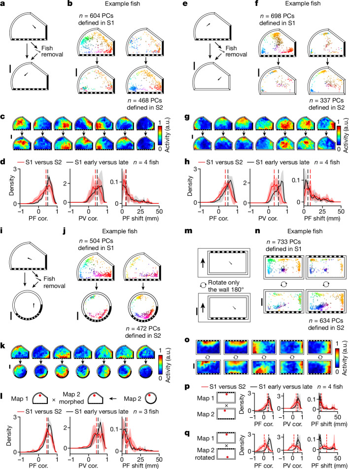
Fig. 5 Allothetic visual information contributes to PC activity. a, Schematic of the fish-removal experiment. The fish was removed from the chamber to break path integration between recording sessions performed in the same asymmetric chamber with landmarks (Methods). b–d, Analysis of fish-removal experiments as in Fig. 4b–d, with b,c,d representing the same analyses in both figures. For all histograms, solid lines indicate mean distributions across all fish, shaded regions indicate s.d. across all fish and vertical dashed lines indicate medians of averaged distributions. e, Schematic of the landmark-removal experiment with fish removal. Following the first recording session in an asymmetric chamber with landmarks, the fish was removed and transferred to a chamber with the same geometry but no landmarks for the second recording session (Methods). f–h, Analysis of landmark-removal experiment with fish removal; f,g,h correspond to Fig. 4b–d, respectively. i. Schematic of the wall-morphing experiment with fish removal. Following the first recording session in an asymmetric chamber with landmarks, the fish was removed and transferred to a chamber with the same landmarks but a different geometry for the second recording session (Methods). One out of three fish went in the reverse direction—it was transferred from the circular chamber to the asymmetric chamber. j–l, Analysis of wall-morphing experiment with fish removal as in Fig. 4j–l, respectively. m, Schematic of wall-rotation experiment without fish removal. In comparison to the experiment shown in Fig. 4m, here only the chamber wall, but not the fish, is rotated 180° relative to both the fish and microscope (Methods). n–q, Analysis of wall-rotation experiment as in Fig. 4n–q, respectively. The results of statistical tests for individual animals are summarized in Extended Data Fig. 6a. Scale bars, 10 mm. Source Data
Fig. 5 Allothetic visual information contributes to PC activity. a, Schematic of the fish-removal experiment. The fish was removed from the chamber to break path integration between recording sessions performed in the same asymmetric chamber with landmarks (Methods). b–d, Analysis of fish-removal experiments as in Fig. 4b–d, with b,c,d representing the same analyses in both figures. For all histograms, solid lines indicate mean distributions across all fish, shaded regions indicate s.d. across all fish and vertical dashed lines indicate medians of averaged distributions. e, Schematic of the landmark-removal experiment with fish removal. Following the first recording session in an asymmetric chamber with landmarks, the fish was removed and transferred to a chamber with the same geometry but no landmarks for the second recording session (Methods). f–h, Analysis of landmark-removal experiment with fish removal; f,g,h correspond to Fig. 4b–d, respectively. i. Schematic of the wall-morphing experiment with fish removal. Following the first recording session in an asymmetric chamber with landmarks, the fish was removed and transferred to a chamber with the same landmarks but a different geometry for the second recording session (Methods). One out of three fish went in the reverse direction—it was transferred from the circular chamber to the asymmetric chamber. j–l, Analysis of wall-morphing experiment with fish removal as in Fig. 4j–l, respectively. m, Schematic of wall-rotation experiment without fish removal. In comparison to the experiment shown in Fig. 4m, here only the chamber wall, but not the fish, is rotated 180° relative to both the fish and microscope (Methods). n–q, Analysis of wall-rotation experiment as in Fig. 4n–q, respectively. The results of statistical tests for individual animals are summarized in Extended Data Fig. 6a. Scale bars, 10 mm. Source DataCC BY · PubMed Central
Fig. 6 PCs exhibit representational flexibility across distinct environments. a, Schematic of the experiment combining landmark removal, wall morphing and fish removal. Following S1, the fish was removed and transferred to a chamber with a different geometry and no landmarks for S2 (Methods). b–d, Analysis of experiment performed as in Fig. 4j–l, respectively. d, For all histograms, solid lines indicate mean distributions across all fish, shaded regions indicate s.d. across all fish and vertical dashed lines indicate medians of averaged distributions. Results of statistical tests for individual animals are summarized in Extended Data Fig. 6a. e, We quantify the degree to which neighbourhood relationships between telencephalic PCs are maintained across sessions (‘neighbour retention %’; Methods). For each PC, neighbours are defined as cells with the highest PF correlation to the cell of interest, with a systematically varied inclusion threshold from the top 2% to the top 100%. Neighbour retention % is defined as the number of PCs that remain neighbours in S2 divided by the number of original neighbours in S1. The average neighbour retention % across PCs between S1 and S2 (solid red line) is plotted against the control comparison between the early and late stages of S1 (solid black line), as well as against comparisons with shuffled data (solid grey line). We also subdivided neurons into two groups based on the distance of each place field to the edge of the chamber in S1 (dashed lines represent distance to edge 3 mm or less, 233 ± 135 cells, mean ± s.d.; dotted lines represent distance to edge greater than 3 mm, 352 ± 171 cells, mean ± s.d.). Scale bars, 10 mm. Source Data
Fig. 6 PCs exhibit representational flexibility across distinct environments. a, Schematic of the experiment combining landmark removal, wall morphing and fish removal. Following S1, the fish was removed and transferred to a chamber with a different geometry and no landmarks for S2 (Methods). b–d, Analysis of experiment performed as in Fig. 4j–l, respectively. d, For all histograms, solid lines indicate mean distributions across all fish, shaded regions indicate s.d. across all fish and vertical dashed lines indicate medians of averaged distributions. Results of statistical tests for individual animals are summarized in Extended Data Fig. 6a. e, We quantify the degree to which neighbourhood relationships between telencephalic PCs are maintained across sessions (‘neighbour retention %’; Methods). For each PC, neighbours are defined as cells with the highest PF correlation to the cell of interest, with a systematically varied inclusion threshold from the top 2% to the top 100%. Neighbour retention % is defined as the number of PCs that remain neighbours in S2 divided by the number of original neighbours in S1. The average neighbour retention % across PCs between S1 and S2 (solid red line) is plotted against the control comparison between the early and late stages of S1 (solid black line), as well as against comparisons with shuffled data (solid grey line). We also subdivided neurons into two groups based on the distance of each place field to the edge of the chamber in S1 (dashed lines represent distance to edge 3 mm or less, 233 ± 135 cells, mean ± s.d.; dotted lines represent distance to edge greater than 3 mm, 352 ± 171 cells, mean ± s.d.). Scale bars, 10 mm. Source DataCC BY · PubMed Central
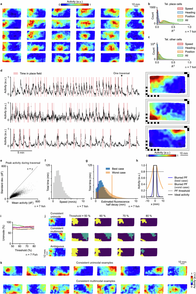
Extended Data Fig. 1 Place cell properties. a, Example spatial activity maps at different locations in the chamber. b, Modeling the relationship between activity and behavioral variables for telencephalic PCs. R² values of individual spatially tuned telencephalic cells after modeling their activity with ordinary least squares regression (OLS, Methods) using only the animal’s speed, heading, or two-dimensional position, as well as using all of them combined (n = 7 animals). c, Modeling the relationship between activity and behavioral variables for other cells in the telencephalon. d, Activity traces (left) and spatial activity maps (right) for three example PCs. The time that the fish spent inside the PF is marked in red. e, Statistics on the firing variability of PCs. One dot represents the mean and standard deviation of the peak activity across all traversals of one PC. A traversal is defined as a stay inside the PF that is interrupted only by departures shorter than 5 s. Data pooled across 7 animals. f, Distribution of swimming speed from the whole experiment from 7 animals, excluding quiescent time periods (swimming speed < 0.1 mm/s). g, Distribution of the estimated GCaMP6s fluorescence half decay distance in one linear dimension, based on the data from f, and assuming decay half-times of 0.56 s (10 Hz firing rate) and 1.21 s (80 Hz firing rate). Vertical lines indicate the mean - std. dev. for the best case and the mean + std. dev. for the worst case, based on the values of the distributions. h, Estimated actual PF blurring in one dimension based on an ideal PF with sharp edges (black line, −2.5 mm to 2.5 mm) and the best and worst cases of half decay distances shown in g (blue and orange lines). PF size is determined by the set of spatial bins with activity above 80% of the peak activity (with peak defined as 95th percentile) of the spatial activity map. Blurring to each side is 0.17 mm (best case) and 1.31 mm (worst case). i, Percentage of unimodal PCs as a function of the threshold for defining the firing field. j, Spatial activity maps (left) and thresholded firing fields (right) at different thresholds for an example neuron with consistently unimodal firing field (top), a neuron with consistently multimodal firing field (middle), and an ambiguous neuron (bottom) with unimodal or multimodal firing field depending on the choice of threshold between 50% and 80%. k. More examples of neurons that are consistently unimodal (top) or consistently multimodal (bottom) as firing field threshold is swept between 50% and 80%.
Extended Data Fig. 1 Place cell properties. a, Example spatial activity maps at different locations in the chamber. b, Modeling the relationship between activity and behavioral variables for telencephalic PCs. R² values of individual spatially tuned telencephalic cells after modeling their activity with ordinary least squares regression (OLS, Methods) using only the animal’s speed, heading, or two-dimensional position, as well as using all of them combined (n = 7 animals). c, Modeling the relationship between activity and behavioral variables for other cells in the telencephalon. d, Activity traces (left) and spatial activity maps (right) for three example PCs. The time that the fish spent inside the PF is marked in red. e, Statistics on the firing variability of PCs. One dot represents the mean and standard deviation of the peak activity across all traversals of one PC. A traversal is defined as a stay inside the PF that is interrupted only by departures shorter than 5 s. Data pooled across 7 animals. f, Distribution of swimming speed from the whole experiment from 7 animals, excluding quiescent time periods (swimming speed < 0.1 mm/s). g, Distribution of the estimated GCaMP6s fluorescence half decay distance in one linear dimension, based on the data from f, and assuming decay half-times of 0.56 s (10 Hz firing rate) and 1.21 s (80 Hz firing rate). Vertical lines indicate the mean - std. dev. for the best case and the mean + std. dev. for the worst case, based on the values of the distributions. h, Estimated actual PF blurring in one dimension based on an ideal PF with sharp edges (black line, −2.5 mm to 2.5 mm) and the best and worst cases of half decay distances shown in g (blue and orange lines). PF size is determined by the set of spatial bins with activity above 80% of the peak activity (with peak defined as 95th percentile) of the spatial activity map. Blurring to each side is 0.17 mm (best case) and 1.31 mm (worst case). i, Percentage of unimodal PCs as a function of the threshold for defining the firing field. j, Spatial activity maps (left) and thresholded firing fields (right) at different thresholds for an example neuron with consistently unimodal firing field (top), a neuron with consistently multimodal firing field (middle), and an ambiguous neuron (bottom) with unimodal or multimodal firing field depending on the choice of threshold between 50% and 80%. k. More examples of neurons that are consistently unimodal (top) or consistently multimodal (bottom) as firing field threshold is swept between 50% and 80%.CC BY · PubMed Central
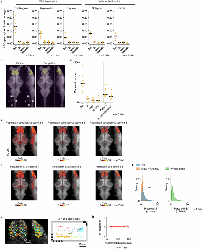
Extended Data Fig. 2 Anatomical analysis of place cells. a, Fraction of cells within each brain region that are classified as PCs, shown for five differently shaped behavioral chambers with or without landmarks: rectangle (Fig. 1a), asymmetric shape (Fig. 5a), square (Fig. 4e), octagon (Fig. 4i), and circle (Fig. 6a). b, Projections of telencephalic subdivisions: pallium and subpallium. Masks imported from the Z-Brain-Atlas. c, Number of PCs in each brain region. Each animal is shown individually (orange dots, n = 7 animals) along with the median across animals (black line). Tel., telencephalon; Mes., mesencephalon; Di., diencephalon; Rhomb., rhombencephalon. d, Anatomical distribution of cells that would be classified as PCs at different spatial specificity thresholds, based on a population specificity z-score ≥ 1 (left), ≥ 3 (middle), and ≥ 5 (right). Summation of 7 animals overlaid on a reference brain. The black bar indicates 50 μm. e, Anatomical distribution of cells that would be classified as PCs at different spatial information (SI) thresholds, based on a population SI z-score ≥ 1 (left), ≥ 3 (middle), and ≥ 5 (right). f, Comparison of SI for PCs found in the telencephalon and PCs found in the mesencephalon and rhombencephalon (left, n = 7 animals, p = 1.1 × 10−98, one-sided Mann–Whitney U test), as well as all PCs found in the whole brain (right, n = 7 animals). Since SI was calculated from calcium activity without attempting to convert to spikes/s, the SI values reported here are proportional to classic SI, measured in bits/s, but with an unspecified constant of proportionality. g, Anatomical distribution of PCs (left) colored by their PF locations (right). h, The relationship between anatomical distance and PF correlation. The solid line indicates the mean. The shaded region indicates the standard error of the mean. To avoid any potential caveat of imperfect cell merging along the dorsal-ventral axis, only cell pairs from the same horizontal plane are plotted. To avoid overestimating correlation due to shared measurement noise, adjacent cell pairs with NMF spatial footprints having any shared pixels are excluded (1.19% ± 0.54% of all cell pairs).
Extended Data Fig. 2 Anatomical analysis of place cells. a, Fraction of cells within each brain region that are classified as PCs, shown for five differently shaped behavioral chambers with or without landmarks: rectangle (Fig. 1a), asymmetric shape (Fig. 5a), square (Fig. 4e), octagon (Fig. 4i), and circle (Fig. 6a). b, Projections of telencephalic subdivisions: pallium and subpallium. Masks imported from the Z-Brain-Atlas. c, Number of PCs in each brain region. Each animal is shown individually (orange dots, n = 7 animals) along with the median across animals (black line). Tel., telencephalon; Mes., mesencephalon; Di., diencephalon; Rhomb., rhombencephalon. d, Anatomical distribution of cells that would be classified as PCs at different spatial specificity thresholds, based on a population specificity z-score ≥ 1 (left), ≥ 3 (middle), and ≥ 5 (right). Summation of 7 animals overlaid on a reference brain. The black bar indicates 50 μm. e, Anatomical distribution of cells that would be classified as PCs at different spatial information (SI) thresholds, based on a population SI z-score ≥ 1 (left), ≥ 3 (middle), and ≥ 5 (right). f, Comparison of SI for PCs found in the telencephalon and PCs found in the mesencephalon and rhombencephalon (left, n = 7 animals, p = 1.1 × 10−98, one-sided Mann–Whitney U test), as well as all PCs found in the whole brain (right, n = 7 animals). Since SI was calculated from calcium activity without attempting to convert to spikes/s, the SI values reported here are proportional to classic SI, measured in bits/s, but with an unspecified constant of proportionality. g, Anatomical distribution of PCs (left) colored by their PF locations (right). h, The relationship between anatomical distance and PF correlation. The solid line indicates the mean. The shaded region indicates the standard error of the mean. To avoid any potential caveat of imperfect cell merging along the dorsal-ventral axis, only cell pairs from the same horizontal plane are plotted. To avoid overestimating correlation due to shared measurement noise, adjacent cell pairs with NMF spatial footprints having any shared pixels are excluded (1.19% ± 0.54% of all cell pairs).CC BY · PubMed Central
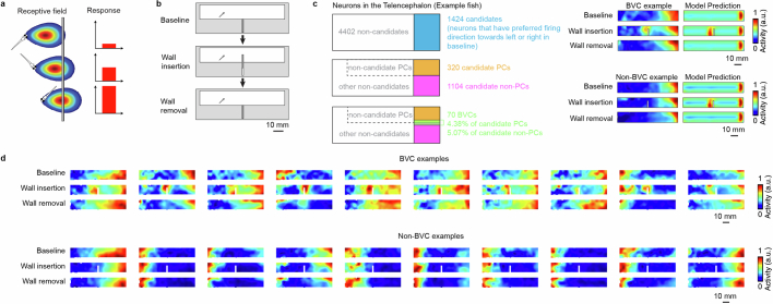
Extended Data Fig. 3 Boundary vector cell analysis. a, Schematic of the boundary vector cell (BVC) model, adapted from Lever et al.33. A BVC reaches the highest firing rate when the animal is at its preferred firing orientation and distance to the wall. b, Schematic of the experiment to test for BVCs in the larval zebrafish brain (Methods). A wall hidden in the middle of the rectangular chamber is inserted between the 1st session (baseline) and the 2nd session of the experiment. Then the wall is removed again for the recording of the 3rd session of the experiment. The BVC model predicts that a BVC with a preferred horizontal firing orientation would duplicate its firing field when a new wall is inserted. c, Procedure for identification of boundary vector cells. First, we identified suitable candidate cells in the telencephalon with PFs parallel to the inserted wall (which could be PCs or non-PCs, left). We then fit the BVC model to the spatial activity maps of these candidate cells in session 1 and used the fitted model to generate predicted activity maps across sessions (with or without wall insertion). We compare the actual spatial activity maps (left) and the corresponding map predicted by the BVC model (right) to evaluate whether each cell is consistent with the BVC model. For each telencephalic candidate cell, the model is fit to the baseline (1st session) and then used to predict the spatial activity map for the case of wall insertion or removal (2nd and 3rd sessions, Methods). Top right shows an example neuron that is consistent with the BVC model prediction. Bottom right shows an example of a neuron that does not follow the BVC model prediction. d, Additional examples of neurons that follow and do not follow the BVC model prediction.
Extended Data Fig. 3 Boundary vector cell analysis. a, Schematic of the boundary vector cell (BVC) model, adapted from Lever et al.33. A BVC reaches the highest firing rate when the animal is at its preferred firing orientation and distance to the wall. b, Schematic of the experiment to test for BVCs in the larval zebrafish brain (Methods). A wall hidden in the middle of the rectangular chamber is inserted between the 1st session (baseline) and the 2nd session of the experiment. Then the wall is removed again for the recording of the 3rd session of the experiment. The BVC model predicts that a BVC with a preferred horizontal firing orientation would duplicate its firing field when a new wall is inserted. c, Procedure for identification of boundary vector cells. First, we identified suitable candidate cells in the telencephalon with PFs parallel to the inserted wall (which could be PCs or non-PCs, left). We then fit the BVC model to the spatial activity maps of these candidate cells in session 1 and used the fitted model to generate predicted activity maps across sessions (with or without wall insertion). We compare the actual spatial activity maps (left) and the corresponding map predicted by the BVC model (right) to evaluate whether each cell is consistent with the BVC model. For each telencephalic candidate cell, the model is fit to the baseline (1st session) and then used to predict the spatial activity map for the case of wall insertion or removal (2nd and 3rd sessions, Methods). Top right shows an example neuron that is consistent with the BVC model prediction. Bottom right shows an example of a neuron that does not follow the BVC model prediction. d, Additional examples of neurons that follow and do not follow the BVC model prediction.CC BY · PubMed Central
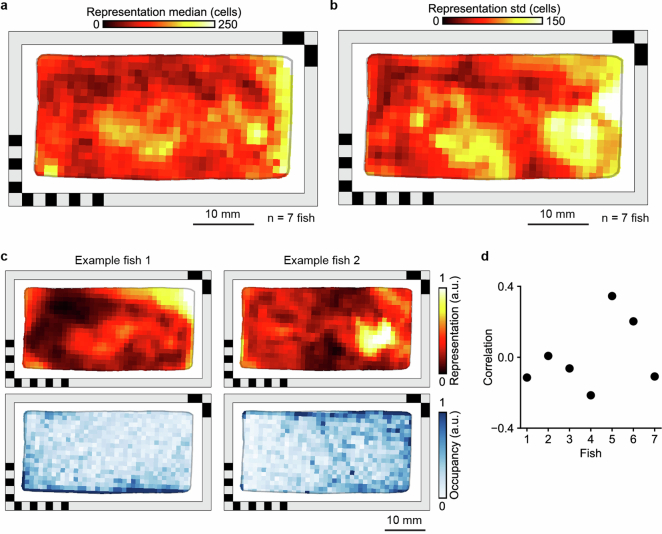
Extended Data Fig. 4 Spatial representation and occupancy. a, Distribution of telencephalic PFs encoding different locations in the behavioral arena (same as Fig. 2a, n = 7 animals, median across animals is shown). To quantify the density of PFs across space, each spatial activity map was binarized. b, same as a, but showing the standard deviation of spatial representation across the 7 animals. c, Spatial representation (top) and spatial occupancy (bottom) for two example fish. Representation and occupancy are both normalized. d, Correlation between spatial representation and occupancy for 7 different animals.
Extended Data Fig. 4 Spatial representation and occupancy. a, Distribution of telencephalic PFs encoding different locations in the behavioral arena (same as Fig. 2a, n = 7 animals, median across animals is shown). To quantify the density of PFs across space, each spatial activity map was binarized. b, same as a, but showing the standard deviation of spatial representation across the 7 animals. c, Spatial representation (top) and spatial occupancy (bottom) for two example fish. Representation and occupancy are both normalized. d, Correlation between spatial representation and occupancy for 7 different animals.CC BY · PubMed Central
Extended Data Fig. 5 Additional quantification of decoder error. a, Distribution of decoder error for 7 animals. Vertical lines indicate the median error (black line), the behavior-informed baseline (15.08 mm, dashed line), and the accessible length of the chamber’s long axis (47 mm, dotted line). b, Replication of Fig. 2f but excluding from training the 2 min before and 2 min after the 1 min used for decoding (Methods). The solid line indicates the mean, and the shaded region indicates the standard deviation (the same applies to c). c, Decoder error as a function of timing shift between neural activity and animal position.
Extended Data Fig. 5 Additional quantification of decoder error. a, Distribution of decoder error for 7 animals. Vertical lines indicate the median error (black line), the behavior-informed baseline (15.08 mm, dashed line), and the accessible length of the chamber’s long axis (47 mm, dotted line). b, Replication of Fig. 2f but excluding from training the 2 min before and 2 min after the 1 min used for decoding (Methods). The solid line indicates the mean, and the shaded region indicates the standard deviation (the same applies to c). c, Decoder error as a function of timing shift between neural activity and animal position.CC BY · PubMed Central
Extended Data Fig. 6 Summary of spatial activity map changes of telencephalic place cells under different environmental manipulations. a, The median of PF correlation (top), PV correlation (middle), and PF shift (bottom) for individual fish. Gray dots are comparisons between the early (1st half) and late (2nd half) stages of the 1st session. The red dots are comparisons made between the 1st session and the 2nd session. Experiments from Figs. 4–6 are represented on the horizontal axis: chamber rotation (Fig. 4m), landmark removal (Fig. 4e), wall morphing (Fig. 4i), wall rotation (Fig. 5m), fish removal with no change in the chamber (Fig. 5a), landmark removal with fish removal (Fig. 5e), wall morphing with fish removal (Fig. 5i), and wall morphing with landmark removal and fish removal (Fig. 6a). Data from the same fish are connected by gray lines. The results of statistical tests are marked for each fish separately (one-sided Wilcoxon signed-rank test, *** for p < 10−5, ** for p < 0.001, * for p < 0.01, n.s. for p ≥ 0.01, see Supplementary Table 1 for exact p-values). b, The relationship between PF overlap and PF correlation for different experiments. Each dot represents a PC. PF overlap is defined as the intersection over union of its PFs in the two sessions or between the early and late half of session 1 (as control). Orange dots denote cells with significant PF correlation (one-sided shuffle test, p < 0.05). Briefly, to test the significance of the PF correlation, we circularly permuted (~ 1000 times, corresponding to the number of bins in the map) the observed spatial activity map of session 2 (or the 2nd half of session 1 in controls), and recalculated the PF correlation across sessions for each permutation to construct the null distribution for a one-sided shuffle test. c, The dropout rates of PCs for individual fish (gray, within session control; red, cross-session comparison, as defined in a). A dropout cell is defined as a cell that does not retain significant PF correlation between sessions and is only classified as a PC in the first but not second session.
Extended Data Fig. 6 Summary of spatial activity map changes of telencephalic place cells under different environmental manipulations. a, The median of PF correlation (top), PV correlation (middle), and PF shift (bottom) for individual fish. Gray dots are comparisons between the early (1st half) and late (2nd half) stages of the 1st session. The red dots are comparisons made between the 1st session and the 2nd session. Experiments from Figs. 4–6 are represented on the horizontal axis: chamber rotation (Fig. 4m), landmark removal (Fig. 4e), wall morphing (Fig. 4i), wall rotation (Fig. 5m), fish removal with no change in the chamber (Fig. 5a), landmark removal with fish removal (Fig. 5e), wall morphing with fish removal (Fig. 5i), and wall morphing with landmark removal and fish removal (Fig. 6a). Data from the same fish are connected by gray lines. The results of statistical tests are marked for each fish separately (one-sided Wilcoxon signed-rank test, *** for p < 10−5, ** for p < 0.001, * for p < 0.01, n.s. for p ≥ 0.01, see Supplementary Table 1 for exact p-values). b, The relationship between PF overlap and PF correlation for different experiments. Each dot represents a PC. PF overlap is defined as the intersection over union of its PFs in the two sessions or between the early and late half of session 1 (as control). Orange dots denote cells with significant PF correlation (one-sided shuffle test, p < 0.05). Briefly, to test the significance of the PF correlation, we circularly permuted (~ 1000 times, corresponding to the number of bins in the map) the observed spatial activity map of session 2 (or the 2nd half of session 1 in controls), and recalculated the PF correlation across sessions for each permutation to construct the null distribution for a one-sided shuffle test. c, The dropout rates of PCs for individual fish (gray, within session control; red, cross-session comparison, as defined in a). A dropout cell is defined as a cell that does not retain significant PF correlation between sessions and is only classified as a PC in the first but not second session.CC BY · PubMed Central
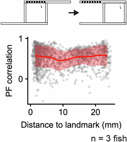
Extended Data Fig. 7 Place field correlation versus environmental features. Top, schematic of landmark removal experiment (Fig. 4e). Bottom, PF correlation between recording sessions in the landmark removal experiment as a function of the distance of the PF (represented by its COM) to the landmark. Red line indicates mean values after binning the data (n = 10 bins), red shaded region indicates standard deviation within bins.
Extended Data Fig. 7 Place field correlation versus environmental features. Top, schematic of landmark removal experiment (Fig. 4e). Bottom, PF correlation between recording sessions in the landmark removal experiment as a function of the distance of the PF (represented by its COM) to the landmark. Red line indicates mean values after binning the data (n = 10 bins), red shaded region indicates standard deviation within bins.CC BY · PubMed Central
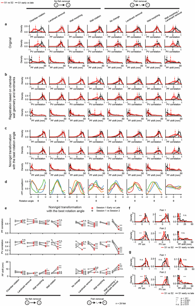
Extended Data Fig. 8 Additional quantification of map comparisons. a, Summary of the changes in telencephalic PCs by directly comparing the maps across two sessions in the microscope reference frame. Experiments from Fig. 4 and Fig. 5 are represented on the horizontal axis: chamber rotation (Fig. 4m), landmark removal (Fig. 4e), wall morphing (Fig. 4i), wall rotation (Fig. 5m), fish removal with no change in the chamber (Fig. 5a), landmark removal with fish removal (Fig. 5e), wall morphing with fish removal (Fig. 5i), and wall morphing with landmark removal and fish removal (Fig. 6a). From top to bottom are place field correlation (PF correlation), population vector correlation (PV correlation), and the shift in the place field location (PF shift, Methods). The union of telencephalic PCs from both sessions was used. The comparison between the 1st and the 2nd sessions (red) is plotted against a reference comparison between the early (1st half) and late (2nd half) stages of the 1st session (black). Solid lines are the mean distributions across all fish, and the shaded region indicates the standard deviation across all fish. Vertical dashed lines are the medians of the averaged distributions. b, similar to a but after registering the maps from the 2nd session to the 1st session with reference to the chamber wall geometry and landmarks (Methods). c, similar to b but the transformation is done by finding the rotation of the reference anchor points that maximizes the mean PF correlation after registration (Methods). d, The mean PF correlation as a function of the anchor rotation angle used in the nonrigid transformation, for different experiments (Methods). e, Summary of changes in the spatial activity maps of telencephalic PCs under different environmental manipulations after applying the nonrigid transformation with the best rotation angle. The median of PF correlation, PV correlation, and PF shift are plotted for each fish. Red dots are comparisons made between the 1st session and the 2nd session. Gray dots are reference comparisons made between the early (1st half) and late (2nd half) stages of the 1st session (also after nonrigid transformation with the best rotation angle). The results of statistical tests are marked for each fish separately (one-sided Wilcoxon signed-rank test, *** for p < 10−5, ** for p < 0.001, * for p < 0.01, n.s. for p ≥ 0.01). See Supplementary Table 1 for exact p-values. f, Analysis of fish removal experiment as in Fig. 5d, but only for individual fish where the olfactory cues were cleaned thoroughly before each recording session with soap and isopropanol. The results of statistical tests for different measures against a control comparison between the early (1st half) and late (2nd half) period of the 1st session are shown for each fish (one-sided Wilcoxon signed-rank test, same for Extended Data Fig. 8g, fish 1 and fish 2 corresponds to fish 1 and fish 2 in Supplementary Table 1). g, Analysis of fish removal experiment as in Fig. 5d, but only for individual fish where the bottom was rotated without cleaning to scramble any potential olfactory cues (fish 1 and fish 2 correspond to fish 3 and fish 4 in Supplementary Table 1). See Supplementary Table 1 for exact p-values.
Extended Data Fig. 8 Additional quantification of map comparisons. a, Summary of the changes in telencephalic PCs by directly comparing the maps across two sessions in the microscope reference frame. Experiments from Fig. 4 and Fig. 5 are represented on the horizontal axis: chamber rotation (Fig. 4m), landmark removal (Fig. 4e), wall morphing (Fig. 4i), wall rotation (Fig. 5m), fish removal with no change in the chamber (Fig. 5a), landmark removal with fish removal (Fig. 5e), wall morphing with fish removal (Fig. 5i), and wall morphing with landmark removal and fish removal (Fig. 6a). From top to bottom are place field correlation (PF correlation), population vector correlation (PV correlation), and the shift in the place field location (PF shift, Methods). The union of telencephalic PCs from both sessions was used. The comparison between the 1st and the 2nd sessions (red) is plotted against a reference comparison between the early (1st half) and late (2nd half) stages of the 1st session (black). Solid lines are the mean distributions across all fish, and the shaded region indicates the standard deviation across all fish. Vertical dashed lines are the medians of the averaged distributions. b, similar to a but after registering the maps from the 2nd session to the 1st session with reference to the chamber wall geometry and landmarks (Methods). c, similar to b but the transformation is done by finding the rotation of the reference anchor points that maximizes the mean PF correlation after registration (Methods). d, The mean PF correlation as a function of the anchor rotation angle used in the nonrigid transformation, for different experiments (Methods). e, Summary of changes in the spatial activity maps of telencephalic PCs under different environmental manipulations after applying the nonrigid transformation with the best rotation angle. The median of PF correlation, PV correlation, and PF shift are plotted for each fish. Red dots are comparisons made between the 1st session and the 2nd session. Gray dots are reference comparisons made between the early (1st half) and late (2nd half) stages of the 1st session (also after nonrigid transformation with the best rotation angle). The results of statistical tests are marked for each fish separately (one-sided Wilcoxon signed-rank test, *** for p < 10−5, ** for p < 0.001, * for p < 0.01, n.s. for p ≥ 0.01). See Supplementary Table 1 for exact p-values. f, Analysis of fish removal experiment as in Fig. 5d, but only for individual fish where the olfactory cues were cleaned thoroughly before each recording session with soap and isopropanol. The results of statistical tests for different measures against a control comparison between the early (1st half) and late (2nd half) period of the 1st session are shown for each fish (one-sided Wilcoxon signed-rank test, same for Extended Data Fig. 8g, fish 1 and fish 2 corresponds to fish 1 and fish 2 in Supplementary Table 1). g, Analysis of fish removal experiment as in Fig. 5d, but only for individual fish where the bottom was rotated without cleaning to scramble any potential olfactory cues (fish 1 and fish 2 correspond to fish 3 and fish 4 in Supplementary Table 1). See Supplementary Table 1 for exact p-values.CC BY · PubMed Central
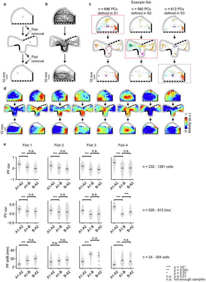
Extended Data Fig. 9 ABA experiment. a, Schematic of ABA experiment. After the 1st recording session in an asymmetric chamber with landmarks, the fish was removed and transferred into a chamber with a distinct arrangement of geometric features and landmarks for the 2nd recording session. For the 3rd recording session, the fish was removed and transferred back to the chamber that was used in the 1st recording session (Methods). b, Example animal trajectories in each session. c, Change in the distribution of telencephalic PCs with confined PFs, similar to Fig. 4b. Here, the distributions are plotted separately for 1st session (top), 2nd session (middle), and 3rd session (bottom) for an example animal. Red boxes indicate the session where telencephalic PCs were defined in each column. d, Example spatial activity maps as Fig. 4c. e, Summary of the changes in telencephalic PCs across the 1st and 2nd session, the 2nd and 3rd session, and the 1st and 3rd session. Similar to Fig. 4d, PF cor., PV cor., and PF shift were calculated for 4 fish. Each distribution uses the union of telencephalic PCs from the two sessions being compared. Grey shaded regions show the distribution of each measurement, and black horizontal bars indicate medians. Each column is one fish. The results of statistical tests are marked on top of the distributions being compared (one-sided Mann–Whitney U test, *** for p < 10−5, ** for p < 0.001, * for p < 0.01, n.s. for p ≥ 0.01, n.a. for not enough samples). The range of sample sizes are provided on the right of each metric. See Supplementary Table 1 for exact p-values and exact sample sizes.
Extended Data Fig. 9 ABA experiment. a, Schematic of ABA experiment. After the 1st recording session in an asymmetric chamber with landmarks, the fish was removed and transferred into a chamber with a distinct arrangement of geometric features and landmarks for the 2nd recording session. For the 3rd recording session, the fish was removed and transferred back to the chamber that was used in the 1st recording session (Methods). b, Example animal trajectories in each session. c, Change in the distribution of telencephalic PCs with confined PFs, similar to Fig. 4b. Here, the distributions are plotted separately for 1st session (top), 2nd session (middle), and 3rd session (bottom) for an example animal. Red boxes indicate the session where telencephalic PCs were defined in each column. d, Example spatial activity maps as Fig. 4c. e, Summary of the changes in telencephalic PCs across the 1st and 2nd session, the 2nd and 3rd session, and the 1st and 3rd session. Similar to Fig. 4d, PF cor., PV cor., and PF shift were calculated for 4 fish. Each distribution uses the union of telencephalic PCs from the two sessions being compared. Grey shaded regions show the distribution of each measurement, and black horizontal bars indicate medians. Each column is one fish. The results of statistical tests are marked on top of the distributions being compared (one-sided Mann–Whitney U test, *** for p < 10−5, ** for p < 0.001, * for p < 0.01, n.s. for p ≥ 0.01, n.a. for not enough samples). The range of sample sizes are provided on the right of each metric. See Supplementary Table 1 for exact p-values and exact sample sizes.CC BY · PubMed Central
Extended Data Fig. 10 Weakly coherent place field rotations during remapping. The increase in the median PF correlation (left), PV correlation (middle), and PF shift (right) are shown for 3 experiments: wall morphing without fish removal (Fig. 4i), wall morphing with fish removal (Fig. 5i), and wall morphing with landmark removal and fish removal (Fig. 6a). Blue dots show the comparison of session 1 and session 2 after registration of session 2 maps based on session 1 wall geometry and landmarks. Red dots show the comparison of session 1 and session 2 after registering session 2 maps to session 1 maps using the nonrigid transformation with the best rotation angle. Data from the same fish are connected by gray lines. The observed improvement in PF correlation from map rotation was evaluated by a non-parametric shuffle test (Methods), applied to each fish individually: wall morphing without fish removal (1/4 fish, p < 10−5, 3/4 fish, p ≥ 0.01), wall morphing with fish removal (1/3 fish, p < 10−5, 2/3 fish, p ≥ 0.01), and wall morphing with landmark removal and fish removal (2/4 fish, p < 10−5, 1/4 fish, p < 0.01, 1/4 fish, p ≥ 0.01). See Supplementary Table 1 for exact p-values.
Extended Data Fig. 10 Weakly coherent place field rotations during remapping. The increase in the median PF correlation (left), PV correlation (middle), and PF shift (right) are shown for 3 experiments: wall morphing without fish removal (Fig. 4i), wall morphing with fish removal (Fig. 5i), and wall morphing with landmark removal and fish removal (Fig. 6a). Blue dots show the comparison of session 1 and session 2 after registration of session 2 maps based on session 1 wall geometry and landmarks. Red dots show the comparison of session 1 and session 2 after registering session 2 maps to session 1 maps using the nonrigid transformation with the best rotation angle. Data from the same fish are connected by gray lines. The observed improvement in PF correlation from map rotation was evaluated by a non-parametric shuffle test (Methods), applied to each fish individually: wall morphing without fish removal (1/4 fish, p < 10−5, 3/4 fish, p ≥ 0.01), wall morphing with fish removal (1/3 fish, p < 10−5, 2/3 fish, p ≥ 0.01), and wall morphing with landmark removal and fish removal (2/4 fish, p < 10−5, 1/4 fish, p < 0.01, 1/4 fish, p ≥ 0.01). See Supplementary Table 1 for exact p-values.CC BY · PubMed Central

Verification

Claims the paper makes

15 Valid · 0 Not valid · 5 Not checked · 97 Own results and interpretations

51 more claims

Create a free account to see all 117 claims and to verify the 3 references still open.

See all claims — free account
  • Probably not a substantial claim. 31
  • It may state two separate claims as one. 35
  • The quote only partly states this claim. 1

Create a free account to see these claims.

Citations

Cites

Show all 55 references

Research works printed but not linked: 1

  1. Skaggs, W. E., Mcnaughton, B. L., Gothard, K. M. & Markus, E. J. Information theoretic approach to deciphering the hippocampal code. In Advances in Neural Information Processing System 5 (eds. Hanson, S. J., Cowan, J. D. & Giles, C. J.) 1030–1037 (Morgan Kaufmann, 1993) .

Cited by

See all 38

Metadata

Authors
Yang, C., Mammen, L., Kim, B., Li, M., Robson, D. N., & Li, J. M.
Affiliations
  • Max Planck Institute for Biological Cybernetics (DE)
  • Cornell University (US)
  • Chinese Academy of Sciences (CN)
Corresponding author
  • Robson, Drew N.
  • Li, Jennifer M.
Venue
Nature
Published
2024-08-28
Volume
634
Issue
8033
Pages
397-406
ISSN
  • 0028-0836 (ISSN-L)
  • 1476-4687
OpenAlex
W4401947288
Cited by
38
References
55
Citations by year
2026: 18 · 2025: 12 · 2024: 7
FWCI
8.96
Type
journal article
Language
en
Open access
Licence
Locations
  • Nature (publishedVersion, cc-by)
  • PubMed Central (publishedVersion, cc-by)
  • PubMed (publishedVersion)
  • RePEc: Research Papers in Economics (submittedVersion)
Topics
  • Life Sciences › Neuroscience › Cognitive Neuroscience › Memory and Neural Mechanisms
  • Life Sciences › Biochemistry, Genetics and Molecular Biology › Cell Biology › Zebrafish Biomedical Research Applications
  • Life Sciences › Neuroscience › Cognitive Neuroscience › Neural dynamics and brain function
Keywords
place cells, spatial representation, spatial learning, population coding, spatial maps, spatial cognition, zebrafish larvae, neural decoding
MeSH terms
Animals, Calcium, Cues, Larva, Microscopy, Neurons, Swimming, Telencephalon, Zebrafish, Spatial Learning

About these checks

Registry, retraction, Cites and statistics results are computed, not judged, with one exception: a printed reference that no index lists is read once by a model before it counts as a citation error. Claims are extracted by a model and kept only when their quote appears verbatim in the text; each cited source is then checked, with a model’s help, for whether it says what the claim relies on. Those verdicts can be wrong — read the claim’s quote and the cited source before relying on one.

The claim verdicts this report counts are experimental: their accuracy is not yet measured.

A language model drew the claims from the paper on 2026-10-10, under version 3 of the claim definition (model deepseek-v4.1-flash, prompt extract-v3).

A second model labelled each claim on 2026-10-10 (model jev-1.13-20260917, definition revision gold-guideline-v0.2).

Cited sources are checked with a language model’s help (gpt-6-sol).

Statistics and arithmetic are recomputed, not judged.

Confidence bands are shown only for fields calibrated on our annotated test set. None is calibrated yet, so no band is shown.

What counts as a claim ›How we measure confidence ›How we check this ›

Are you an author, or do you see a problem with this page? Request a review

How to cite

Cite CoChat for the checks on this page, and the paper for its own findings.

This page
CoChat. (2026). Citation check: A population code for spatial representation in the zebrafish telencephalon. https://app.cochat.ai/papers/10.1038/s41586-024-07867-2
The paper
Yang, C., Mammen, L., Kim, B., Li, M., Robson, D. N., & Li, J. M. (2024). A population code for spatial representation in the zebrafish telencephalon. Nature. https://doi.org/10.1038/s41586-024-07867-2

Data sources

Bibliographic data: Semantic Scholar, OpenAlex, Crossref.

Contains information from the Semantic Scholar Academic Graph Datasets, made available under the ODC Attribution License (ODC-BY 1.0).

Semantic Scholar’s data is described in: Kinney, R., et al. (2023). The Semantic Scholar Open Data Platform. arXiv:2301.10140.