

The DOI matches its Crossref record; 63 of the 63 references it cites were found in a registry or an index; 25 of the 56 sources its claims cite were checked for support.
A deep-learning framework reveals whole-body perturbations at cell level
Open accessAbstract
Many diseases, including obesity, have systemic effects that perturb multiple organ systems throughout the body 1,2 . However, tools for comprehensive, high-resolution analysis of disease-associated changes at the whole-body scale have been lacking. Here we developed MouseMapper, a suite of foundation-model-based deep-learning algorithms enabling multi-system analysis of disease across the entire mouse body. MouseMapper enables whole-body quantitative analysis of nerves and immune cells, resolving fine axonal branches and immune-cell clusters while automatically segmenting 31 organs and tissues. We used MouseMapper to study diet-induced obesity, and identified structural alterations of the infraorbital branch of the trigeminal ganglia. This structural impairment in infraorbital nerves was associated with functional sensory deficits in whisker sensing. Furthermore, we identified proteomic changes in the trigeminal ganglion affecting axon remodelling and complement pathways both in mice and humans. MouseMapper also generated detailed three-dimensional inflammation maps by characterizing immune cell cluster compositions across tissues. The MouseMapper framework demonstrates robust generalizability across different imaging resolutions and datasets. Our study provides a powerful, scalable approach for identifying and quantifying systemic pathologies, bridging molecular insights from animal models to human conditions.
Overview
CoChat Summary
TL;DR
The authors present MouseMapper, a foundation-model-based deep-learning framework that segments nerves, immune cells, and 31 organs/tissues across whole mouse bodies. Applying it to diet-induced obesity reveals reduced nerve density and infraorbital nerve structural changes linked to whisker sensory deficits, plus conserved trigeminal ganglion proteomic alterations in mice and humans.
Key findings
- MouseMapper automatically segments 31 organs and tissues, far exceeding previous methods such as AIMOS (six organs), and its Nerve-Module achieved a voxel Dice score of 0.7494, with cross-dataset Dice scores of 0.6916–0.7143 across different labelling strategies and resolutions.
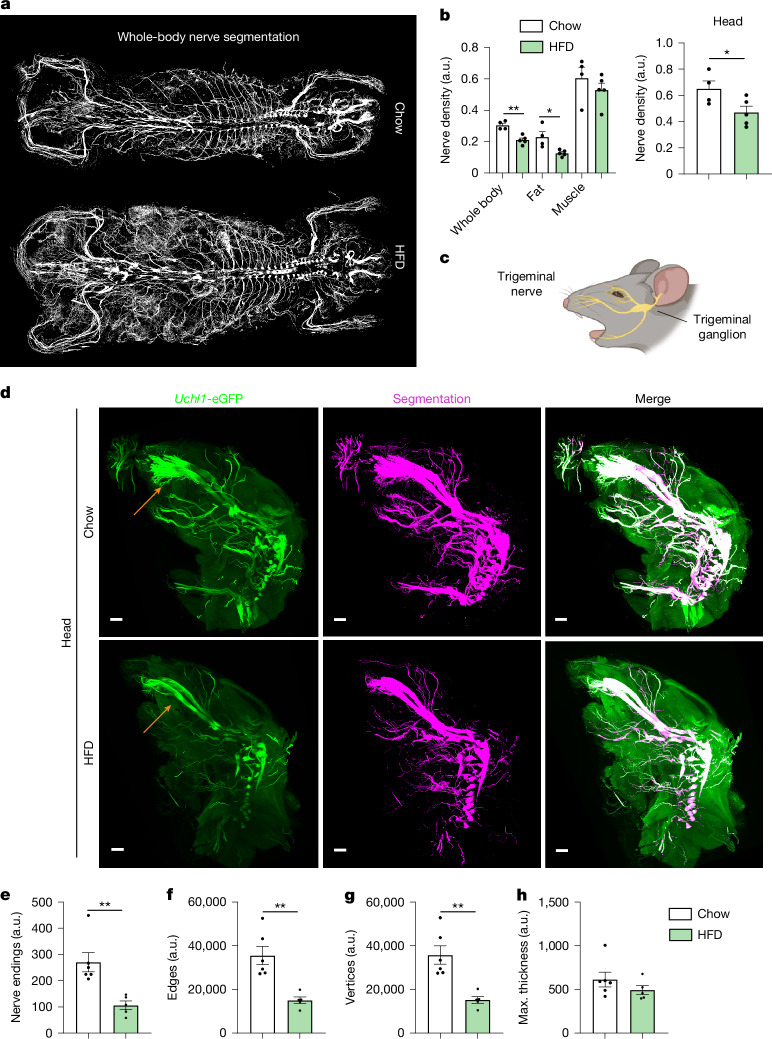
- In high-fat-diet-fed obese mice, whole-body nerve density decreased, including in adipose tissue and limbs; infraorbital nerve endings, edges, and vertices were reduced by 60.7%, 57.8%, and 57.6%, respectively, while nerve thickness was similar, and obese mice showed diminished whisker-stimulation responses.
- Trigeminal ganglion proteomics identified more than 6,000 proteins per sample, with 230 differentially regulated proteins (67 upregulated, 163 downregulated) in HFD-fed mice; pathways included actin cytoskeleton, RHO GTPase effectors, axon guidance, complement/coagulation, ERBB signalling, and sphingolipid signalling.
- Human post-mortem trigeminal ganglia from lean (BMI < 25) versus obese (BMI > 30) individuals showed conserved proteomic changes in axon guidance, neurodegeneration, and actin cytoskeleton regulation; the Immune-Module achieved voxel Dice 0.7878, outperforming existing methods (0.2140–0.5468).
Methods
- MouseMapper is an ensemble of three modules: Nerve-Module, Immune-Module, and Tissue-Module, built by fine-tuning the VesselFM 3D foundation model with supervised VR annotations and sliding-window inference on whole-body light-sheet fluorescence microscopy datasets.
- Male Uchl1-eGFP and Cd68-eGFP mice were fed chow or a 60% fat high-fat diet for 16–18 weeks; whole bodies were cleared with vDISCO or WildDISCO and imaged with ×1.1 (NA 0.1) or ×4 (NA 0.35) objectives. Human trigeminal ganglia were collected post-mortem from lean and obese body donors.
- Analyses included Dice-based segmentation benchmarking, connected-component and graph extraction for nerve morphology, Cd68+ cluster-size quantification, and mass-spectrometry-based spatial proteomics with pathway enrichment.
Limitations
- The paper states that whole-body light-sheet resolution limits resolving the smallest parenchymal nerve fibres and subcellular structures; the standard ×1.1 configuration has lateral resolution around 5.9 µm and cannot fully resolve thin axons, while the ×4 configuration (1.62 µm lateral resolution) increases data volumes up to 50 TB per mouse.
- The paper states that full generalizability across disparate imaging modalities is not yet attainable, and MouseMapper may require additional fine-tuning for optimal performance on new datasets; Uchl1-eGFP mice do not tag endogenous UCHL1, and antibody labelling was less homogeneous in obese mice.
- The paper states that no statistical method was used to predetermine sample size, and unless stated otherwise investigators were not blinded during experiments or data analysis; the text also makes evident that mouse experiments used male mice only.
Model-written summary. Check it against the paper before relying on it.
Integrity signals
Registry
Cites
Statistics
Figures




Verification
Claims the paper makes
10 Valid · 1 Not valid · 16 Not checked · 135 Own results and interpretations
The cited sources support only part of this claim — read each source’s verdict below.
In the paper
“However, tools for comprehensive, high-resolution analysis of disease-associated changes at the whole-body scale have been lacking.”
- Also stated in: § Main · plain
“However, tools to study cellular and molecular perturbations at the whole-body scale have been lacking, limiting our ability to understand their broad impacts.”
§ A deep-learning framework reveals whole-body perturbations at cell level > Abstract
What the sources say
- Supportedcites [6] Pan, C. et al. Deep learning reveals cancer metastasis and therapeutic antibody targeting in the entire body. Cell 179, 1661–1676 (2019). source
The INTRODUCTION of our copy states that efforts toward comprehensive, unbiased detection of disseminated tumor cells and tumor-targeting drugs within the entire body 'have been hampered by the lack of 1) imaging technologies to reliably detect all individual metastases and disseminating tumor cells in mouse bodies, and 2) algorithms to quickly and accurately quantify large-scale imaging data'. The DISCUSSION and its subsection on DeepMACT detection reinforce this, noting that established modalities (MRI, CT, bioluminescence) typically resolve only structures larger than 75 um and cannot detect smaller micrometastases. This matches the citing sentence's assertion that tools for comprehensive, high-resolution whole-body analysis of disease-associated changes were lacking. (LLM, conf=0.90)
- Partly supportedcites [7] Kaltenecker, D. et al. Virtual reality-empowered deep-learning analysis of brain cells. Nat. Methods https://doi.org/10.1038/s41592-024-02245-2 (2024). sourceExperimental — accuracy not yet measured
Our copy states a tooling gap, but bounded to the whole-brain: the Main section says unbiased single-cell quantification methods are essential yet 'current automated methods for cell detection and registration to the Allen Mouse Brain Atlas are difficult to apply consistently to three-dimensional (3D) whole-brain datasets', and the Discussion adds that only a subset of prior pipelines were released in a usable package — with disease relevance shown via cancer-associated cachexia brain activity. What it does not support is the claim's 'whole-body scale': the same Main passage says tissue clearing and fluorescent imaging 'allow unbiased protein expression analysis up to the whole-organism scale', and DELiVR itself is a whole-brain tool (Abstract). So the 'high-resolution/comprehensive analysis of disease-associated changes ... lacking' part is in the source at brain-wide scope, while the extension to whole-body is not. (LLM, conf=0.72)
- Partly supportedcites [8] Renier, N. et al. Mapping of brain activity by automated volume analysis of immediate early genes. Cell 165, 1789–1802 (2016). sourceExperimental — accuracy not yet measured
The Abstract (p. 1) states that precise detection, localization and quantification of the activity of all neurons across the entire brain, needed to understand neural processing in physiological and pathological states, 'has not to date been achieved in the mammalian brain', and the Discussion (p. ~13) likewise flags time and low throughput as major hurdles for unbiased IEG screens — this supports a gap in comprehensive, cellular-resolution mapping tools covering the whole brain, with pathological (disease-related) states as one motivation. What the source does NOT support is the claim's 'whole-body scale': our copy frames the limitation strictly at brain-wide scale (a 7 x 7 x 6 mm region of the mouse brain, atlas registration to the Allen mouse brain), and only speculates that iDISCO+/ClearMap 'could easily be used to map objects in other adult tissues or embryos'. The claim also generalizes 'neuronal activity in pathological states' to 'disease-associated changes' at large. So the attributed gap is real but stated at the whole-brain, not whole-body, level. (LLM, conf=0.75)
- Partly supportedcites [9] Todorov, M. I. et al. Machine learning analysis of whole mouse brain vasculature. Nat. Methods 17, 442–449 (2020). sourceExperimental — accuracy not yet measured
The INTRODUCTION of our copy does state that comprehensive, high-resolution analysis of disease-associated vascular changes has been lacking — 'quantifying micrometer scale changes in the cerebrovascular network of brains has been difficult for two main reasons' and 'so far there has been no systematic description of all vessels of all sizes in an entire brain in three dimensions'. But the gap it documents is bounded to the whole brain (mouse cerebrovasculature), not the whole-body scale the citing sentence attributes; searches for whole-body/body-wide or other-organ analysis returned nothing. The disease link (angiopathies, diabetes, TBI, stroke, Alzheimer's-related remodeling) is supported, so the scope extension to whole-body is the unsupported part. (LLM, conf=0.78)
- Supportedcites [10] Luo, J. et al. Nanocarrier imaging at single-cell resolution across entire mouse bodies with deep learning. Nat. Biotechnol. 43, 2009–2022 (2025). source
The Abstract (p. 1) opens by stating that development 'is hindered by a lack of methods to analyze its cell-level biodistribution across whole organisms', and the Main section spells out the gap: PET/CT/MRI/optical imaging 'lack the resolution to identify the millions of individual cells targeted by nanocarriers in three dimensions' while histology, though subcellular, is limited to pre-selected 2D sections and is 'unsuitable for whole animal analysis'. The Discussion adds that existing high-resolution assessments lead to 'sampling biases and lack of complete whole body spatial information'. This is the same background gap the citing sentence paraphrases; the only shift is that the source frames the missing object as nanocarrier/drug targeting in disease-relevant settings (disease-causing alterations, off-target effects, vaccine doses) rather than 'disease-associated changes' in the abstract, which is a wording-level generalisation of the same statement. (LLM, conf=0.82)
plain- Asserted: passes — The authors put it forward as true.
- Checkable: passes — It can be checked against evidence.
- Load-bearing: passes — The paper’s conclusions depend on it.
- Based: passes — The paper gives a reason why it holds.
- Also stated in: § Main · plain
The cited sources support only part of this claim — read each source’s verdict below.
In the paper
“The size of immune cell clusters can indicate the inflammatory state within tissues, with larger clusters correlating with a more activated and pro-inflammatory state24.”
§ A deep-learning framework reveals whole-body perturbations at cell level > Whole-body-wide inflammation in obesity
What the sources say
- Partly supportedcites [24] Martinez-Santibanez, G., Cho, K. W. & Lumeng, C. N. Imaging white adipose tissue with confocal microscopy. Methods Enzymol. 537, 17–30 (2014). sourceExperimental — accuracy not yet measured
Our copy supports only part of the attribution. Section 1.2 (Adipose Tissue Macrophages and Crown-Like Structures) states CLSs are 'accumulations of pro-inflammatory macrophages and extracellular matrix material' and 'a hallmark of adipose tissue inflammation and fibrosis', and that CD11c+ classically activated M1 ATMs are enriched in CLS; section 1.3 (Milky Spots and FALCs) gives cluster diameters of 100–500 μm and says they 'appear to expand in concert with obesity, adipose tissue inflammation, and also in response to aging'. However, the paper never correlates cluster SIZE with an activated/pro-inflammatory phenotype, and its statements are confined to white adipose tissue depots in rodents/humans, not 'tissues' generally; the expansion point is itself reported from Lumeng et al. 2011 within this methods chapter, which is otherwise a protocol/imaging review. (LLM, conf=0.72)
plainstates an association- Asserted: passes — The authors put it forward as true.
- Checkable: passes — It can be checked against evidence.
- Load-bearing: passes — The paper’s conclusions depend on it.
- Based: passes — The paper gives a reason why it holds.
- Partly supported
The cited sources support only part of this claim — read each source’s verdict below.
In the paper
“In this regard, the observed changes in pathways related to cytoskeletal regulation and axon guidance in the trigeminal ganglion could potentially explain the observed changes in infraorbital nerve structure, as both are essential for structural plasticity33,34.”
§ A deep-learning framework reveals whole-body perturbations at cell level > Discussion
What the sources say
- Not checked yetcites [33] Luo, L. Actin cytoskeleton regulation in neuronal morphogenesis and structural plasticity. Annu. Rev. Cell Dev. Biol. 18, 601–635 (2002). source
- Partly supportedcites [34] Blanquie, O. & Bradke, F. Cytoskeleton dynamics in axon regeneration. Curr. Opin. Neurobiol. 51, 60–69 (2018). sourceExperimental — accuracy not yet measured
Blanqué et al. (2018) support only the cytoskeletal half of what the sentence attributes: 'Axon growth during development' states that 'Cytoskeleton dynamics within the growth cone ensures the growth and steering of developing axons,' and the Introduction/'From retraction bulbs to growth cones' sections show that manipulating actin and microtubule dynamics restitutes structural remodeling of the injured axon tip (retraction bulb to growth cone). However, our copy frames this as axon regeneration/elongation after injury, never as 'structural plasticity,' and it does not treat axon-guidance pathways as a co-equal requirement (the only guidance mention is the title of its reference 14, Dent & Gertler 2003). Nothing in our copy concerns the trigeminal ganglion or the infraorbital nerve, so the specific application of the claim is not supported by this source. (LLM, conf=0.66)
hedgedstates a possible cause- Asserted: passes — The authors put it forward as true.
- Checkable: passes — It can be checked against evidence.
- Load-bearing: passes — The paper’s conclusions depend on it.
- Based: passes — The paper gives a reason why it holds.
The cited sources support only part of this claim — read each source’s verdict below.
In the paper
“Previous methods such as DeepMACT6 (tumour metastasis quantification in manually annotated organs), DELiVR7 (neuronal activation and microglial somata quantification and mapping in whole brain), AIMOS18 (segmentation of six organs for CT/LSFM) and SCP-Nano10 (nanocarrier targeted cell quantification in manually annotated organs) targeted a limited set of biological systems.”
§ A deep-learning framework reveals whole-body perturbations at cell level > Discussion
What the sources say
- Partly supportedcites [6] Pan, C. et al. Deep learning reveals cancer metastasis and therapeutic antibody targeting in the entire body. Cell 179, 1661–1676 (2019). sourceExperimental — accuracy not yet measured
Our copy supports the descriptor of DeepMACT's scope: the STAR Methods (Quantification and Statistical Analysis, 'Analysis of individual metastases / Organ registration') states that for full-body light-sheet scans the outlines of only selected organs (all lung lobes, brain, both kidneys, heart, liver) were manually segmented in 3D in Fiji and that any metastasis not falling in them was reported as 'the rest of the torso'. However, the paper does not present DeepMACT as targeting a limited set of biological systems: the Discussion ('DeepMACT technology') stresses 'scalable and unbiased histological assessment of entire biological specimens', detection across the whole body rather than only annotated organs, and that the model trained on MDA-MB-231 ran on four additional tumour models without retraining and is 'easily adoptable... in diverse tumor models'. So the specific application is confirmed, while the 'limited set of biological systems' characterisation is the citing authors' framing and runs against the source's own adaptability claims. (LLM, conf=0.72)
- Supportedcites [7] Kaltenecker, D. et al. Virtual reality-empowered deep-learning analysis of brain cells. Nat. Methods https://doi.org/10.1038/s41592-024-02245-2 (2024). source
The Main (p. 1) describes DELiVR as 'a virtual reality (VR)-aided deep-learning pipeline for detecting c-Fos+ cells in cleared mouse brains... and mapped them automatically to the Allen Brain Atlas', matching the claim's 'neuronal activation... mapping in whole brain'. The Results section 'DELiVR outperforms threshold-based c-Fos segmentation' adds that users trained DELiVR to 'annotate microglial cell bodies... detect and map microglia cell bodies throughout the brain' with output colour-coded per Allen Brain Atlas CCF3 regions, matching 'microglial somata quantification'. The demonstrated scope is the whole mouse brain (with c-Fos and microglia as the two targets), so the citing authors' summary clause that it targeted a limited set of biological systems is consistent with our copy, which notes only that the pipeline 'can be extended to other cell types' via user training rather than applying it to other organs. (LLM, conf=0.85)
- Partly supportedcites [18] Schoppe, O. et al. Deep learning-enabled multi-organ segmentation in whole-body mouse scans. Nat. Commun. 11, 5626 (2020). sourceExperimental — accuracy not yet measured
Our copy confirms AIMOS is an organ-segmentation pipeline for both micro-CT and light-sheet microscopy (Introduction; Results 'Applicability to other imaging modalities', where the LSFM scans were annotated for brain, heart, lungs, liver, kidneys and spleen — six organs). But the descriptor 'segmentation of six organs for CT/LSFM' understates the CT side: the Introduction states AIMOS segments nine organs (brain, lungs, heart, liver, kidneys, spleen, bladder, stomach, intestine) plus the skeleton, and the Results report per-organ Dice for bladder, intestine and stomach on the CT datasets. Nor does our copy characterize AIMOS as targeting 'a limited set of biological systems' — the Discussion presents it as modality-independent and applicable across tumour research, drug delivery and nanoparticle uptake. (LLM, conf=0.78)
plain- Asserted: passes — The authors put it forward as true.
- Checkable: passes — It can be checked against evidence.
- Load-bearing: passes — The paper’s conclusions depend on it.
- Based: passes — The paper gives a reason why it holds.
- Partly supported
A result the paper reports from its own data — it cites no other source for it, so there is none to check. The quote shows it is in the paper.
In the paper
“a molecular signature that we found to be conserved in trigeminal ganglia of obese humans.”
§ A deep-learning framework reveals whole-body perturbations at cell level > Main
plainstates an association- Asserted: passes — The authors put it forward as true.
- Checkable: passes — It can be checked against evidence.
- Load-bearing: passes — The paper’s conclusions depend on it.
- Based: passes — The paper gives a reason why it holds.
74 more claims
Create a free account to see all 162 claims and to verify the 31 references still open.
- It may state two separate claims as one. 56
- Probably not a substantial claim. 41
- The quote only partly states this claim. 2
Citations
Cites
V-Net: Fully Convolutional Neural Networks for Volumetric Medical Image Segmentation
Milletari, F., Navab, N., & Ahmadi, S.-A. (2016) · 2016 Fourth International Conference on 3D Vision (3DV) · doi:10.1109/3dv.2016.79 · Cited by 11,931
nnU-Net: a self-configuring method for deep learning-based biomedical image segmentation
Isensee, F., Jaeger, P. F., Kohl, S. A. A., Petersen, J., & Maier-Hein, K. H. (2021) · Nature Methods · doi:10.1038/s41592-020-01008-z · Cited by 10,477
3D U-Net: Learning Dense Volumetric Segmentation from Sparse Annotation
Çiçek, Ö., Abdulkadir, A., Lienkamp, S. S., Brox, T., & Ronneberger, O. (2016) · Lecture Notes in Computer Science · doi:10.1007/978-3-319-46723-8_49 · Cited by 7,945
From Louvain to Leiden: guaranteeing well-connected communities
Traag, V. A., Waltman, L., & van Eck, N. J. (2019) · Scientific Reports · doi:10.1038/s41598-019-41695-z · Cited by 5,635
Obesity: global epidemiology and pathogenesis
Blüher, M. (2019) · Nature Reviews Endocrinology · doi:10.1038/s41574-019-0176-8 · Cited by 5,126
Cellpose: a generalist algorithm for cellular segmentation
Stringer, C., Wang, T., Michaelos, M., & Pachitariu, M. (2021) · Nature Methods · doi:10.1038/s41592-020-01018-x · Cited by 4,369
Li, Z., & Hoiem, D. (2018) · IEEE Transactions on Pattern Analysis and Machine Intelligence · doi:10.1109/tpami.2017.2773081 · Cited by 4,202
UNETR: Transformers for 3D Medical Image Segmentation
Hatamizadeh, A., Tang, Y., Nath, V., Yang, D., Myronenko, A., Landman, B., Roth, H. R., & Xu, D. (2022) · 2022 IEEE/CVF Winter Conference on Applications of Computer Vision (WACV) · doi:10.1109/wacv51458.2022.00181 · Cited by 3,586
DIA-NN: neural networks and interference correction enable deep proteome coverage in high throughput
Demichev, V., Messner, C. B., Vernardis, S. I., Lilley, K. S., & Ralser, M. (2020) · Nature Methods · doi:10.1038/s41592-019-0638-x · Cited by 3,343
Globally optimal stitching of tiled 3D microscopic image acquisitions
Preibisch, S., Saalfeld, S., & Tomancak, P. (2009) · Bioinformatics · doi:10.1093/bioinformatics/btp184 · Cited by 2,452
Research works printed but not linked: 3
- Paetzold, J. C. et al. Whole Brain Vessel Graphs: a dataset and benchmark for graph learning and neuroscience. In Proc. Thirty-fifth Conference on Neural Information Processing Systems Datasets and Benchmarks Track (2021).
- Chen, Z. & Liu, B. Lifelong Machine Learning 55–75 (Springer, 2022).
- Oktay, O. et al. Attention U-Net: learning where to look for the pancreas. In 1st Conference on Medical Imaging with Deep Learning (OpenReview, 2018).
Cited by
Bridging complexity through integrative systems neuroscience
Chang, E. H. (2024) · Frontiers in Systems Biology · doi:10.3389/fsysb.2024.1487298 · Cited by 6
Fast Preemptive Robustification: High-Frequency Response Anti-Aligns Shared VulnerabilityPreprint
Liang, J., & Pun, C. (2026) · arXiv (Cornell University) · doi:10.48550/arxiv.2603.25244
“Deep neural networks (DNNs) (Szegedy et al. 2015; He et al. 2016; Vaswani et al. 2017) have revolutionized numerous applications (Kaltenecker et al. 2026; Li et al. 2026).”
A proteomic atlas of obesity and weight loss
Suriani, N. D., & Watt, M. J. (2026) · Nature Metabolism · doi:10.1038/s42255-026-01601-0
Zhao, B., Zhang, Y., Chao, H., Ma, Y., Bai, L., Ma, T., Xu, M., Song, M., & Jiang, T. (2026) · arXiv (Cornell University) · doi:10.48550/arxiv.2608.21060
Yang, Q., Zhong, M., Kang, M., Pan, F., Zhou, G., Zhong, X., Duan, S., & Wang, L. (2026) · Chaos Solitons & Fractals · doi:10.1016/j.chaos.2026.119046
Metadata
- Authors
- Kaltenecker, D., Horvath, I., Al-Maskari, R., Chen, Y., Kolabas, Z. I., Hoeher, L., Todorov, M., Minde, D.-P., Kapoor, S., Turhan, S. G., Kuemmerle, L. B., Steinke, H., Wohlgemuth, T., Ali, M., Kofler, F., Morigny, P., Geppert, J., Jeridi, D., Wittmann, B., Luo, J., Shit, S., Cigankova, C., Kolenic, V. M., Gür, N., Aydeniz, E., Yücecan, A., Ertürk, M., Simons, L. H. A., Pan, C., Piraud, M., Rueckert, D., Rohm, M., Hellal, F., Elsner, M., Bhatia, H. S., Bechmann, I., Menze, B. H., Herzig, S., Paetzold, J. C., Diaz, M. B., & Ertürk, A.
- Affiliations
- University Hospital Heidelberg (DE)
- Helmholtz Munich (DE)
- Institut für Schlaganfall- und Demenzforschung (DE)
- Leipzig University (DE)
- University of Zurich (CH)
- Purdue University West Lafayette (US)
- Chinese Academy of Sciences (CN)
- TUM Klinikum (DE)
- Koç University (TR)
- Corresponding author
- Ertürk, Ali
- ORCID
- Kaltenecker, Doris
- Horvath, Izabela
- Al-Maskari, Rami
- Kolabas, Zeynep Ilgin
- Hoeher, Luciano
- Minde, David-Paul
- Steinke, Hanno
- Ali, Mayar
- Kofler, Florian
- Morigny, Pauline
- Geppert, Julia
- Wittmann, Bastian
- Luo, Jie
- Shit, Suprosanna
- Cigankova, Carolina
- Aydeniz, Eren
- Simons, Laurent H. A.
- Pan, Chenchen
- Piraud, Marie
- Rueckert, Daniel
- Rohm, Maria
- Hellal, Farida
- Elsner, Markus
- Bhatia, Harsharan Singh
- Bechmann, Ingo
- Menze, Bjoern H.
- Herzig, Stephan
- Paetzold, Johannes Christian
- Diaz, Mauricio Berriel
- Ertürk, Ali
- Venue
- Nature
- Published
- 2026-05-20
- Volume
- 655
- Issue
- 8124
- Pages
- 1016-1026
- ISSN
- 0028-0836 (ISSN-L)
- 1476-4687
- PMC
- PMC13391364
- OpenAlex
- W7161822303
- Cited by
- 5
- References
- 62
- Citations by year
- 2026: 5
- FWCI
- 13.59
- Type
- journal article
- Language
- en
- Open access
- hybrid
- doi.org
- Licence
- cc-by
- creativecommons.org/licenses/by/4.0 (tdm)
- creativecommons.org/licenses/by/4.0 (vor)
- Locations
- Nature (publishedVersion, cc-by)
- PubMed (publishedVersion)
- PubMed Central (publishedVersion, cc-by)
- Topics
- Life Sciences › Biochemistry, Genetics and Molecular Biology › Biophysics › Cell Image Analysis Techniques
- Life Sciences › Biochemistry, Genetics and Molecular Biology › Molecular Biology › Single-cell and spatial transcriptomics
- Physical Sciences › Computer Science › Computer Vision and Pattern Recognition › Medical Image Segmentation Techniques
- Keywords
- foundation models, multi-organ segmentation, trigeminal ganglion, infraorbital nerve, diet-induced obesity, complement pathway, immune cell clusters, proteome changes, mouse model
- MeSH terms
- Deep Learning, Animals, Axons, Diet, Female, Humans, Immune System, Inflammation, Male, Mice, Inbred C57BL, Obesity, Trigeminal Ganglion, Vibrissae, Imaging, Three-Dimensional, Proteomics, Mice, Neuroimaging
About these checks
Registry, retraction, Cites and statistics results are computed, not judged, with one exception: a printed reference that no index lists is read once by a model before it counts as a citation error. Claims are extracted by a model and kept only when their quote appears verbatim in the text; each cited source is then checked, with a model’s help, for whether it says what the claim relies on. Those verdicts can be wrong — read the claim’s quote and the cited source before relying on one.
The claim verdicts this report counts are experimental: their accuracy is not yet measured.
A language model drew the claims from the paper on 2026-09-28, under version 3 of the claim definition (prompt extract-v3).
A second model labelled each claim on 2026-09-28 (model jev-1.13-20260917, definition revision gold-guideline-v0.2).
Cited sources are checked with a language model’s help (qwen3.8-omni-flash).
Statistics and arithmetic are recomputed, not judged.
Confidence bands are shown only for fields calibrated on our annotated test set. None is calibrated yet, so no band is shown.
What counts as a claim ›How we measure confidence ›How we check this ›
Are you an author, or do you see a problem with this page? Request a review
How to cite
Cite CoChat for the checks on this page, and the paper for its own findings.
- This page
- CoChat. (2026). Citation check: A deep-learning framework reveals whole-body perturbations at cell level. https://app.cochat.ai/papers/10.1038/s41586-026-10535-2
- The paper
- Kaltenecker, D., Horvath, I., Al-Maskari, R., Chen, Y., Kolabas, Z. I., Hoeher, L., Todorov, M., Minde, D.-P., Kapoor, S., Turhan, S. G., Kuemmerle, L. B., Steinke, H., Wohlgemuth, T., Ali, M., Kofler, F., Morigny, P., Geppert, J., Jeridi, D., Wittmann, B., . . . Ertürk, A. (2026). A deep-learning framework reveals whole-body perturbations at cell level. Nature. https://doi.org/10.1038/s41586-026-10535-2
Data sources
Bibliographic data: Semantic Scholar, OpenAlex, Crossref.
Contains information from the Semantic Scholar Academic Graph Datasets, made available under the ODC Attribution License (ODC-BY 1.0).
Semantic Scholar’s data is described in: Kinney, R., et al. (2023). The Semantic Scholar Open Data Platform. arXiv:2301.10140.
