

Predicting modular functions and neural coding of behavior from a synaptic wiring diagram
Open accessPublished version of a preprint
The DOI matches its Crossref record; 131 of the 131 references it cites were found in a registry or an index; 28 of the 58 sources its claims cite were checked for support.
Abstract
A long-standing goal in neuroscience is to understand how a circuit’s form influences its function. Here, we reconstruct and analyze a synaptic wiring diagram of the larval zebrafish brainstem to predict key functional properties and validate them through comparison with physiological data. We identify modules of strongly connected neurons that turn out to be specialized for different behavioral functions, the control of eye and body movements. The eye movement module is further organized into two three-block cycles that support the positive feedback long hypothesized to underlie low-dimensional attractor dynamics in oculomotor control. We construct a neural network model based directly on the reconstructed wiring diagram that makes predictions for the cellular-resolution coding of eye position and neural dynamics. These predictions are verified statistically with calcium imaging-based neural activity recordings. This work demonstrates how connectome-based brain modeling can reveal previously unknown anatomical structure in a neural circuit and provide insights linking network form to function.
Overview
CoChat Summary
TL;DR
The paper reconstructs a synaptic wiring diagram of the larval zebrafish brainstem and shows that it has a hierarchical modular organization that maps onto eye- and body-movement functions. By inserting the connectome into a network model, the authors statistically predict single-neuron eye-position coding and low-dimensional dynamics that match calcium-imaging data.
Key findings
- The reconstructed dataset contained 2,884 neurons, 44,949 connections, and 75,163 synapses; 65% of connections had one synapse, with others having 2 (19%), 3 (7.9%), 4 (3.7%), or more (4.0%) synapses.
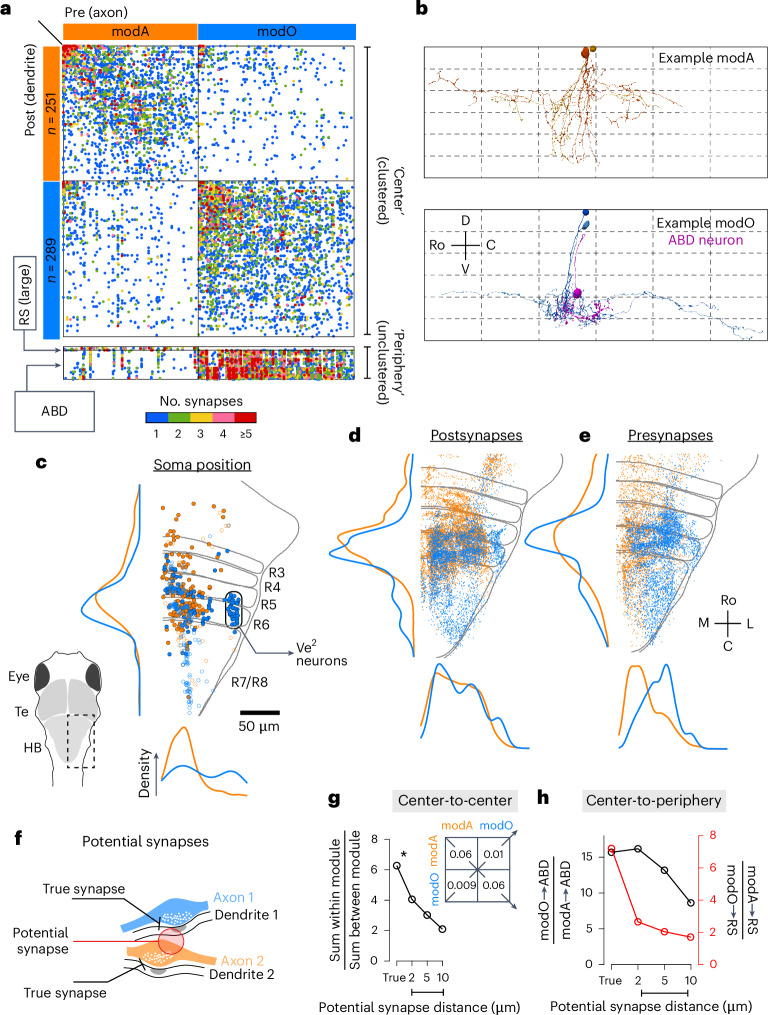
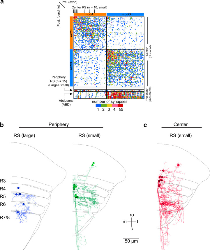
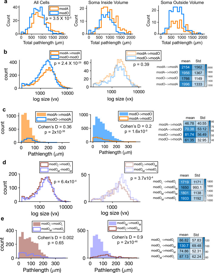
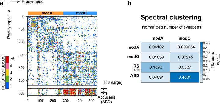
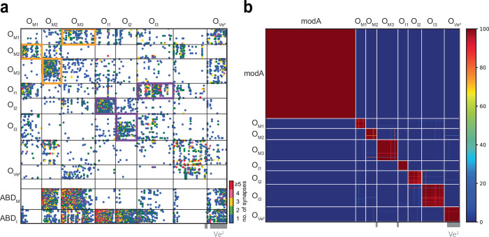
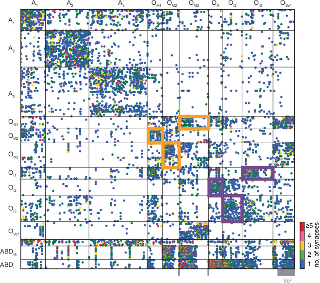
- At the highest level, the recurrent “center” divided into two supermodules: modA (axial/body movement) and modO (oculomotor/eye movement). Based on actual synapses, the wiring specificity index was roughly 6 for center neurons.
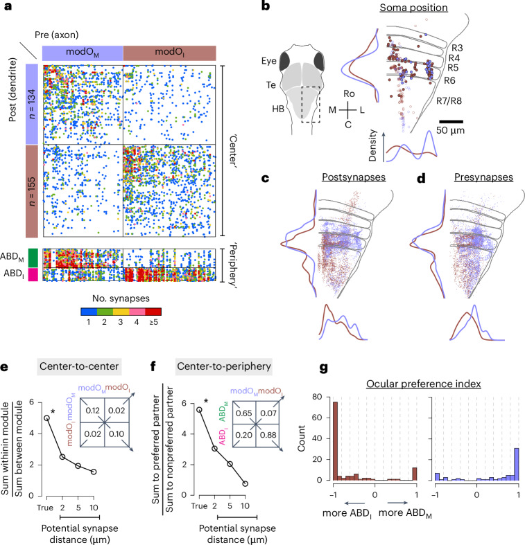
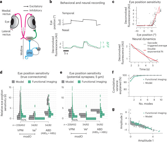
- modO further split into two submodules: modOM and modOI, with neurons in one preferentially connected to ABDM neurons and the other to ABDI neurons; the wiring specificity was almost 6 and the paper reports 5.9 for the hierarchical seven-block organization.
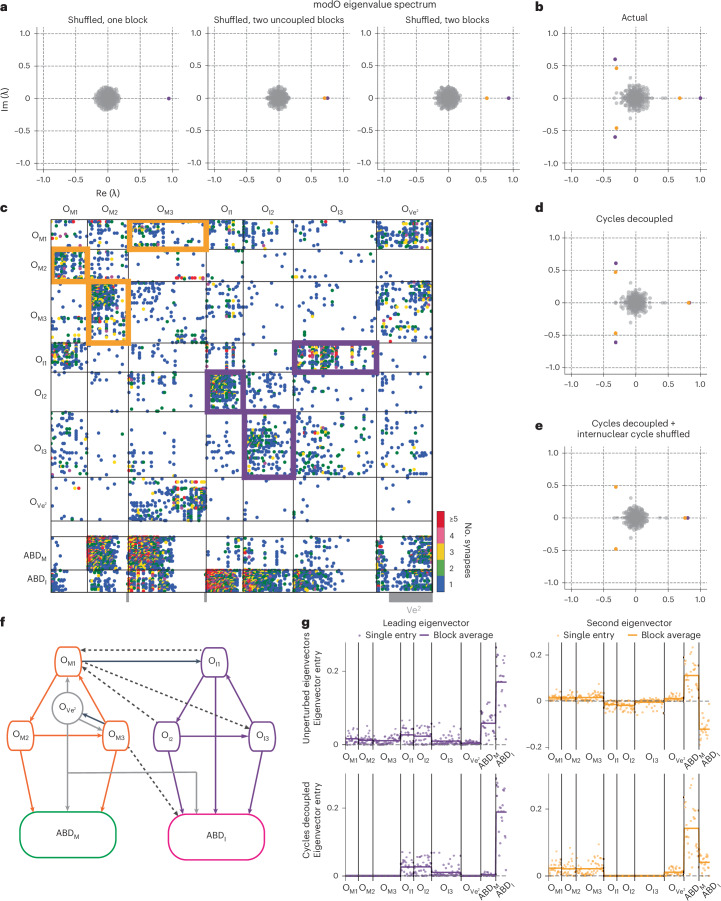
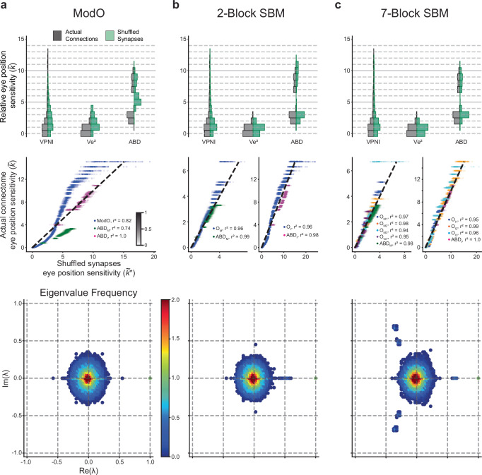
- The modO eigenspectrum indicated two weakly coupled three-block cycles; the paper reports that the motor cycle OM1–OM3 contained 83% of its cells from modOM, while the internuclear cycle OI1–OI3 contained 98% from modOI, and the seventh block was mostly Ve2 neurons (32/34).
Methods
- The authors extended and re-aligned a larval zebrafish brainstem serial-section EM dataset, then used convolutional networks for boundary and synapse detection, followed by human proofreading in Eyewire and skeletonization; the final reconstruction was based on a single animal and included the R4 to R7/R8 region.
- They used graph methods to divide neurons into center vs periphery by eigencentrality, then applied Louvain, spectral clustering, and degree-corrected stochastic block models to identify modules and submodules.
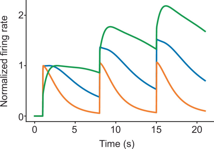
- They built a linear network model directly from the EM-derived synapse counts, normalized by total inputs, and compared simulated eye-position sensitivities and decay dynamics to two-photon calcium imaging data from 20 animals; statistical comparisons included ANOVA on saccade-triggered averages and population-level distribution matching.
Limitations
- The paper explicitly notes that the EM data were acquired from one reimaged animal, and the authors state that they did not predetermine sample size.
- The network model used a minimal set of physiological constraints and a simplified linear rate model; the paper says that single-cell matching might require more sophisticated cell- and synapse-specific biophysics.
- The text makes evident that the imaging and EM datasets came from different fish for the main population-level comparison, so the authors could not do one-to-one cell matching between structure and function.
Model-written summary. Check it against the paper before relying on it.
Integrity signals
Registry
Cites
Statistics
Figures

Verification
Claims the paper makes
14 Valid · 2 Not valid · 15 Not checked · 119 Own results and interpretations
Every source the paper cites for this claim was checked and supports it.
In the paper
“The imaged volume includes neurons involved in eye movements16,21,22,28.”
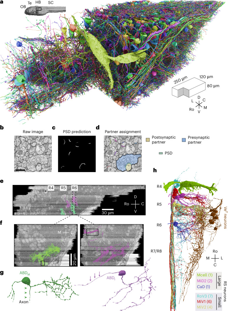
§ Predicting modular functions and neural coding of behavior from a synaptic wiring diagram > Results > Neuronal wiring diagram reconstructed from a vertebrate brainstem We applied serial section EM to reconstruct synaptic connections between neurons in a larval zebrafish brainstem (Fig. 1). The imaged volume includes neurons involved in eye movements16,21,22,28. First, the dataset of Vishwanathan et al.22 was extended by additional imaging of the same serial sections. By improving the alignment of EM images relative to our original work, we created a 3D image stack that was amenable to semiautomated reconstruction29 of 100× more neurons than before. We trained a convolutional neural network to detect neuronal boundaries (Methods)29 and automatically segment the volume. To correct errors in segmentation, we repurposed Eyewire, which was originally developed for proofreading mouse retinal neurons14. Eyewirers proofread ~3,000 objects, which included neurons with cell bodies in the volume as well as ‘orphan’ neurites with no cell body in the volume (Fig. 1a). We will refer to all such objects as ‘neurons’ of the reconstructed network. Convolutional networks were used to automatically detect synaptic clefts and assign presynaptic and postsynaptic partner neurons to each cleft30 (Fig. 1b–d and Methods). The reconstructed dataset contained 2,884 neurons, 44,949 connections between pairs of neurons and 75,163 synapses (additional relevant features are summarized in Supplementary Fig. 1). Most connections (65%) involved just one synapse, but some involved two (19%), three (7.9%), four (3.7%) or more (4.0%) synapses, up to a maximum of 21 (Supplementary Fig. 1a). After registration of our EM volume to the Z-Brain reference atlas31 (Supplementary Fig. 2), several important groups of neurons and neurites were identified (Methods). Comparison with transgenic lines and cranial nerves in the atlas identified the abducens (ABD) neurons that control extraocular muscles, secondary vestibular (Ve2) neurons32 involved in sensorimotor transformations such as the vestibulo-ocular reflex (Fig. 1e–h, Supplementary Fig. 3 and Methods), and two populations of reticulospinal (RS) projection neurons involved in escape behaviors and controlling body movements33–35. The neurons of one RS population were large and dorsally located, and the neurons of the other RS population were smaller and ventromedially located (Fig. 1h and Supplementary Fig. 4).
What the sources say
- Supportedcites [16] Daie, K., Goldman, M. S. & Aksay, E. R. F. Spatial patterns of persistent neural activity vary with the behavioral context of short-term memory. Neuron 85, 847–860 (2015). source
The Results section (“Persistent activity after saccadic and optokinetic stimulation”; page not supplied) says the authors imaged neurons in the horizontal oculomotor integrator of larval zebrafish and recorded their activity during saccadic and optokinetic eye movements. This supports the claim that the imaged volume includes neurons involved in eye movements. (LLM, conf=0.92)
- Supportedcites [21] Lee, M. M., Arrenberg, A. B. & Aksay, E. R. F. A structural and genotypic scaffold underlying temporal integration. J. Neurosci. 35, 7903–7920 (2015). source
The paper's methods and results state that two-photon calcium imaging covered a dorsoventral window in rhombomeres 7-8 of the zebrafish hindbrain ("Two-photon calcium imaging," Methods; "Spatial distribution of the VPNI on a hindbrain genotypic scaffold"), and that neurons within this imaged volume were identified as eye movement-related via correlation of fluorescence with eye position/velocity ("Analysis of cell fluorescence activity"; same Results section, where VPNI cell fluorescence rose with ipsilateral saccades and tracked eye position during OKR). The Abstract likewise frames this cell group (VPNI) as mediating eye-velocity-to-eye-position integration. Thus our copy supports that the imaged volume contains neurons involved in eye movements. (LLM, conf=0.90)
- Supportedcites [22] Vishwanathan, A. et al. Electron microscopic reconstruction of functionally identified cells in a neural integrator. Curr. Biol. 27, 2137–2147 (2017). source
The Introduction says the study imaged and reconstructed neurons in the larval zebrafish oculomotor neural integrator, a circuit involved in controlling eye position. The Abstract identifies the reconstructed neurons by activity correlated with eye position during spontaneous eye movements. (LLM, conf=0.91)
- Supportedcites [28] Schoonheim, P. J., Arrenberg, A. B., Del Bene, F. & Baier, H. Optogenetic localization and genetic perturbation of saccade-generating neurons in zebrafish. J. Neurosci. 30, 7111–7120 (2010). source
The paper's Results section 'Optical stimulation of a small hindbrain area is sufficient for saccade generation' states that the illuminated (and Kaede-photoconverted, hence imaged) volume in the larval zebrafish hindbrain — a narrow column of <100 cells ~20 μm lateral from the midline — contains the neurons necessary and sufficient to elicit a saccade. The section 'A small hindbrain region in rhombomere 5 is necessary for saccade generation' adds that NpHR silencing of that same volume blocked OKR saccades while other regions (pretectum, tectum) had no effect, and the Discussion frames this as localization of eye-movement-generating circuitry. So the volume the paper images/stimulates does include neurons involved in eye movements. (LLM, conf=0.85)
plainSingle case- Asserted: passes — The authors put it forward as true.
- Checkable: passes — It can be checked against evidence.
- Load-bearing: unclear — It is unclear whether the paper’s conclusions depend on it.
- Based: passes — The paper gives a reason why it holds.
- Supported
The cited sources that could be checked couldn’t confirm or dispute this claim.
In the paper
“normalizing by the total number of incoming synapses provides a form of homeostatic synaptic scaling46.”
§ Predicting modular functions and neural coding of behavior from a synaptic wiring diagram > Results > Predicting neural coding and dynamics from the wiring diagram
What the sources say
- Could not verifycites [46] Turrigiano, G. Homeostatic synaptic plasticity: local and global mechanisms for stabilizing neuronal function. Cold Spring Harb. Perspect. Biol. 4, a005736 (2012). sourceExperimental — accuracy not yet measured
The ‘Cell-autonomous, global synaptic scaling of excitatory synapses’ section describes compensatory changes in synaptic strength in response to activity, but does not say that dividing by the total number of incoming synapses produces such scaling. Searches for that normalization rule and for synapse-count normalization found no passage addressing it; the indexed passages provide no page numbers. (LLM, conf=0.76)
plainstates a cause- Asserted: passes — The authors put it forward as true.
- Checkable: passes — It can be checked against evidence.
- Load-bearing: passes — The paper’s conclusions depend on it.
- Based: passes — The paper gives a reason why it holds.
- Could not verify
The cited sources support only part of this claim — read each source’s verdict below.
In the paper
“Together, these subnetworks could provide for maintenance of conjugate and disconjugate eye movements56–58.”
§ Predicting modular functions and neural coding of behavior from a synaptic wiring diagram > Discussion
What the sources say
- Supportedcites [56] Debowy, O. & Baker, R. Encoding of eye position in the goldfish horizontal oculomotor neural integrator. J. Neurophysiol. 105, 896–909 (2011). source
The source's INTRODUCTION (p. 1) lays out exactly this architecture: if eye position is separately encoded for the ipsilateral temporal and contralateral nasal hemifield, 'two subpopulations of neurons are co-localized in each integrator,' bilaterally at least four relatively independent sets of HPNI neurons, with inhibitory/commissural connections 'envisioned to coordinate the nasal and temporal eye position integrator subpopulations for each eye.' The DISCUSSION sections ('Monocular versus conjugate HPNI' and the midline-lesion discussion) report results 'consistent with the presence of monocular and conjugate pathways' and with separate encoding of each eye's time constant (i.e., maintenance of eye position), while the Abstract assigns the ipsilateral vs. conjugate/contralateral populations to abducens motoneurons vs. internuclear neurons and proposes the commissural pathway selects the conjugate/contralateral neurons. The citing sentence is hedged ('could provide'), matching the source's own propositional framing, and covers both conjugate and disconjugate (monocular) maintenance. (LLM, conf=0.82)
- Supportedcites [57] Brysch, C., Leyden, C. & Arrenberg, A. B. Functional architecture underlying binocular coordination of eye position and velocity in the larval zebrafish hindbrain. BMC Biol. 17, 110 (2019). source
The Background describes the oculomotor integrator as maintaining eye position. The Discussion identifies distinct monocular and binocular neuron types, with recruitment differing between monocular and binocular eye movements. Together, these passages support the hedged proposal that the subnetworks could help maintain conjugate and disconjugate movements. (LLM, conf=0.86)
- Partly supportedcites [58] Feierstein, C. E. et al. Dimensionality reduction reveals separate translation and rotation populations in the zebrafish hindbrain. Curr. Biol. 33, 3911–3925 (2023). sourceExperimental — accuracy not yet measured
The Discussion (page unavailable) identifies separate activity modes related to conjugate and vergent eye movements, supporting the proposed distinction between subnetworks. But the Results (page unavailable) describe the vergence cluster mainly in terms of eye velocity, while eye-position representations in the rotation clusters are conjugate. The paper does not establish that these populations maintain both conjugate and disconjugate eye movements. (LLM, conf=0.84)
hedgedstates a possible cause- Asserted: passes — The authors put it forward as true.
- Checkable: passes — It can be checked against evidence.
- Load-bearing: passes — The paper’s conclusions depend on it.
- Based: passes — The paper gives a reason why it holds.
- Supported
Every source the paper cites for this claim was checked and supports it.
In the paper
“the best fits were obtained with an intrinsic time constant of ~1 s”
§ Predicting modular functions and neural coding of behavior from a synaptic wiring diagram > Results > Predicting neural coding and dynamics from the wiring diagram
What the sources say
- Supportedcites [43] Fisher, D., Olasagasti, I., Tank, D. W., Aksay, E. R. F. & Goldman, M. S. A modeling framework for deriving the structural and functional architecture of a short-term memory microcircuit. Neuron 79, 987–1000 (2013). source
The Results section on drift after inactivation says reproducing the observed drift rates required a recurrent excitatory synaptic time constant of approximately 1 second. The Discussion describes the fitted process as intrinsic cellular or synaptic; the claim should not be read as specifying the membrane time constant. Page numbers are unavailable in our copy. (LLM, conf=0.88)
plain- Asserted: passes — The authors put it forward as true.
- Checkable: passes — It can be checked against evidence.
- Load-bearing: passes — The paper’s conclusions depend on it.
- Based: passes — The paper gives a reason why it holds.
- Supported
The sources with a verdict support this claim; the rest weren’t checked yet, have no full text we could read, or their verdicts aren’t rated yet.
In the paper
“Our work similarly informs line attractor network models, for which the VPNI has served as a model system53,54.”
§ Predicting modular functions and neural coding of behavior from a synaptic wiring diagram > Discussion
What the sources say
- Not checked — no full text of the sourcecites [53] Major, G. & Tank, D. Persistent neural activity: prevalence and mechanisms. Curr. Opin. Neurobiol. 14, 675–684 (2004). source
- Supportedcites [54] Joshua, M. & Lisberger, S. G. A tale of two species: neural integration in zebrafish and monkeys. Neuroscience 296, 80–91 (2015). source
In “The architecture of the neural integrator” (page unavailable), the paper describes the oculomotor integrator as a system studied through computational models and says it can operate as a line attractor. “Bridging from zebrafish to monkeys” (page unavailable) models an integrator containing vestibular and prepositus neurons, supporting the identification of the VPNI as a model system. (LLM, conf=0.88)
plainstates an association- Asserted: passes — The authors put it forward as true.
- Checkable: passes — It can be checked against evidence.
- Load-bearing: unclear — It is unclear whether the paper’s conclusions depend on it.
- Based: passes — The paper gives a reason why it holds.
62 more claims
Create a free account to see all 150 claims and to verify the 12 references still open.
- It may state two separate claims as one. 53
- Probably not a substantial claim. 37
- The quote only partly states this claim. 1
Self-check
Percentages, sums and reported differences re-computed from the paper’s own numbers.
Each contradiction between two passages listed here was confirmed by an independent check.
Rated minor: it would not touch a result — a value no result rests on, a p-value that stays on the same side of the significance level, or a conflict that is clerical, resolved elsewhere in the paper, or outside its own findings.
In the paper
§ Predicting modular functions and neural coding of behavior from a synaptic wiring diagram > Methods > Convolutional net training
“We implemented the training and inference of our boundary detectors with the Caffe deep learning framework71.”
§ Predicting modular functions and neural coding of behavior from a synaptic wiring diagram > Methods > Convolutional net training
“The patches were fed into the convolutional network model to perform inference in PyTorch75.”
Citations
Cites
U-Net: Convolutional Networks for Biomedical Image Segmentation
Ronneberger, O., Fischer, P., & Brox, T. (2015) · Lecture notes in computer science · doi:10.1007/978-3-319-24574-4_28 · Cited by 99,404 · cited 2×
“The final model used an RS-U-Net architecture 73 implemented using PyTorch 75 and was trained using a manual learning rate schedule, decreasing the rate by a factor of 10 when the smoothed validation error converged.”
Adam: A Method for Stochastic Optimization
Kingma, D. P., & Ba, J. (2014) · arXiv · doi:10.48550/arxiv.1412.6980 · Cited by 98,946
Batch Normalization: Accelerating Deep Network Training by Reducing Internal Covariate Shift
Ioffe, S., & Szegedy, C. (2015) · arXiv · doi:10.48550/arxiv.1502.03167 · Cited by 27,818
Fast unfolding of communities in large networks
Blondel, V. D., Guillaume, J.-L., Lambiotte, R., & Lefebvre, E. (2008) · Journal of Statistical Mechanics: Theory and Experiment · doi:10.1088/1742-5468/2008/10/p10008 · Cited by 21,424 · cited 1×
“Graph clustering was performed using the Louvain clustering algorithm 83 for identifying different ‘communities’ or ‘modules’ in an interconnected network by optimizing the ‘modularity’ of the network, where modularity measures the (weighted) density of connections within a module compared to…”
(2017) · Cited by 11,625
Complex network measures of brain connectivity: Uses and interpretations
Rubinov, M., & Sporns, O. (2010) · NeuroImage · doi:10.1016/j.neuroimage.2009.10.003 · Cited by 11,522
Caffe: Convolutional Architecture for Fast Feature Embedding
Jia, Y., Shelhamer, E., Donahue, J., Karayev, S., Long, J., Girshick, R., Guadarrama, S., & Darrell, T. (2014) · Proceedings of the 22nd ACM international conference on Multimedia · doi:10.1145/2647868.2654889 · Cited by 11,077 · cited 1×
“We implemented the training and inference of our boundary detectors with the Caffe deep learning framework 71 .”
Caffe: Convolutional Architecture for Fast Feature Embedding
Jia, Y., Shelhamer, E., Donahue, J., Karayev, S., Long, J., Girshick, R., Guadarrama, S., & Darrell, T. J. (2014) · arXiv (Cornell University) · doi:10.48550/arxiv.1408.5093 · Cited by 3,752 · cited 1×
“We implemented the training and inference of our boundary detectors with the Caffe deep learning framework 71 .”
Design Rules: The Power of Modularity
Baldwin, C. Y., & Clark, K. B. (2000) · doi:10.7551/mitpress/2366.001.0001 · Cited by 3,504
Stochastic blockmodels: First steps
Holland, P. W., Laskey, K. B., & Leinhardt, S. (1983) · Social Networks · doi:10.1016/0378-8733(83)90021-7 · Cited by 2,755 · cited 8×
“We separately applied an SBM to modA and examined how axial sub-modules aligned with those from modO.”
Influential
Research works printed but not linked: 4
- Anderson, J. R. et al. Exploring the retinal connectome. Mol. Vis. 17, 355–379 (2011).
- Allen, W. F. Formatio reticularis and reticulospinal tracts, their visceral functions and possible relationships to tonicity and clonic contractions. J. Wash. Acad. Sci. 22, 490–495 (1932).
- Skaggs, W. E., Knierim, J. J., Kudrimoti, H. S. & McNaughton, B. L. A model of the neural basis of the rat’s sense of direction. Adv. Neural Inf. Process. Syst. 7, 173–180 (1995).
- Newman, M. Networks (Oxford University Press, 2018).
Cited by
A brainstem integrator for self-location memory and positional homeostasis in zebrafish
Yang, E., Zwart, M., James, B., Rubinov, M., Wei, Z., Narayan, S., Vladimirov, N., Mensh, B. D., Fitzgerald, J. E., & Ahrens, M. B. (2022) · Cell · doi:10.1016/j.cell.2022.11.022 · Cited by 71
Dowell, C. K., Hawkins, T. A., & Bianco, I. H. (2025) · Current Biology · doi:10.1016/j.cub.2024.12.010 · Cited by 18
“This independence of the two neuronal types in nVI is supported by a recent connectomics study, which identified two oculomotor submodules in the zebrafish tegmentum, which are preferentially connected to either INNs or LRMNs. 65 70 In zebrafish, a likely candidate for these EBNs are the neurons we reconstructed in dorsa…”
Prediction of neural activity in connectome-constrained recurrent networks
Beirán, M., & Litwin-Kumar, A. (2025) · Nature Neuroscience · doi:10.1038/s41593-025-02080-4 · Cited by 39
“5), we modeled systems for which detailed descriptions of the function of individual cell types exist 16,41,42 .”
InfluentialPrediction of neural activity in connectome-constrained recurrent networks
Beiran, M., & Litwin-Kumar, A. (2024) · doi:10.1101/2024.02.22.581667 · Cited by 16
Infrequent strong connections constrain connectomic predictions of neuronal function
Currier, T. A., & Clandinin, T. R. (2025) · Cell · doi:10.1016/j.cell.2025.05.007 · Cited by 20
Metadata
- Authors
- Vishwanathan, A., Sood, A., Wu, J., Ramirez, A. D., Yang, R., Kemnitz, N., Ih, D., Turner, N., Lee, K., Tartavull, I., Silversmith, W. M., Jordan, C. S., David, C., Bland, D., Sterling, A., Seung, H. S., Goldman, M. S., Aksay, E. R. F., Eyewirers, T., Wille, K., Silverman, B., Willie, R., Morejohn, S., Koolman, S., Sorek, M., Jones, D., Sterling, A., David, C., Reddy, S., Pelegrino, A., & Williams, S.
- Affiliations
- Princeton University (US)
- University of California, Davis (US)
- SUNY Downstate Health Sciences University (US)
- Weill Cornell Medicine (US)
- Corresponding author
- Vishwanathan, Ashwin
- Goldman, Mark S.
- Aksay, Emre R. F.
- ORCID
- Venue
- Nature Neuroscience
- Published
- 2024-11-22
- Volume
- 27
- Issue
- 12
- Pages
- 2443-2454
- ISSN
- 1097-6256 (ISSN-L)
- 1546-1726
- PMC
- PMC11614741
- OpenAlex
- W4404612853
- Cited by
- 36
- References
- 100
- Citations by year
- 2026: 5 · 2025: 17 · 2024: 1
- FWCI
- 4.32
- Type
- journal article
- Language
- en
- Open access
- hybrid
- doi.org
- Licence
- cc-by-nc-nd
- creativecommons.org/licenses/by-nc-nd/4.0 (tdm)
- creativecommons.org/licenses/by-nc-nd/4.0 (vor)
- Locations
- Nature Neuroscience (publishedVersion, cc-by-nc-nd)
- bioRxiv (Cold Spring Harbor Laboratory) (submittedVersion, cc-by-nd)
- PubMed Central (publishedVersion, cc-by-nc-nd)
- PubMed (publishedVersion)
- eScholarship (California Digital Library) (submittedVersion, cc-by-nc-nd)
- Funders
- U.S. Department of Health & Human Services | NIH | National Eye Institute (EY021581, EY027036, EY027017)
- U.S. Department of Health & Human Services | NIH | National Institute of Neurological Disorders and Stroke (NS104682)
- U.S. Department of Health & Human Services | NIH | NCI | Division of Cancer Epidemiology and Genetics, National Cancer Institute (CA203710)
- Topics
- Life Sciences › Neuroscience › Cognitive Neuroscience › Neural dynamics and brain function
- Life Sciences › Neuroscience › Cellular and Molecular Neuroscience › Neuroscience and Neuropharmacology Research
- Social Sciences › Education › Undergraduate Neuroscience Education and Research
- Keywords
- connectome, oculomotor control, eye movements, body movement, positive feedback, attractor dynamics, neural coding, eye position, neural network model, calcium imaging
- MeSH terms
- Animals, Behavior, Animal, Brain Stem, Eye Movements, Larva, Models, Neurological, Nerve Net, Neural Pathways, Neurons, Synapses, Zebrafish, Neural Networks, Computer, Connectome
About these checks
Registry, retraction, Cites and statistics results are computed, not judged, with one exception: a printed reference that no index lists is read once by a model before it counts as a citation error. Claims are extracted by a model and kept only when their quote appears verbatim in the text; each cited source is then checked, with a model’s help, for whether it says what the claim relies on. Those verdicts can be wrong — read the claim’s quote and the cited source before relying on one.
The claim verdicts this report counts are experimental: their accuracy is not yet measured.
A language model drew the claims from the paper on 2026-10-10, under version 3 of the claim definition (model deepseek-v4.1-flash, prompt extract-v3).
A second model labelled each claim on 2026-10-10 (model jev-1.13-20260917, definition revision gold-guideline-v0.2).
Cited sources are checked with a language model’s help (gpt-6-sol and qwen3.8-omni-flash).
Statistics and arithmetic are recomputed, not judged.
Confidence bands are shown only for fields calibrated on our annotated test set. None is calibrated yet, so no band is shown.
What counts as a claim ›How we measure confidence ›How we check this ›
Are you an author, or do you see a problem with this page? Request a review
How to cite
Cite CoChat for the checks on this page, and the paper for its own findings.
- This page
- CoChat. (2026). Citation check: Predicting modular functions and neural coding of behavior from a synaptic wiring diagram. https://app.cochat.ai/papers/10.1038/s41593-024-01784-3
- The paper
- Vishwanathan, A., Sood, A., Wu, J., Ramirez, A. D., Yang, R., Kemnitz, N., Ih, D., Turner, N., Lee, K., Tartavull, I., Silversmith, W. M., Jordan, C. S., David, C., Bland, D., Sterling, A., Seung, H. S., Goldman, M. S., Aksay, E. R. F., Eyewirers, T., . . . Williams, S. (2024). Predicting modular functions and neural coding of behavior from a synaptic wiring diagram. Nature Neuroscience. https://doi.org/10.1038/s41593-024-01784-3
Data sources
Bibliographic data: Semantic Scholar, OpenAlex, Crossref.
Contains information from the Semantic Scholar Academic Graph Datasets, made available under the ODC Attribution License (ODC-BY 1.0).
Semantic Scholar’s data is described in: Kinney, R., et al. (2023). The Semantic Scholar Open Data Platform. arXiv:2301.10140.
