

Hierarchical Models in the Brain
Open accessThe DOI matches its Crossref record; 94 of the 102 references it cites were found in a registry or an index; 10 of the 81 sources its claims cite were checked for support.
Abstract
This paper describes a general model that subsumes many parametric models for continuous data. The model comprises hidden layers of state-space or dynamic causal models, arranged so that the output of one provides input to another. The ensuing hierarchy furnishes a model for many types of data, of arbitrary complexity. Special cases range from the general linear model for static data to generalised convolution models, with system noise, for nonlinear time-series analysis. Crucially, all of these models can be inverted using exactly the same scheme, namely, dynamic expectation maximization. This means that a single model and optimisation scheme can be used to invert a wide range of models. We present the model and a brief review of its inversion to disclose the relationships among, apparently, diverse generative models of empirical data. We then show that this inversion can be formulated as a simple neural network and may provide a useful metaphor for inference and learning in the brain.
Overview
CoChat Summary
## TL;DR
This paper presents hierarchical dynamic models (HDMs) as a very general framework that contains many familiar static and dynamic statistical models as special cases, all invertible with the same dynamic expectation maximization (DEM) scheme. It argues that the same inversion can be written as a simple neural network and may serve as a metaphor for inference and learning in the brain.
## Key findings
- HDMs “subsum[e] many parametric models for continuous data,” ranging from the general linear model for static data to generalized convolution models with system noise for nonlinear time-series analysis.
- The paper claims that these diverse models can all be inverted using the same scheme, dynamic expectation maximization (DEM), under a Laplace/mean-field variational approximation.
- In the results, the author shows that HDMs encompass standard tools including the general linear model, expectation maximization (EM), restricted maximum likelihood (ReML), covariance component estimation, Gaussian process models, PCA, factor analysis, ICA, sparse coding, deconvolution, and state-space filtering.
- A worked example is described in which DEM converged in “about sixteen iterations” using embedding order “n = 6” and roughness hyperparameter “γ = 4,” with the text stating that the recovered states, parameters, and hyperparameters closely matched the true values and that the true values lay largely within the 90% confidence intervals.
## Methods
- The paper develops a hierarchical dynamic model in generalized coordinates of motion, with hidden states and causes organized across levels; the model includes Gaussian priors and Gaussian assumptions about fluctuations, and uses prediction errors at each level.
- Inversion is based on variational Bayes under mean-field and Laplace approximations, optimizing free energy / variational action with a dynamic expectation maximization scheme that separates D-step (states), E-step (parameters), and M-step (hyperparameters).
- The paper then maps this inversion scheme onto a neural-network-like message-passing architecture and illustrates the framework with analytic special cases and a simulation example.
## Limitations
- The paper states that the Laplace/Gaussian approximation “restrict[s] recognition to unimodal probabilistic representations,” though it frames this as a practical simplification.
- The text makes evident that many claims are theoretical and illustrative rather than empirically validated in this paper; it says the neuronal implementation “calls for an enormous amount of empirical verification and hypothesis testing” (evident in the text).
- The paper also makes evident that the examples and special-case derivations cover only a “partial list” of possible models, so the treatment is not exhaustive (evident in the text).
Model-written summary. Check it against the paper before relying on it.
Integrity signals
Registry
Cites
Statistics
Figures



Verification
Claims the paper makes
9 Valid · 2 Not valid · 48 Not checked · 185 Own results and interpretations
The cited sources support only part of this claim — read each source’s verdict below.
In the paper
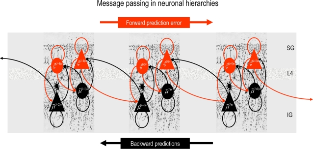
“There is a key functional asymmetry between forward and backward connections that renders backward connections more modulatory or nonlinear in their effects on neuronal responses (e.g., [44]; see also Hupe et al. [47]).”
§ Hierarchical Models in the Brain > Results > Neuronal Implementation
What the sources say
- Partly supportedcites [44] SM Sherman, 1998, On the actions that one nerve cell can have on another: distinguishing “drivers” from “modulators”., Proc Natl Acad Sci U S A sourceExperimental — accuracy not yet measured
In the paper’s discussion of lateral geniculate inputs (indexed as Abstract; page unavailable), retinal inputs are treated as drivers, while inputs from cortex are described as modulators. That supports a forward-versus-backward distinction for this thalamic relay, but the Conclusions say that classifying corticocortical pathways remains largely untested; the paper does not establish the claimed general asymmetry or characterize backward effects as nonlinear. (LLM, conf=0.84)
- Not checked — no full text of the sourcecites Hupe et al. [47] JM Hupe, 1998, Cortical feedback improves discrimination between figure and background by V1, V2 and V3 neurons., Nature source
plainstates a cause- Asserted: passes — The authors put it forward as true.
- Checkable: passes — It can be checked against evidence.
- Load-bearing: passes — The paper’s conclusions depend on it.
- Based: passes — The paper gives a reason why it holds.
- Partly supported
The sources with a verdict support this claim; the rest weren’t checked yet, have no full text we could read, or their verdicts aren’t rated yet.
In the paper
“This selective modulation of afferents mirrors the gain-control mechanisms invoked for attention; e.g., [58],[59].”
§ Hierarchical Models in the Brain > Results > Neuronal Implementation
What the sources say
- Not checked — no full text of the sourcecites [58] S Treue, 1996, Attentional modulation of visual motion processing in cortical areas MT and MST., Nature source
- Supportedcites [59] JC Martinez-Trujillo, 2004, Feature-based attention increases the selectivity of population responses in primate visual cortex., Curr Biol source
The Conclusions (page unavailable) state that feature-based attention multiplicatively modulates neuronal responses in line with a feature-similarity gain model. This supports the cited comparison to attentional gain control; the sentence does not attribute the modulation of afferents themselves to this paper. (LLM, conf=0.88)
plainstates an association- Asserted: passes — The authors put it forward as true.
- Checkable: passes — It can be checked against evidence.
- Load-bearing: passes — The paper’s conclusions depend on it.
- Based: passes — The paper gives a reason why it holds.
The cited sources support only part of this claim — read each source’s verdict below.
In the paper
“Functional asymmetries in forwards (linear) and backwards (nonlinear) connections may reflect their distinct roles in recognition (c.f., [44]).”
§ Hierarchical Models in the Brain > Results > Neuronal Implementation
What the sources say
- Partly supportedcites [44] SM Sherman, 1998, On the actions that one nerve cell can have on another: distinguishing “drivers” from “modulators”., Proc Natl Acad Sci U S A sourceExperimental — accuracy not yet measured
The paper distinguishes driver inputs, which transmit receptive-field properties, from modulator inputs, which alter transmission (Abstract; page unavailable). It also discusses different possible roles for thalamocortical and corticothalamic pathways. It does not characterize forward connections as linear or backward connections as nonlinear, or link those properties to recognition; the Conclusions say corticocortical pathway classifications remain largely untested. (LLM, conf=0.76)
hedgedstates a possible cause- Asserted: passes — The authors put it forward as true.
- Checkable: passes — It can be checked against evidence.
- Load-bearing: unclear — It is unclear whether the paper’s conclusions depend on it.
- Based: passes — The paper gives a reason why it holds.
- Partly supported
Every source the paper cites for this claim was checked and supports it.
In the paper
“Arguments like this suggest that free-form approximations and their attending sampling schemes are not really viable in a neuronal context (although they have been considered; see [86] and above)”
§ Hierarchical Models in the Brain > Discussion
What the sources say
- Supportedcites [86] TS Lee, 2003, Hierarchical Bayesian inference in the visual cortex., J Opt Soc Am A source
The citation is attached to the parenthetical point that sampling-based approximations have been considered in a neuronal context, not to the citing authors’ conclusion that they are unviable. In “Particle Filtering and Bayesian Belief Propagation,” Lee and Mumford discuss weighted samples as an approximation to perceptual probability distributions; the Introduction proposes particle filtering as a possible cortical algorithm. The source does not endorse the unviability conclusion. (LLM, conf=0.92)
hedgedstates a cause- Asserted: passes — The authors put it forward as true.
- Checkable: passes — It can be checked against evidence.
- Load-bearing: passes — The paper’s conclusions depend on it.
- Based: passes — The paper gives a reason why it holds.
- Supported
The cited sources that could be checked couldn’t confirm or dispute this claim.
In the paper
“Lateral interactions may encode the relative precision of prediction errors and change in a way that is consistent with classical neuromodulation (c.f., [63],[71]).”
§ Hierarchical Models in the Brain > Results > Neuronal Implementation
What the sources say
- Not checked — no full text of the sourcecites [63] AJ Yu, 2005, Uncertainty, neuromodulation and attention., Neuron source
- Could not verifycites [71] Y Niv, 2005, Dopamine, uncertainty and TD learning., Behav Brain Funct sourceExperimental — accuracy not yet measured
The Discussion (page unavailable) addresses asymmetric dopamine coding of prediction errors and mentions a possible opponent neurotransmitter. Searches for lateral interactions, relative precision, and neuromodulation found no passage saying that lateral interactions encode precision or change in the claimed way. (LLM, conf=0.76)
hedgedstates a possible cause- Asserted: passes — The authors put it forward as true.
- Checkable: passes — It can be checked against evidence.
- Load-bearing: passes — The paper’s conclusions depend on it.
- Based: passes — The paper gives a reason why it holds.
122 more claims · 1 with their cited sources checked
Create a free account to see all 244 claims and to verify the 3 references still open.
- Probably not a substantial claim. 65
- It may state two separate claims as one. 65
- The quote only partly states this claim. 1
Claims other papers make about this one
Each is checked against this paper’s own text: does it say what the citing paper says it does?
The source backs part of the claim, not all of it — or backs it for a different population, condition or comparison.
In the citing paper
“This equation says that the contribution of any (angular) frequency ω in the prediction errors (encoded by superficial pyramidal cells) to the expectations (encoded by the deep pyramidal cells) is suppressed in proportion to that frequency (Friston 2008). In other words, high frequencies should be attenuated when passing from superficial to deep pyramidal cells.”
From Canonical Microcircuits for Predictive Coding (2012) · cites this paper as Friston 2008
Experimental — accuracy not yet measuredThe source backs part of the claim, not all of it — or backs it for a different population, condition or comparison.
In the citing paper
“and lies in the integrity of neuromodulatory function (2).”
From A more precise look at context in autism (2015) · cites this paper as [2]
Experimental — accuracy not yet measuredThe source backs part of the claim, not all of it — or backs it for a different population, condition or comparison.
In the citing paper
“its solutions grandfather nearly every known statistical estimation scheme, under parametric assumptions about additive or multiplicative noise (Friston, 2008)”
From The Computational Anatomy of Psychosis (2013) · cites this paper as Friston, 2008
Experimental — accuracy not yet measuredThe source backs part of the claim, not all of it — or backs it for a different population, condition or comparison.
In the citing paper
“Predictive coding is a process theory with a biologically plausible back story and a considerable amount of empirical support [21,22].”
From Active interoceptive inference and the emotional brain (2016) · cites this paper as [21]
Experimental — accuracy not yet measuredThe source backs part of the claim, not all of it — or backs it for a different population, condition or comparison.
In the citing paper
“Cortical bias or gain control is mediated by intrinsic inhibitory connections within cortical sources, which rescale prediction errors, in proportion to their precision, so that as precision increases intrinsic recurrent inhibition decreases (Abbott et al., 1997, Friston, 2008).”
From The functional anatomy of schizophrenia: A dynamic causal modeling study of predictive coding (2014) · cites this paper as Friston, 2008
Experimental — accuracy not yet measured
18 more claims about this paper
Create a free account to see every claim other papers make about this one.
Citations
Cites
Maximum Likelihood from Incomplete Data Via the EM Algorithm
Dempster, A. P., Laird, N. M., & Rubin, D. B. (1977) · Journal of the Royal Statistical Society Series B: Statistical Methodology · doi:10.1111/j.2517-6161.1977.tb01600.x · Cited by 50,444 · cited 1×
“We have discussed static cases of this fixed-form scheme previously and how it reduces to expectation maximisation ( EM ; [17]) and restricted maximum likelihood ( ReML ; [18]) for linear models [15].”
BackgroundA New Approach to Linear Filtering and Prediction Problems
Kalman, R. E. (1960) · Journal of Basic Engineering · doi:10.1115/1.3662552 · Cited by 31,751 · cited 1×
“The conventional approach to online Bayesian tracking of nonlinear or non-Gaussian systems employs extended Kalman filtering [30] or sequential Monte Carlo methods such as particle filtering.”
MethodLearning Internal Representations by Error Propagation
Rumelhart, D. E., Hinton, G. E., & Williams, R. J. (1985) · doi:10.21236/ada164453 · Cited by 16,172
An Information-Maximization Approach to Blind Separation and Blind Deconvolution
Bell, A. J., & Sejnowski, T. J. (1995) · Neural Computation · doi:10.1162/neco.1995.7.6.1129 · Cited by 8,986 · cited 1×
“) decomposes the observed response into a linear mixture of non-Gaussian causes”
Neural Mechanisms of Selective Visual Attention
Desimone, R., & Duncan, J. (1995) · Annual Review of Neuroscience · doi:10.1146/annurev.ne.18.030195.001205 · Cited by 8,388
Distributed hierarchical processing in the primate cerebral cortex
Felleman, D. J., & Van Essen, D. C. (1991) · Cerebral Cortex · doi:10.1093/cercor/1.1.1 · Cited by 7,783 · cited 2×
“This means we would expect to see connections reciprocated in the brain, which is generally the case [39,40].”
BackgroundStochastic Processes and Filtering Theory
(1970) · Mathematics in Science and Engineering · doi:10.1016/s0076-5392(09)x6022-4 · Cited by 7,302
Emergence of simple-cell receptive field properties by learning a sparse code for natural images
Olshausen, B. A., & Field, D. J. (1996) · Nature · doi:10.1038/381607a0 · Cited by 5,694 · cited 1×
“In the same way that factor analysis is a generalisation of PCA to non-Gaussian causes, ICA can be extended to form sparse-coding models of the sort proposed by Olshausen and Fields [37] by allowing observation error.”
MethodRao, R. P. N., & Ballard, D. H. (1999) · Nature Neuroscience · doi:10.1038/4580 · Cited by 5,483 · cited 2×
“The mean-field approximation q ( W )= q ( u ( t )) q ( h ) q ( l ) enables inference about perceptual states, causal regularities and context, without representing the joint distribution explicitly; c.f., [64].”
BackgroundA theory of cortical responses.
Friston, K. (2005) · Philosophical Transactions of the Royal Society B: Biological Sciences · doi:10.1098/rstb.2005.1622 · Cited by 4,578 · cited 2×
“We have laid out the neurobiological and psycho-physical motivation for the neuronal implementation of DEM in [3] and [4].”
MethodSelf-citationProbabilistic Principal Component Analysis
Tipping, M. E., & Bishop, C. M. (1999) · Journal of the Royal Statistical Society Series B: Statistical Methodology · doi:10.1111/1467-9868.00196 · Cited by 3,679 · cited 1×
“, S = lI, this is also known as a probabilistic PCA model [35].”
BackgroundPreface: Cerebral Cortex Has Come of Age
Goldman-Rakic, P. S., & Rakic, P. (1991) · Cerebral Cortex · doi:10.1093/cercor/1.1.1-a · Cited by 3,393
The Theory of Stochastic Processes
Cox, D. R., Miller, H. D., Weiss, G., & Shuler, K. (1966) · Physics Today · doi:10.1063/1.3047872 · Cited by 3,324
Mesulam, M. (1998) · Brain · doi:10.1093/brain/121.6.1013 · Cited by 3,072 · cited 1×
“A key architectural principle of the brain is its hierarchical organisation [38–41].”
BackgroundSynaptic Plasticity and Memory: An Evaluation of the Hypothesis
Martin, S. J., Grimwood, P. D., & Morris, R. G. M. (2000) · Annual Review of Neuroscience · doi:10.1146/annurev.neuro.23.1.649 · Cited by 2,794 · cited 1×
“These theoretical predictions are entirely consistent with empirical and computational characterisations of plasticity [56,57].”
ResultMaximum Likelihood Approaches to Variance Component Estimation and to Related Problems
Harville, D. A. (1977) · Journal of the American Statistical Association · doi:10.1080/01621459.1977.10480998 · Cited by 2,667 · cited 2×
“It is interesting to note that the ReML objective function and the variational energy are formally identical under this model [15,18].”
BackgroundMethod(1998) · Springer eBooks · doi:10.1007/978-94-011-5014-9 · Cited by 2,418
A View of the Em Algorithm that Justifies Incremental, Sparse, and other Variants
Neal, R. M., & Hinton, G. E. (1998) · Learning in Graphical Models · doi:10.1007/978-94-011-5014-9_12 · Cited by 2,187
CORTICAL PLASTICITY: From Synapses to Maps
Buonomano, D. V., & Merzenich, M. M. (1998) · Annual Review of Neuroscience · doi:10.1146/annurev.neuro.21.1.149 · Cited by 2,083 · cited 1×
“These theoretical predictions are entirely consistent with empirical and computational characterisations of plasticity [56,57].”
ResultTopics in the Theory of Random Noise
Medhurst, R. G. (1969) · Electronics and Power · doi:10.1049/ep.1969.0039 · Cited by 2,049 · cited 7×
“…this is a convenient assumption that is exploited in conventional Bayesian filtering schemes and appropriate for physical systems with Brownian processes, it is less plausible for biological and other systems, where random fluctuations are themselves generated by dynamical systems ([6], p 81).”
BackgroundMethodInfluentialUncertainty, Neuromodulation, and Attention
Yu, A. J., & Dayan, P. (2005) · Neuron · doi:10.1016/j.neuron.2005.04.026 · Cited by 1,774 · cited 3×
“The physiological aspects of these dynamics provide an interesting substrate for attentional mechanisms in the brain (see Schroeder et al., [62] for review) and are not unrelated to the ideas in [63].”
BackgroundResultInfluentialSynaptic depression and cortical gain control
Abbott, L. F., Varela, J. A., Sen, K., & Nelson, S. B. (1997) · Science · doi:10.1126/science.275.5297.221 · Cited by 1,690 · cited 1×
“N The rescaling of prediction errors by recurrent connections, in proportion to their precision, affords a form of cortical bias or gain control [73,74].”
BackgroundBarlow, H. B. (1989) · Neural Computation · doi:10.1162/neco.1989.1.3.295 · Cited by 1,650
Maunsell, J., & van Essen, D. (1983) · The Journal of Neuroscience · doi:10.1523/jneurosci.03-12-02563.1983 · Cited by 1,602 · cited 1×
“A key architectural principle of the brain is its hierarchical organisation [38–41].”
BackgroundPredictive coding under the free-energy principle
Friston, K., & Kiebel, S. (2009) · Philosophical Transactions of the Royal Society B: Biological Sciences · doi:10.1098/rstb.2008.0300 · Cited by 1,579
Self-citationHierarchical Bayesian inference in the visual cortex
Lee, T. S., & Mumford, D. (2003) · Journal of the Optical Society of America A · doi:10.1364/josaa.20.001434 · Cited by 1,473 · cited 1×
“Arguments like this suggest that free-form approximations and their attending sampling schemes are not really viable in a neuronal context (although they have been considered; see [86] and above) The third choice was a mean-field approximation; q(W) = q(u(t))q(h)q(l).”
BackgroundMultiple dopamine functions at different time courses
Schultz, W. (2007) · Annual Review of Neuroscience · doi:10.1146/annurev.neuro.28.061604.135722 · Cited by 1,415 · cited 1×
“In this figure, we have focused on means or expectations m i of the marginal densities, q ( W i )= N ( W i : m i , C i ). doi:10.1371/journal.pcbi.1000211.g010 have been implicated in value-learning [68–70], attention and the encoding of uncertainty [63,71].”
BackgroundInfluentialA free energy principle for the brain
Friston, K., Kilner, J., & Harrison, L. (2006) · Journal of Physiology-Paris · doi:10.1016/j.jphysparis.2006.10.001 · Cited by 1,369 · cited 3×
“These observations pertain to the anatomy and physiology of neuronal architectures; see Friston et al. [5] for a discussion of operational and cognitive issues, under a free-energy principle for the brain.”
BackgroundInfluentialSelf-citationChen, T., & Chen, H. (1995) · IEEE Transactions on Neural Networks · doi:10.1109/72.392253 · Cited by 1,230 · cited 1×
“However, unlike back propagation of errors or universal approximation in neural networks [22], DEM is not simply a nonlinear function approximation device.”
BackgroundDayan, P., Hinton, G. E., Neal, R. M., & Zemel, R. S. (1995) · Neural Computation · doi:10.1162/neco.1995.7.5.889 · Cited by 1,207 · cited 1×
“, [90,91]).”
The Theory of Stochastic Processes.
Bartholomew, D. J., Cox, D. R., & Miller, H. D. (1966) · Journal of the Royal Statistical Society. Series A (General) · doi:10.2307/2343509 · Cited by 1,193
London, M., & Häusser, M. (2005) · Annual Review of Neuroscience · doi:10.1146/annurev.neuro.28.061604.135703 · Cited by 1,149 · cited 1×
“This induces a hierarchy over levels and, within each level, a hierarchical relationship between states, where hidden states predict causes. doi:10.1371/journal.pcbi.1000211.g008 activation function that models nonlinear summation of presynaptic inputs over the dendritic tree [55].”
BackgroundInfluentialA neural basis for visual search in inferior temporal cortex
Chelazzi, L., Miller, E. K., Duncan, J., & Desimone, R. (1993) · Nature · doi:10.1038/363345a0 · Cited by 1,114 · cited 1×
“Furthermore, they enact the sorts of mechanisms implicated in biased competition models of spatial and object-based attention mediating visual search [60,61].”
BackgroundOn the computational architecture of the neocortex: II The role of cortico-cortical loops
Mumford, D. (1992) · Biological Cybernetics · doi:10.1007/bf00198477 · Cited by 1,074
The functional logic of cortical connections
Zeki, S., & Shipp, S. (1988) · Nature · doi:10.1038/335311a0 · Cited by 1,067 · cited 3×
“This means we would expect to see connections reciprocated in the brain, which is generally the case [39,40].”
BackgroundMethodLaminar origins and terminations of cortical connections of the occipital lobe in the rhesus monkey
Rockland, K. S., & Pandya, D. N. (1979) · Brain Research · doi:10.1016/0006-8993(79)90485-2 · Cited by 1,060 · cited 1×
“The neurobiological notion of a hierarchy rests upon the distinction between forward and backward connections [42–45].”
BackgroundNeural mechanisms for visual memory and their role in attention
Desimone, R. (1996) · Proceedings of the National Academy of Sciences · doi:10.1073/pnas.93.24.13494 · Cited by 1,028 · cited 1×
“Furthermore, they enact the sorts of mechanisms implicated in biased competition models of spatial and object-based attention mediating visual search [60,61].”
BackgroundAttentional modulation of visual motion processing in cortical areas MT and MST
Treue, S., & Maunsell, J. H. R. (1996) · Nature · doi:10.1038/382539a0 · Cited by 1,025
Keeping the neural networks simple by minimizing the description length of the weights
Hinton, G. E., & van Camp, D. (1993) · Proceedings of the sixth annual conference on Computational learning theory - COLT '93 · doi:10.1145/168304.168306 · Cited by 994
Stein's Estimation Rule and its Competitors—An Empirical Bayes Approach
Efron, B., & Morris, C. (1973) · Journal of the American Statistical Association · doi:10.1080/01621459.1973.10481350 · Cited by 981 · cited 1×
“In empirical Bayes [9], factorisations of the likelihood create empirical priors that share properties of both the likelihood and priors.”
BackgroundJONES, J. E. (1971) · Nature · doi:10.1038/233571b0 · Cited by 952
On the computational architecture of the neocortex: I. The role of the thalamo-cortical loop
Mumford, D. (1991) · Biological Cybernetics · doi:10.1007/bf00202389 · Cited by 929
Topics in the Theory of Random Noise
(1970) · USSR Computational Mathematics and Mathematical Physics · doi:10.1016/0041-5553(70)90203-x · Cited by 895
Variational free energy and the Laplace approximation
Friston, K., Mattout, J., Trujillo-Barreto, N., Ashburner, J., & Penny, W. (2007) · NeuroImage · doi:10.1016/j.neuroimage.2006.08.035 · Cited by 880
Self-citationA Unifying Review of Linear Gaussian Models
Roweis, S., & Ghahramani, Z. (1999) · Neural Computation · doi:10.1162/089976699300016674 · Cited by 869 · cited 1×
“It recapitulates the unifying perspective of Roweis and Ghahramani [20] with a special focus on hierarchical models and the triple estimation problems DEM can solve.”
BackgroundCortical feedback improves discrimination between figure and background by V1, V2 and V3 neurons
Hupé, J. M., James, A. C., Payne, B. R., Lomber, S. G., Girard, P., & Bullier, J. (1998) · Nature · doi:10.1038/29537 · Cited by 864
Circuits for local and global signal integration in primary visual cortex
Angelucci, A., Levitt, J. B., Walton, E. J. S., Hupé, J.-M., Bullier, J., & Lund, J. S. (2002) · The Journal of Neuroscience · doi:10.1523/jneurosci.22-19-08633.2002 · Cited by 789 · cited 1×
“The neurobiological notion of a hierarchy rests upon the distinction between forward and backward connections [42–45].”
BackgroundOn the actions that one nerve cell can have on another: distinguishing “drivers” from “modulators”
Sherman, S. M., & Guillery, R. W. (1998) · Proceedings of the National Academy of Sciences · doi:10.1073/pnas.95.12.7121 · Cited by 746 · cited 2×
“N Functional asymmetries in forwards (linear) and backwards (nonlinear) connections may reflect their distinct roles in recognition (c.f., [44]).”
BackgroundParallel Distributed Processing: Explorations in the Microstructures of Cognition
Sampson, G., Rumelhart, D. E., McClelland, J. L., & The PDP Research Group (1987) · Language · doi:10.2307/415721 · Cited by 736
Learning and inference in the brain
Friston, K. (2003) · Neural Networks · doi:10.1016/j.neunet.2003.06.005 · Cited by 724 · cited 1×
“We have laid out the neurobiological and psychophysical motivation for the neuronal implementation of DEM in [3] and [4].”
Self-citationFeature-Based Attention Increases the Selectivity of Population Responses in Primate Visual Cortex
Martinez-Trujillo, J. C., & Treue, S. (2004) · Current Biology · doi:10.1016/j.cub.2004.04.028 · Cited by 697 · cited 1×
“This selective modulation of afferents mirrors the gain-control mechanisms invoked for attention; e.g., [58,59].”
BackgroundMicrostructure of the neocortex: comparative aspects
DeFelipe, J., Alonso-Nanclares, L., & Arellano, J. I. (2002) · Journal of Neurocytology · doi:10.1023/a:1024130211265 · Cited by 686 · cited 1×
“Forward connections arise largely in superficial pyramidal cells, in supra-granular layers and terminate on spiny stellate cells of layer four in higher cortical areas [40,46].”
BackgroundNeuroimaging Evidence for Dissociable Forms of Repetition Priming
Henson, R., Shallice, T., & Dolan, R. (2000) · Science · doi:10.1126/science.287.5456.1269 · Cited by 638 · cited 1×
“These papers try to emulate empirical LFP and EEG studies to establish the sorts of electrophysiological responses one would expect to see in paradigms, such as those used to elicit the mismatch negativity [84,85].”
BackgroundAn Ensemble Kalman Smoother for Nonlinear Dynamics
Evensen, G., & van Leeuwen, P. J. (2000) · Monthly Weather Review · doi:10.1175/1520-0493(2000)128<1852:aeksfn>2.0.co;2 · Cited by 578
Neural Darwinism: selection and reentrant signaling in higher brain function.
Edelman, G. M. (1993) · Neuron · doi:10.1016/0896-6273(93)90304-a · Cited by 557 · cited 1×
“The encoding of generalised motion may mean that we represent paths or trajectories of sensory dynamics over short periods of time and that there is no perceptual instant (c.f., the remembered present; [50]).”
BackgroundNeuromodulatory transmitter systems in the cortex and their role in cortical plasticity
Gu, Q. (2002) · Neuroscience · doi:10.1016/s0306-4522(02)00026-x · Cited by 518 · cited 2×
“…and cholinergic projections, have exactly the right characteristics: they are driven by activity in presynaptic connections and can affect activity though classical neuromodulatory effects at the post-synaptic membrane [65], while also enabling potentiation of connection strengths [66,67].”
BackgroundKass, R. E., & Steffey, D. (1989) · Journal of the American Statistical Association · doi:10.1080/01621459.1989.10478825 · Cited by 474 · cited 2×
“See [8] for a discussion of approximate Bayesian inference in conditionally independent hierarchical models of static data.”
BackgroundMethodBeal, M. J., & Ghahramani, Z. (2003) · Bayesian Statistics 7 · doi:10.1093/oso/9780198526155.003.0025 · Cited by 458
Tseng, K. Y., & O'Donnell, P. (2004) · The Journal of Neuroscience · doi:10.1523/jneurosci.1021-04.2004 · Cited by 402 · cited 1×
“…and cholinergic projections, have exactly the right characteristics: they are driven by activity in presynaptic connections and can affect activity though classical neuromodulatory effects at the post-synaptic membrane [65], while also enabling potentiation of connection strengths [66,67].”
BackgroundBallard, D. H., Hinton, G. E., & Sejnowski, T. J. (1983) · Nature · doi:10.1038/306021a0 · Cited by 356
Constraints on cortical and thalamic projections: the no-strong-loops hypothesis
Crick, F., & Koch, C. (1998) · Nature · doi:10.1038/34584 · Cited by 353 · cited 1×
“N Recurrent dynamics are intrinsically stable because they are trying to suppress prediction error [54,64].”
BackgroundBeskos, A., Papaspiliopoulos, O., Roberts, G. O., & Fearnhead, P. (2006) · Journal of the Royal Statistical Society Series B: Statistical Methodology · doi:10.1111/j.1467-9868.2006.00552.x · Cited by 349
Ghahramani, Z. (2004) · Lecture Notes in Computer Science · doi:10.1007/978-3-540-28650-9_5 · Cited by 346
Stein's Estimation Rule and Its Competitors--An Empirical Bayes Approach
Efron, B., & Morris, C. N. (1973) · Journal of the American Statistical Association · doi:10.2307/2284155 · Cited by 331
Bee foraging in uncertain environments using predictive hebbian learning
Montague, P. R., Dayan, P., Person, C., & Sejnowski, T. J. (1995) · Nature · doi:10.1038/377725a0 · Cited by 311 · cited 1×
“have been implicated in value-learning [68–70], attention and the encoding of uncertainty [63,71].”
BackgroundBayesian Estimation of Dynamical Systems: An Application to fMRI
Friston, K. J. (2002) · NeuroImage · doi:10.1006/nimg.2001.1044 · Cited by 310 · cited 1×
“The ensuing scheme is described in detail in [24], where it is applied to nonlinear hemodynamic models of fMRI time-series.”
MethodSelf-citationDEM: A variational treatment of dynamic systems
Friston, K. J., Trujillo-Barreto, N., & Daunizeau, J. (2008) · NeuroImage · doi:10.1016/j.neuroimage.2008.02.054 · Cited by 278 · cited 8×
“This treatment provides a heuristic summary of the material in [2].”
BackgroundMethodResultInfluentialAn algebraic approach to nonlinear functional expansions
Fliess, M., Lamnabhi, M., & Lamnabhi-Lagarrigue, F. (1983) · IEEE Transactions on Circuits and Systems · doi:10.1109/tcs.1983.1085397 · Cited by 274 · cited 2×
“In this context, the hidden states become a deterministic nonlinear convolution of the causes [23].”
BackgroundBröcher, S., Artola, A., & Singer, W. (1992) · Brain Research · doi:10.1016/0006-8993(92)90110-u · Cited by 272 · cited 2×
“…and cholinergic projections, have exactly the right characteristics: they are driven by activity in presynaptic connections and can affect activity though classical neuromodulatory effects at the post-synaptic membrane [65], while also enabling potentiation of connection strengths [66,67].”
BackgroundValue-dependent selection in the brain: Simulation in a synthetic neural model
Friston, K. J., Tononi, G., Reeke, G. N., Sporns, O., & Edelman, G. M. (1994) · Neuroscience · doi:10.1016/0306-4522(94)90592-4 · Cited by 268
Self-citationCorticofugal feedback influences the generation of length tuning in the visual pathway
Murphy, P. C., & Sillito, A. M. (1987) · Nature · doi:10.1038/329727a0 · Cited by 257 · cited 1×
“The neurobiological notion of a hierarchy rests upon the distinction between forward and backward connections [42–45].”
BackgroundMismatch negativity: clinical research and possible applications
Näätänen, R. (2003) · International Journal of Psychophysiology · doi:10.1016/s0167-8760(03)00053-9 · Cited by 249
MEG source localization under multiple constraints: An extended Bayesian framework
Mattout, J., Phillips, C., Penny, W. D., Rugg, M. D., & Friston, K. J. (2006) · NeuroImage · doi:10.1016/j.neuroimage.2005.10.037 · Cited by 192 · cited 1×
“This can be useful when inverting ill-posed linear models (e.g., the electromagnetic inversion problem; [25]).”
BackgroundSelf-citationParametric Inference for Diffusion Processes Observed at Discrete Points in Time: a Survey
Sørensen, H. (2004) · International Statistical Review · doi:10.1111/j.1751-5823.2004.tb00241.x · Cited by 181 · cited 1×
“See also Wang and Titterington [31] for a careful analysis of variational Bayes for continuous linear dynamical systems and [32] for a review of the statistical literature on continuous nonlinear dynamical systems.”
BackgroundSpikes, synchrony, and attentive learning by laminar thalamocortical circuits
Grossberg, S., & Versace, M. (2008) · Brain Research · doi:10.1016/j.brainres.2008.04.024 · Cited by 169 · cited 1×
“See [51] for a neurobiologically realistic treatment of temporal dynamics in decision-making during motion perception and [52] for a discussion of synchrony and attentive learning in laminar thalamocortical circuits.”
BackgroundDopamine, uncertainty and TD learning
Niv, Y., Duff, M. O., & Dayan, P. (2005) · Behavioral and Brain Functions · doi:10.1186/1744-9081-1-6 · Cited by 153
A forward-inverse optics model of reciprocal connections between visual cortical areas
Kawato, M., Hayakawa, H., & Inui, T. (1993) · Network: Computation in Neural Systems · doi:10.1088/0954-898x_4_4_001 · Cited by 151
Dopamine-beta hydroxylase polymorphism and cocaine addiction
Guindalini, C., Laranjeira, R., Collier, D. A., Messas, G. P., Vallada, H., & Breen, G. D. (2008) · Behavioral and Brain Functions · doi:10.1186/1744-9081-4-1 · Cited by 136
An introduction to stochastic control theory, path integrals and reinforcement learning
Kappen, H. J. (2007) · AIP conference proceedings · doi:10.1063/1.2709596 · Cited by 125 · cited 1×
“A related formulation, with particle annihilation and symmetry breaking, has been proposed [76] as a mechanism for learning.”
BackgroundBayesian Gaussian Process Classification with the EM-EP Algorithm
Kim, H., & Ghahramani, Z. (2006) · IEEE Transactions on Pattern Analysis and Machine Intelligence · doi:10.1109/tpami.2006.238 · Cited by 124 · cited 1×
“The model in Equation 41 is also referred to as a Gaussian process model [27–29].”
From Statistics to Neural Networks
Cherkassky, V., Friedman, J. H., & Wechsler, H. (1994) · Springer eBooks · doi:10.1007/978-3-642-79119-2 · Cited by 109
Kalman filter control of a model of spatiotemporal cortical dynamics
Schiff, S. J., & SAUER, T. D. (2007) · Journal of Neural Engineering · doi:10.1088/1741-2560/5/1/001 · Cited by 94
Determinants and mechanisms of attentional modulation of neural processing.
Schroeder, C. (2001) · Frontiers in bioscience · doi:10.2741/schroed · Cited by 87 · cited 1×
“The physiological aspects of these dynamics provide an interesting substrate for attentional mechanisms in the brain (see Schroeder et al., [62] for review) and are not unrelated to the ideas in [63].”
BackgroundProcessing Asymmetry of Transitions between Order and Disorder in Human Auditory Cortex
Maria Chait, A., Poeppel, D., Alain De Cheveigné, A., & Simon, J. Z. (2007) · Journal of Neuroscience · doi:10.1523/jneurosci.0318-07.2007 · Cited by 79 · cited 1×
“Indeed, it would be surprising to find any sensory system that did not respond to a high-order derivative of changing sensory fields (e.g., acoustic edge detection; offset units in the visual system, etc ; [53]).”
BackgroundTemporal dynamics of decision-making during motion perception in the visual cortex
Grossberg, S., & Pilly, P. K. (2008) · Vision Research · doi:10.1016/j.visres.2008.02.019 · Cited by 68 · cited 1×
“See [51] for a neurobiologically realistic treatment of temporal dynamics in decision-making during motion perception and [52] for a discussion of synchrony and attentive learning in laminar thalamocortical circuits.”
BackgroundFriston, K. J. (2008) · NeuroImage · doi:10.1016/j.neuroimage.2008.03.017 · Cited by 68
Self-citationA pseudo-equilibrium thermodynamic model of information processing in nonlinear brain dynamics
Freeman, W. (2007) · Neural Networks · doi:10.1016/j.neunet.2007.12.011 · Cited by 64
Nonlinear PCA: characterizing interactions between modes of brain activity
Friston, K. J., Phillips, J., Chawla, D., & Büchel, C. (2000) · Philosophical Transactions of the Royal Society B Biological Sciences · doi:10.1098/rstb.2000.0554 · Cited by 62 · cited 1×
“See [34] for an example of nonlinear PCA with a bilinear model applied to neuroimaging data to disclose interactions among modes of brain activity.”
MethodSelf-citationTopics in the theory of random noise
Stratonovich, R. L. (1963) · International Linear Collider · Cited by 58
Flexible Non-linear Approaches to Classification
Ripley, B. D. (1994) · Springer eBooks · doi:10.1007/978-3-642-79119-2_5 · Cited by 51
Rosier, A. M., Arckens, L., Orban, G. A., & Vandesande, F. (1993) · Journal of Comparative Neurology · doi:10.1002/cne.903350307 · Cited by 50 · cited 1×
“This is consistent with the deployment of voltage-sensitive NMDA receptors in the supra-granular layers that are targeted by backward connections [48].”
BackgroundGaussian Process Approximations of Stochastic Differential Equations.
Archambeau, C., Cornford, D., Lawrence, D., et al. (2007) · Aston Publications Explorer (Aston University) · Cited by 42
A path integral method for data assimilation
Restrepo, J. M. (2007) · Physica D Nonlinear Phenomena · doi:10.1016/j.physd.2007.07.020 · Cited by 30 · cited 1×
“Finally, [82] proposes a path integral approach to particle filtering for data assimilation.”
Method
Research works printed but not linked: 4
- DJC MacKay, 1995, Free-energy minimisation algorithm for decoding and cryptoanalysis., Electron Lett, 31, 445
- T Ozaki, 1992, A bridge between nonlinear time-series models and nonlinear stochastic dynamical systems: A local linearization approach., Stat Sin, 2, 113
- ME Tipping, 2001, Sparse Bayesian learning and the Relevance Vector Machine., J Mach Learn Res, 1, 211
- CE Rasmussen, 1996, Evaluation of Gaussian Processes and Other Methods for Nonlinear Regression [PhD thesis]. Toronto, Canada: Department of Computer Science, University of Toronto.
Cited by
The free-energy principle: a unified brain theory?
Friston, K. (2010) · Nature Reviews Neuroscience · doi:10.1038/nrn2787 · Cited by 8,120
Self-citationWhatever next? Predictive brains, situated agents, and the future of cognitive science
Clark, A. (2013) · Behavioral and Brain Sciences · doi:10.1017/s0140525x12000477 · Cited by 5,924
“This might hold the key, as Fletcher and Frith (2009) suggest, to a better understanding of the origins of hallucinations and delusion (the two “positive symptoms”) in schizophrenia. These two symptoms are often thought to involve two mechanisms and hence two breakdowns, one in “perception” (leading to the hallucinati…”
BackgroundInfluentialCanonical Microcircuits for Predictive Coding
Bastos, A. M., Usrey, W. M., Adams, R. A., Mangun, G. R., Fries, P., & Friston, K. J. (2012) · Neuron · doi:10.1016/j.neuron.2012.10.038 · Cited by 2,421
“Forward (driving) and backward (driving and modulatory) connections mediate the (linear) influence of prediction errors and the (linear and nonlinear) construction of predictions (Friston, 2008, 2010).”
InfluentialSelf-citationThe free-energy principle: a rough guide to the brain?
Friston, K. (2009) · Trends in Cognitive Sciences · doi:10.1016/j.tics.2009.04.005 · Cited by 1,831
Self-citationPredictive coding under the free-energy principle
Friston, K., & Kiebel, S. (2009) · Philosophical Transactions of the Royal Society B: Biological Sciences · doi:10.1098/rstb.2008.0300 · Cited by 1,579
Self-citation
Metadata
- Authors
- Friston, K.
- Affiliations
- Wellcome Centre for Human Neuroimaging (GB)
- Corresponding author
- Friston, Karl
- ORCID
- Friston, Karl
- Venue
- PLoS Computational Biology
- Publisher
- Public Library of Science (PLoS)
- Published
- 2008-11-07
- Volume
- 4
- Issue
- 11
- Pages
- e1000211
- ISSN
- 1553-734X (ISSN-L)
- 1553-7358
- PMC
- PMC2570625
- OpenAlex
- W1977628053
- Cited by
- 952
- References
- 102
- Citations by year
- 2026: 53 · 2025: 71 · 2024: 58 · 2023: 79 · 2022: 66 · 2021: 84 · 2020: 106 · 2019: 60 · 2018: 57 · 2017: 55 · 2016: 52 · 2015: 46 · 2014: 38 · 2013: 35 · 2012: 32
- FWCI
- 31.65
- Type
- journal article
- Language
- en
- Open access
- gold
- doi.org
- Licence
- cc-by
- Locations
- PLoS Computational Biology (publishedVersion, cc-by)
- PubMed Central (publishedVersion, cc-by)
- PubMed (publishedVersion)
- RePEc: Research Papers in Economics (submittedVersion)
- DOAJ (DOAJ: Directory of Open Access Journals) (submittedVersion, cc-by-sa)
- UCL Discovery (University College London) (submittedVersion)
- Funders
- Wellcome Trust (088130)
- Topics
- Physical Sciences › Computer Science › Artificial Intelligence › Bayesian Modeling and Causal Inference
- Physical Sciences › Computer Science › Artificial Intelligence › Gaussian Processes and Bayesian Inference
- Physical Sciences › Computer Science › Artificial Intelligence › Neural Networks and Applications
- Keywords
- hierarchical models, state-space model, dynamic causal modeling, model inversion, nonlinear time series analysis, general linear model, neural network inversion, brain learning
- MeSH terms
- Algorithms, Animals, Brain, Humans, Mental Processes, Models, Neurological, Nerve Net, Probability, Linear Models, Neural Networks, Computer, Nonlinear Dynamics
About these checks
Registry, retraction, Cites and statistics results are computed, not judged, with one exception: a printed reference that no index lists is read once by a model before it counts as a citation error. Claims are extracted by a model and kept only when their quote appears verbatim in the text; each cited source is then checked, with a model’s help, for whether it says what the claim relies on. Those verdicts can be wrong — read the claim’s quote and the cited source before relying on one.
The claim verdicts this report counts are experimental: their accuracy is not yet measured.
A language model drew the claims from the paper on 2026-10-10, under version 3 of the claim definition (model deepseek-v4.1-flash, prompt extract-v3).
A second model labelled each claim on 2026-10-10 (model jev-1.13-20260917, definition revision gold-guideline-v0.2).
Cited sources are checked with a language model’s help (gpt-6-sol).
Statistics and arithmetic are recomputed, not judged.
Confidence bands are shown only for fields calibrated on our annotated test set. None is calibrated yet, so no band is shown.
What counts as a claim ›How we measure confidence ›How we check this ›
Are you an author, or do you see a problem with this page? Request a review
Data sources
Bibliographic data: Semantic Scholar, OpenAlex, Crossref.
Contains information from the Semantic Scholar Academic Graph Datasets, made available under the ODC Attribution License (ODC-BY 1.0).
Semantic Scholar’s data is described in: Kinney, R., et al. (2023). The Semantic Scholar Open Data Platform. arXiv:2301.10140.
