

The DOI matches its Crossref record; 39 of the 39 references it cites were found in a registry or an index.
Evaluation of 16S rDNA-Based Community Profiling for Human Microbiome Research
Open accessAbstract
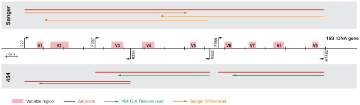
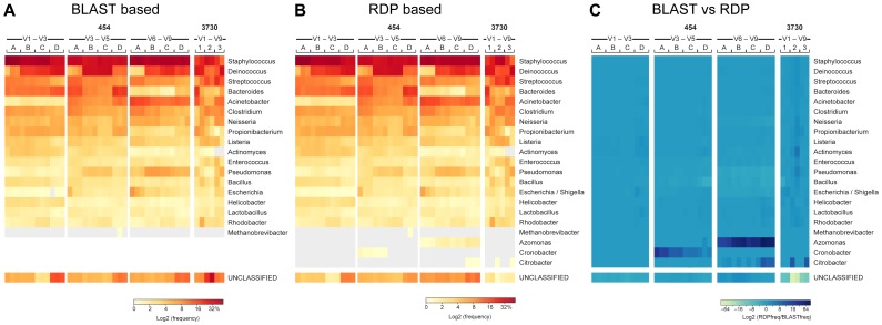
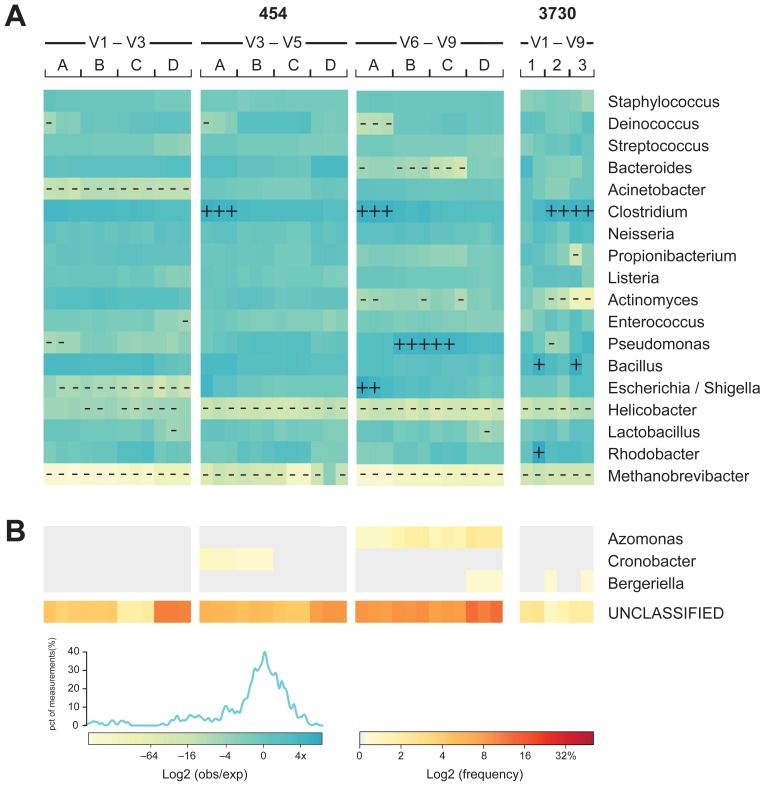
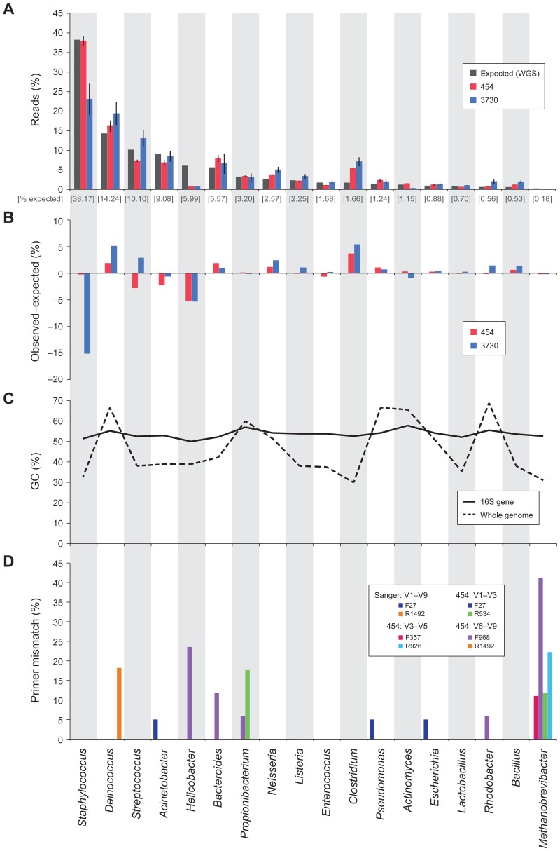
The Human Microbiome Project will establish a reference data set for analysis of the microbiome of healthy adults by surveying multiple body sites from 300 people and generating data from over 12,000 samples. To characterize these samples, the participating sequencing centers evaluated and adopted 16S rDNA community profiling protocols for ABI 3730 and 454 FLX Titanium sequencing. In the course of establishing protocols, we examined the performance and error characteristics of each technology, and the relationship of sequence error to the utility of 16S rDNA regions for classification- and OTU-based analysis of community structure. The data production protocols used for this work are those used by the participating centers to produce 16S rDNA sequence for the Human Microbiome Project. Thus, these results can be informative for interpreting the large body of clinical 16S rDNA data produced for this project.
Overview
The claims and statistics of this paper haven’t been checked yet.
Run the check — free, no account needed. It reads the open-access text and checks the sources it cites.
Integrity signals
Registry
Cites
Statistics
Figures
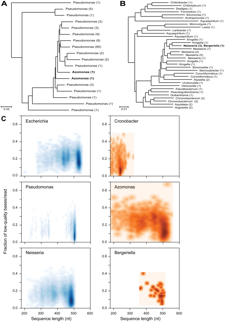
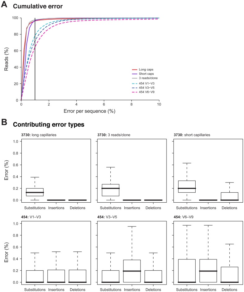
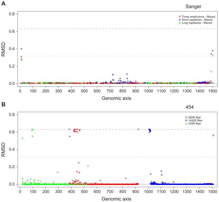
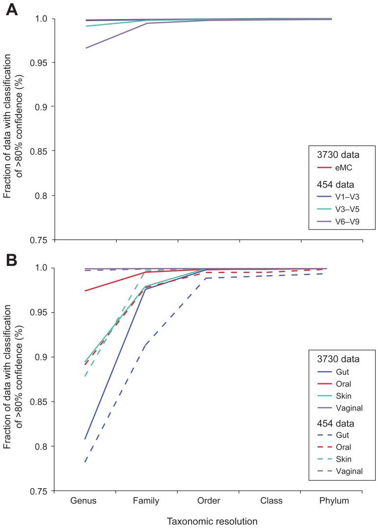
Verification
Claims the paper makes
The claims and statistics of this paper haven’t been checked yet.
Run the check — free, no account needed. It reads the open-access text and checks the sources it cites.
Claims other papers make about this one
Each is checked against this paper’s own text: does it say what the citing paper says it does?
In the citing paper
“Inter-study technical variability in microbiome measurements can sometimes, for example, outweigh biological effects6–9.”
From Assessment of variation in microbial community amplicon sequencing by the Microbiome Quality Control (MBQC) project consortium (2017) · cites this paper as [7]
In the citing paper
“DNA extraction protocols are a known source of variation between microbial community characterization experiments7–9.”
From Assessment of variation in microbial community amplicon sequencing by the Microbiome Quality Control (MBQC) project consortium (2017) · cites this paper as [7]
Self-check
Percentages, sums and reported differences re-computed from the paper’s own numbers.
The self-check needs the paper’s full text.
Citations
Cites
The Sequence Alignment/Map format and SAMtools
Li, H., Handsaker, B., Wysoker, A., Fennell, T., Ruan, J., Homer, N., Marth, G., Abecasis, G., Durbin, R., & 1000 Genome Project Data Processing Subgroup (2009) · Bioinformatics · doi:10.1093/bioinformatics/btp352 · Cited by 62,041
Fast and accurate short read alignment with Burrows-Wheeler transform
Li, H., & Durbin, R. (2009) · Bioinformatics · doi:10.1093/bioinformatics/btp324 · Cited by 58,607
Naive Bayesian Classifier for Rapid Assignment of rRNA Sequences into the New Bacterial Taxonomy
Wang, Q., Garrity, G. M., Tiedje, J. M., & Cole, J. R. (2007) · Applied and Environmental Microbiology · doi:10.1128/aem.00062-07 · Cited by 20,145
Schloss, P. D., Westcott, S. L., Ryabin, T., Hall, J. R., Hartmann, M., Hollister, E. B., Lesniewski, R. A., Oakley, B. B., Parks, D. H., Robinson, C. J., et al. (2009) · Applied and Environmental Microbiology · doi:10.1128/aem.01541-09 · Cited by 19,549
Global patterns of 16S rRNA diversity at a depth of millions of sequences per sample
Caporaso, J. G., Lauber, C. L., Walters, W. A., Berg-Lyons, D., Lozupone, C., Turnbaugh, P. J., Fierer, N., & Knight, R. D. (2010) · Proceedings of the National Academy of Sciences · doi:10.1073/pnas.1000080107 · Cited by 9,944
A core gut microbiome in obese and lean twins
Turnbaugh, P. J., Hamady, M., Yatsunenko, T., Cantarel, B. L., Duncan, A., Ley, R. E., Sogin, M. L., Jones, W. J., Roe, B. A., Affourtit, J. P., et al. (2009) · Nature · doi:10.1038/nature07540 · Cited by 7,823
Vaginal microbiome of reproductive-age women
Ravel, J., Gajer, P., Abdo, Z., Schneider, G. M., Koenig, S. S. K., McCulle, S. L., Karlebach, S., Gorle, R., Russell, J., Tacket, C. O., et al. (2011) · Proceedings of the National Academy of Sciences · doi:10.1073/pnas.1002611107 · Cited by 4,254
Chimeric 16S rRNA sequence formation and detection in Sanger and 454-pyrosequenced PCR ampliconsPreprint
Haas, B. J., Gevers, D., Earl, A. M., Feldgarden, M., Ward, D. V., Giannoukos, G., Ciulla, D., Tabbaa, D., Highlander, S. K., Sodergren, E. J., et al. (2011) · Genome Research · doi:10.1101/gr.112730.110 · Cited by 3,527
Bacterial Community Variation in Human Body Habitats Across Space and Time
Costello, E. K., Lauber, C. L., Hamady, M., Fierer, N., Gordon, J. I., & Knight, R. (2009) · Science · doi:10.1126/science.1177486 · Cited by 3,231
Topographical and Temporal Diversity of the Human Skin Microbiome
Grice, E. A., Kong, H. H., Conlan, S., Deming, C. B., Davis, J., Young, A. C., Program, N. C. S., Bouffard, G. G., Blakesley, R. W., Murray, P. R., et al. (2009) · Science · doi:10.1126/science.1171700 · Cited by 2,953
Cited by
Sorted by citations
Microbial interactions: from networks to models
Faust, K., & Raes, J. (2012) · Nature Reviews Microbiology · doi:10.1038/nrmicro2832 · Cited by 4,268
Inferring Correlation Networks from Genomic Survey Data
Friedman, J., & Alm, E. J. (2012) · PLoS Computational Biology · doi:10.1371/journal.pcbi.1002687 · Cited by 2,765
A framework for human microbiome research
The Human Microbiome Project Consortium (2012) · Nature · doi:10.1038/nature11209 · Cited by 2,650
Best practices for analysing microbiomes
Knight, R., Vrbanac, A., Taylor, B. C., Aksenov, A., Callewaert, C., Debelius, J., Gonzalez, A., Kosciolek, T., McCall, L.-I., McDonald, D., et al. (2018) · Nature Reviews Microbiology · doi:10.1038/s41579-018-0029-9 · Cited by 2,030
The Integrative Human Microbiome Project
The Integrative HMP (iHMP) Research Network Consortium, Proctor, L. M., Creasy, H. H., Fettweis, J. M., Lloyd-Price, J., Mahurkar, A., Zhou, W., Buck, G. A., Snyder, M. P., Strauss, J. F., et al. (2019) · Nature · doi:10.1038/s41586-019-1238-8 · Cited by 1,381
Biogeography and individuality shape function in the human skin metagenome
Program, N. C. S., Oh, J., Byrd, A. L., Deming, C., Conlan, S., Kong, H. H., & Segre, J. A. (2014) · Nature · doi:10.1038/nature13786 · Cited by 1,148
Dynamics and associations of microbial community types across the human body
Ding, T., & Schloss, P. D. (2014) · Nature · doi:10.1038/nature13178 · Cited by 885
Systematic improvement of amplicon marker gene methods for increased accuracy in microbiome studies
Gohl, D. M., Vangay, P., Garbe, J., Maclean, A., Hauge, A., Becker, A., Gould, T. J., Clayton, J. B., Johnson, T. J., Hunter, R. C., et al. (2016) · Nature Biotechnology · doi:10.1038/nbt.3601 · Cited by 834
Biogeography of the ecosystems of the healthy human body
Zhou, Y., Gao, H., Mihindukulasuriya, K. A., Rosa, P. S. L., Wylie, K. M., Vishnivetskaya, T. A., Podar, M., Warner, B., Tarr, P. I., Nelson, D. E., et al. (2013) · Genome biology · doi:10.1186/gb-2013-14-1-r1 · Cited by 689
Machine Learning Meta-analysis of Large Metagenomic Datasets: Tools and Biological Insights
Pasolli, E., Truong, D. T., Malik, F., Waldron, L., & Segata, N. (2016) · PLOS Computational Biology · doi:10.1371/journal.pcbi.1004977 · Cited by 659
An introduction to the analysis of shotgun metagenomic data
Sharpton, T. J. (2014) · Frontiers in Plant Science · doi:10.3389/fpls.2014.00209 · Cited by 708
“Advances in laboratory procedures that physically separate microbiota from plant tissue (e.g., Jiao et al., 2006; Delmotte et al., 2009) will continue to improve the efficacy of metagenomic investigations in plant systems.”
BackgroundFunGene: the functional gene pipeline and repository
Fish, J. A., Chai, B., Wang, Q., Sun, Y., Brown, C. T., Tiedje, J. M., & Cole, J. R. (2013) · Frontiers in Microbiology · doi:10.3389/fmicb.2013.00291 · Cited by 646
The Microbiome Quality Control Project Consortium, Sinha, R., Abu-Ali, G., Vogtmann, E., Fodor, A. A., Ren, B., Amir, A., Schwager, E., Crabtree, J., Ma, S., et al. (2017) · Nature Biotechnology · doi:10.1038/nbt.3981 · Cited by 587
The truth about metagenomics: quantifying and counteracting bias in 16S rRNA studies
Vaginal Microbiome Consortium (additional members), Brooks, J. P., Edwards, D. J., Harwich, M. D., Rivera, M. C., Fettweis, J. M., Serrano, M. G., Reris, R. A., Sheth, N. U., Huang, B., et al. (2015) · BMC Microbiology · doi:10.1186/s12866-015-0351-6 · Cited by 528
Koren, O., Knights, D., Gonzalez, A., Waldron, L., Segata, N., Knight, R., Huttenhower, C., & Ley, R. E. (2013) · PLoS Computational Biology · doi:10.1371/journal.pcbi.1002863 · Cited by 508
Bull–Otterson, L., Feng, W., Kirpich, I., Wang, Y., Qin, X., Liu, Y., Gobejishvili, L., Joshi‐Barve, S., Ayvaz, T., Petrosino, J. F., et al. (2013) · PLoS ONE · doi:10.1371/journal.pone.0053028 · Cited by 553
Genomic approaches to studying the human microbiota
Weinstock, G. M. (2012) · Nature · doi:10.1038/nature11553 · Cited by 558
Primer and platform effects on 16S rRNA tag sequencing
Tremblay, J., Singh, K. P., Fern, A., Kirton, E., He, S., Woyke, T., Lee, J., Chen, F., Dangl, J. L., & Tringe, S. G. (2015) · Frontiers in Microbiology · doi:10.3389/fmicb.2015.00771 · Cited by 549
Albertsen, M., Karst, S. M., Ziegler, A., Kirkegaard, R. H., & Nielsen, P. H. (2015) · PLoS ONE · doi:10.1371/journal.pone.0132783 · Cited by 540
The Human Microbiome Project: A Community Resource for the Healthy Human Microbiome
Gevers, D., Knight, R., Petrosino, J. F., Huang, K., McGuire, A. L., Birren, B. W., Nelson, K. E., White, O., Methé, B. A., & Huttenhower, C. (2012) · PLoS Biology · doi:10.1371/journal.pbio.1001377 · Cited by 493
Primer, Pipelines, Parameters: Issues in 16S rRNA Gene Sequencing
Abellan-Schneyder, I., Matchado, M. S., Reitmeier, S., Sommer, A., Sewald, Z., Baumbach, J., List, M., & Neuhaus, K. (2021) · mSphere · doi:10.1128/msphere.01202-20 · Cited by 542
Use of 16S rRNA Gene for Identification of a Broad Range of Clinically Relevant Bacterial Pathogens
Srinivasan, R., Karaöz, U., Volegova, M. P., MacKichan, J. K., Kato‐Maeda, M., Miller, S. A., Nadarajan, R., Brodie, E., & Lynch, S. V. (2015) · PLoS ONE · doi:10.1371/journal.pone.0117617 · Cited by 508
The role of the gut microbiome in the healthy adult status
D’Argenio, V., & Salvatore, F. (2015) · Clinica Chimica Acta · doi:10.1016/j.cca.2015.01.003 · Cited by 492
Community differentiation of the cutaneous microbiota in psoriasis
Alekseyenko, A. V., Perez-Perez, G. I., Souza, A. D., Strober, B. E., Gao, Z., Bihan, M., Li, K., Methé, B. A., & Blaser, M. J. (2013) · Microbiome · doi:10.1186/2049-2618-1-31 · Cited by 454
The role of the intestinal microbiota in type 1 diabetes mellitus
Knip, M., & Siljander, H. (2016) · Nature Reviews Endocrinology · doi:10.1038/nrendo.2015.218 · Cited by 444
Han, M. K., Zhou, Y., Murray, S., Tayob, N., Noth, I., Lama, V. N., Moore, B. B., White, E. S., Flaherty, K. R., Hu, B., et al. (2014) · The Lancet Respiratory Medicine · doi:10.1016/s2213-2600(14)70069-4 · Cited by 419
Greenwood, C., Morrow, A. L., Lagomarcino, A. J., Altaye, M., Taft, D. H., Yu, Z., Newburg, D. S., Ward, D. V., & Schibler, K. R. (2014) · The Journal of Pediatrics · doi:10.1016/j.jpeds.2014.01.010 · Cited by 416
Structure and function of the healthy pre-adolescent pediatric gut microbiome
Hollister, E. B., Riehle, K., Luna, R. A., Weidler, E. M., Rubio-Gonzales, M., Mistretta, T.-A., Raza, S., Doddapaneni, H. V., Metcalf, G. A., Muzny, D. M., et al. (2015) · Microbiome · doi:10.1186/s40168-015-0101-x · Cited by 406
Relationship between the gut microbiome and brain function
Mohajeri, M. H., La Fata, G., Steinert, R. E., & Weber, P. (2018) · Nutrition Reviews · doi:10.1093/nutrit/nuy009 · Cited by 376
Said, H. S., Suda, W., Nakagome, S., Chinen, H., Oshima, K., Kim, S., Kimura, R., Iraha, A., Ishida, H., Fujita, J., et al. (2013) · DNA Research · doi:10.1093/dnares/dst037 · Cited by 394
Host genetics and the rumen microbiome jointly associate with methane emissions in dairy cows
Difford, G. F., Plichta, D. R., Løvendahl, P., Lassen, J., Noel, S. J., Højberg, O., Wright, A. G., Zhu, Z., Kristensen, L., Nielsen, H. B., et al. (2018) · PLoS Genetics · doi:10.1371/journal.pgen.1007580 · Cited by 404
“Universal bacterial 16S rRNA gene primers (covering the V1-V3 variable regions) 27F: 5’-AGAGTTTGATCCTGGCTCAG-3’ and 534R: 5’-ATTACCGCGGCTGCTG G-3’ were used to generate the bacterial amplicon libraries (expected amplicon size 508 bp) [74].”
MethodAagaard, K., Petrosino, J., Keitel, W., Watson, M., Katancik, J., Garcia, N., Patel, S., Cutting, M., Madden, T., Hamilton, H., et al. (2013) · The FASEB Journal · doi:10.1096/fj.12-220806 · Cited by 383
The human mycobiome in health and disease
Cui, L., Morris, A., & Ghedin, E. (2013) · Genome Medicine · doi:10.1186/gm467 · Cited by 394
Morrow, A. L., Lagomarcino, A. J., Schibler, K. R., Taft, D. H., Yu, Z., Wang, B., Altaye, M., Wagner, M., Gevers, D., Ward, D. V., et al. (2013) · Microbiome · doi:10.1186/2049-2618-1-13 · Cited by 350
“The V3 to V5 window of the 16S rRNA gene was amplified and sequenced using 454 FLX Titanium sequencing as already described in full detail [32].”
MethodThe gut-brain axis: the missing link in depression
Evrensel, A., & Ceylan, M. E. (2015) · Clinical Psychopharmacology and Neuroscience · doi:10.9758/cpn.2015.13.3.239 · Cited by 338
Diversity of the Vaginal Microbiome Correlates With Preterm Birth
Hyman, R. W., Fukushima, M., Jiang, H., Fung, E., Rand, L., Johnson, B., Vo, K. C., Caughey, A. B., Hilton, J. F., Davis, R. W., et al. (2013) · Reproductive Sciences · doi:10.1177/1933719113488838 · Cited by 340
Skin Microbiome Surveys Are Strongly Influenced by Experimental Design
Meisel, J. S., Hannigan, G. D., Tyldsley, A. S., SanMiguel, A. J., Hodkinson, B. P., Zheng, Q., & Grice, E. A. (2016) · Journal of Investigative Dermatology · doi:10.1016/j.jid.2016.01.016 · Cited by 330
Metagenomic analysis of size-fractionated picoplankton in a marine oxygen minimum zone
Ganesh, S., Parris, D. J., DeLong, E. F., & Stewart, F. J. (2013) · The ISME Journal · doi:10.1038/ismej.2013.144 · Cited by 324
Analysis, Optimization and Verification of Illumina-Generated 16S rRNA Gene Amplicon Surveys
Nelson, M. C., Morrison, H. G., Benjamino, J., Grim, S. L., & Graf, J. (2014) · PLoS ONE · doi:10.1371/journal.pone.0094249 · Cited by 339
Guerrero-Preston, R. E., Godoy‐Vitorino, F., Jedlicka, A., Rodríguez-Hilario, A., González, H., Bondy, J., Lawson, F. P., Folawiyo, O., Michailidi, C., Dziedzic, A., et al. (2016) · Oncotarget · doi:10.18632/oncotarget.9710 · Cited by 322
“…gene has nine variable regions: a combination of variable and moderately conserved regions is optimal for performing analyses at different phylogenetic depths, and the V3-V5 region is one of the preferred regions for characterizing the communities with few errors for taxonomy assignment [20-22].”
Scales, B. S., Dickson, R. P., LiPuma, J. J., & Huffnagle, G. B. (2014) · Clinical Microbiology Reviews · doi:10.1128/cmr.00044-14 · Cited by 325
Boers, S. A., Jansen, R., & Hays, J. P. (2019) · European Journal of Clinical Microbiology & Infectious Diseases · doi:10.1007/s10096-019-03520-3 · Cited by 297
The bovine milk microbiota: insights and perspectives from -omics studies
Addis, M. F., Tanca, A., Uzzau, S., Oikonomou, G., Bicalho, R. C., & Moroni, P. (2016) · Molecular BioSystems · doi:10.1039/c6mb00217j · Cited by 297
West, C. E., Renz, H. E., Jenmalm, M. C., Kozyrskyj, A. L., Allen, K. J., Vuillermin, P., Prescott, S. L., Mackay, C. R., Salminen, S., Wong, G., et al. (2015) · Journal of Allergy and Clinical Immunology · doi:10.1016/j.jaci.2014.11.012 · Cited by 288
Early pregnancy vaginal microbiome trends and preterm birth
Stout, M. J., Zhou, Y., Wylie, K. M., Tarr, P. I., Macones, G. A., & Tuuli, M. G. (2017) · American Journal of Obstetrics and Gynecology · doi:10.1016/j.ajog.2017.05.030 · Cited by 269
Labus, J. S., Hollister, E. B., Jacobs, J., Kirbach, K., Oezguen, N., Gupta, A., Acosta, J., Luna, R. A., Aagaard, K., Versalovic, J., et al. (2017) · Microbiome · doi:10.1186/s40168-017-0260-z · Cited by 284
Host Response to the Lung Microbiome in Chronic Obstructive Pulmonary Disease
Sze, M. A., Dimitriu, P. A., Suzuki, M., McDonough, J. E., Campbell, J. D., Brothers, J. F., Erb‐Downward, J. R., Huffnagle, G. B., Hayashi, S., Elliott, W. M., et al. (2015) · American Journal of Respiratory and Critical Care Medicine · doi:10.1164/rccm.201502-0223oc · Cited by 260
Data analysis for 16S microbial profiling from different benchtop sequencing platforms
Pylro, V. S., Roesch, L. F. W., Morais, D., Clark, I. M., Hirsch, P. R., & Tótola, M. R. (2014) · Journal of Microbiological Methods · doi:10.1016/j.mimet.2014.08.018 · Cited by 247
Bacterial Communities of the Coronal Sulcus and Distal Urethra of Adolescent Males
Nelson, D. E., Dong, Q., Pol, B. J. V. D., Toh, E. C., Fan, B., Katz, B. P., Mi, D., Rong, R., Weinstock, G. M., Sodergren, E. J., et al. (2012) · PLoS ONE · doi:10.1371/journal.pone.0036298 · Cited by 242
Analysis of soil microbial communities based on amplicon sequencing of marker genes
Schöler, A., Jacquiod, S., Vestergaard, G., Schulz, S., & Schloter, M. (2017) · Biology and Fertility of Soils · doi:10.1007/s00374-017-1205-1 · Cited by 237
Performing Skin Microbiome Research: A Method to the Madness
Kong, H. H., Andersson, B., Clavel, T., Common, J., Jackson, S. A., Olson, N. D., Segre, J. A., & Traidl‐Hoffmann, C. (2017) · Journal of Investigative Dermatology · doi:10.1016/j.jid.2016.10.033 · Cited by 232
Combining 16S rRNA gene variable regions enables high-resolution microbial community profiling
(2017) · doi:10.1186/s40168-017-0396-x · Cited by 266
“All species were detected in both regions, apart from Methanobrevibacter which neither regions amplified [34].”
BackgroundThe Dental Plaque Microbiome in Health and Disease
Peterson, S. N., Snesrud, E. C., Liu, J., Ong, A., Kilian, M., Schork, N. J., & Bretz, W. A. (2013) · PLoS ONE · doi:10.1371/journal.pone.0058487 · Cited by 227
“This composition is consistent with data generated as part of the HMP consortium surveys [34–36].”
ResultReference standards for next-generation sequencing
Hardwick, S. A., Deveson, I. W., & Mercer, T. R. (2017) · Nature Reviews Genetics · doi:10.1038/nrg.2017.44 · Cited by 227
Capturing the diversity of the human gut microbiota through culture-enriched molecular profiling
Lau, J. Y. F., Whelan, F., Herath, I., Lee, C., Collins, S. M., Berčík, P., & Surette, M. G. (2016) · Genome Medicine · doi:10.1186/s13073-016-0327-7 · Cited by 229
Tick microbiome and pathogen acquisition altered by host blood meal
Swei, A., & Kwan, J. Y. (2016) · The ISME Journal · doi:10.1038/ismej.2016.152 · Cited by 207
Ramiro‐Garcia, J., Hermes, G. D. A., Giatsis, C., Sipkema, D., Zoetendal, E. G., Schaap, P. J., & Smidt, H. (2016) · F1000Research · doi:10.12688/f1000research.9227.2 · Cited by 238
The antipsychotic olanzapine interacts with the gut microbiome to cause weight gain in mouse
Morgan, A. P., Crowley, J. J., Nonneman, R. J., Quackenbush, C. R., Miller, C. N., Ryan, A. K., Bogue, M. A., Paredes, S. H., Yourstone, S., Carroll, I. M., et al. (2014) · PLoS ONE · doi:10.1371/journal.pone.0115225 · Cited by 197
Lluch, J., Servant, F., Païssé, S., Valle, C., Valière, S., Kuchly, C., Vilchez, G., Donnadieu, C., Courtney, M., Burcelin, R., et al. (2015) · PLoS ONE · doi:10.1371/journal.pone.0142334 · Cited by 195
Chu, D. M., Meyer, K. M., Prince, A., & Aagaard, K. M. (2016) · Gut Microbes · doi:10.1080/19490976.2016.1241357 · Cited by 188
Harnessing Gut Microbes for Mental Health: Getting From Here to There
Bruce‐Keller, A. J., Salbaum, J. M., & Berthoud, H. (2017) · Biological Psychiatry · doi:10.1016/j.biopsych.2017.08.014 · Cited by 192
Pregnancy's Stronghold on the Vaginal Microbiome
Walther-Antonio, M. R. S., Jeraldo, P., Miller, M. E. B., Yeoman, C. J., Nelson, K. E., Wilson, B. A., White, B. A., Chia, N., & Creedon, D. J. (2014) · PLoS ONE · doi:10.1371/journal.pone.0098514 · Cited by 187
Ramiro‐Garcia, J., Hermes, G. D. A., Giatsis, C., Sipkema, D., Zoetendal, E. G., Schaap, P. J., & Smidt, H. (2016) · F1000Research · doi:10.12688/f1000research.9227.1 · Cited by 187
MixMC: A Multivariate Statistical Framework to Gain Insight into Microbial Communities
Cao, K. L., Costello, M., Lakis, V., Bartolo, F., Chua, X., Brazeilles, R., & Rondeau, P. (2016) · PLoS ONE · doi:10.1371/journal.pone.0160169 · Cited by 188
“While many published analyses have focused on the main microbial habitats (gut, oral cavity, skin and vagina from the [24, 47]), little has been done to comprehensively characterise multiple sites within a single habitat.”
BackgroundMeta'omic Analytic Techniques for Studying the Intestinal Microbiome
Morgan, X. C., & Huttenhower, C. (2014) · Gastroenterology · doi:10.1053/j.gastro.2014.01.049 · Cited by 181
Survival in hostile territory: the microbiota of the stomach
Yang, I., Nell, S., & Suerbaum, S. (2013) · FEMS Microbiology Reviews · doi:10.1111/1574-6976.12027 · Cited by 168
SPINGO: a rapid species-classifier for microbial amplicon sequences
Allard, G., Ryan, F. J., Jeffery, I. B., & Claesson, M. J. (2015) · BMC Bioinformatics · doi:10.1186/s12859-015-0747-1 · Cited by 156
“Variable regions V1-V3 (6,046 sequences), V3-V5 (5,860) and V6-V9 (5,241) were extracted from the SILVA database using previously described primers [11] with the V-ripper script and subsequently classified using the evaluation database not containing the 9,607 test sequences.”
MethodMicrobial phylogenetic profiling with the Pacific Biosciences sequencing platform
Fichot, E. B., & Norman, R. S. (2013) · Microbiome · doi:10.1186/2049-2618-1-10 · Cited by 161
Kubinak, J. L., Stephens, W. Z., Soto, R., Petersen, C., Chiaro, T. R., Gogokhia, L., Bell, R. S., Ajami, N. J., Petrosino, J. F., Morrison, L. C., et al. (2015) · Nature Communications · doi:10.1038/ncomms9642 · Cited by 157
“The 16S rRNA gene libraries were generated by the Center for Metagenomics and Microbiome Research at Baylor College of Medicine, using the V3-V5 (357F/926R) primer in accordance with standard HMP protocols 50 .”
Oulhen, N., Schulz, B., & Carrier, T. J. (2016) · Symbiosis · doi:10.1007/s13199-016-0409-8 · Cited by 158
Modulation of the faecal microbiome of healthy adult dogs by inclusion of potato fibre in the diet
Panasevich, M. R., Kerr, K. R., Dilger, R. N., Fahey, G. C., Jr., Guérin‐Deremaux, L., Lynch, G. L., Wils, D., Suchodolski, J. S., Steer, J. M., Dowd, S. E., et al. (2014) · British Journal Of Nutrition · doi:10.1017/s0007114514003274 · Cited by 166
Impact of Preservation Method and 16S rRNA Hypervariable Region on Gut Microbiota Profiling
Chen, Z., Hui, P. C., Hui, M., Yeoh, Y. K., Wong, P. Y., Chan, M. C. W., Wong, M. C. S., Ng, S. C., Chan, F. K. L., & Chan, P. K. S. (2019) · mSystems · doi:10.1128/msystems.00271-18 · Cited by 160
Mukherjee, S., Mitra, R., Maitra, A., Gupta, S., Kumaran, S., Chakrabortty, A., & Majumder, P. P. (2016) · Scientific Reports · doi:10.1038/srep36062 · Cited by 153
Tiny microbes, enormous impacts: what matters in gut microbiome studies?
Debelius, J. W., Song, S. J., Vázquez‐Baeza, Y., Xu, Z. Z., González, A., & Knight, R. D. (2016) · Genome biology · doi:10.1186/s13059-016-1086-x · Cited by 160
Ancient DNA analysis of dental calculus
Weyrich, L. S., Dobney, K., & Cooper, A. (2015) · Journal of Human Evolution · doi:10.1016/j.jhevol.2014.06.018 · Cited by 147
Lohmann, P., Luna, R. A., Hollister, E. B., Devaraj, S., Mistretta, T.-A., Welty, S. E., & Versalovic, J. (2014) · Pediatric Research · doi:10.1038/pr.2014.85 · Cited by 146
Urinary Microbiome and Cytokine Levels in Women With Interstitial Cystitis
Abernethy, M., Rosenfeld, A. B., White, J. R., Mueller, M. G., Lewicky‐Gaupp, C., & Kenton, K. S. (2017) · Obstetrics and Gynecology · doi:10.1097/aog.0000000000001892 · Cited by 135
The Perinatal Microbiome and Pregnancy: Moving Beyond the Vaginal MicrobiomePreprint
Prince, A., Chu, D. M., Seferovic, M., Antony, K. M., Ma, J., & Aagaard, K. M. (2015) · Cold Spring Harbor Perspectives in Medicine · doi:10.1101/cshperspect.a023051 · Cited by 141
Yooseph, S., Kirkness, E. F., Tran, T. M., Harkins, D. M., Jones, M. B., Torralba, M., O’Connell, E. M., Nutman, T. B., Doumbo, S., Doumbo, O. K., et al. (2015) · BMC Genomics · doi:10.1186/s12864-015-1819-3 · Cited by 131
Nyyssönen, M., Hultman, J., Ahonen, L., Kukkonen, I., Paulin, L. G., Laine, P., Itävaara, M., & Auvinen, P. (2013) · The ISME Journal · doi:10.1038/ismej.2013.125 · Cited by 133
“This can result in differences in taxonomic resolution (Ward et al., 2012).”
BackgroundBarb, J. J., Oler, A. J., Kim, H., Chalmers, N. I., Wallen, G. R., Cashion, A. K., Munson, P. J., & Ames, N. J. (2016) · PLoS ONE · doi:10.1371/journal.pone.0148047 · Cited by 133
Hardwick, S. A., Chen, W. Y., Wong, T., Madala, B. S., Deveson, I. W., Ongley, S. E., Santini, N. S., Marcellin, E., Smith, M. A., Nielsen, L. K., et al. (2018) · Nature Communications · doi:10.1038/s41467-018-05555-0 · Cited by 134
Fecal Microbiota Analysis: An Overview of Sample Collection Methods and Sequencing Strategies
Thomas, V., Clark, J. R., & Dore, J. M. (2015) · Future Microbiology · doi:10.2217/fmb.15.87 · Cited by 138
Next generation sequencing data of a defined microbial mock community
Singer, E., Andreopoulos, B., Bowers, R. M., Lee, J., Deshpande, S., Chiniquy, J., Ciobanu, D., Klenk, H., Zane, M., Daum, C. G., et al. (2016) · Scientific Data · doi:10.1038/sdata.2016.81 · Cited by 115
Metagenomic Surveys of Gut Microbiota
Mandal, R. S., Saha, S., & Das, S. (2015) · Genomics Proteomics & Bioinformatics · doi:10.1016/j.gpb.2015.02.005 · Cited by 123
What Is Metagenomics Teaching Us, and What Is Missed?
New, F. N., & Brito, I. (2020) · Annual Review of Microbiology · doi:10.1146/annurev-micro-012520-072314 · Cited by 124
Oral Microbiome of Deep and Shallow Dental Pockets In Chronic Periodontitis
Ge, X., Rodriguez, R., Trinh, M., Gunsolley, J. C., & Xu, P. (2013) · PLoS ONE · doi:10.1371/journal.pone.0065520 · Cited by 118
Corsino, S. F., Capodici, M., Pippo, F. D., Tandoi, V., & Torregrossa, M. (2018) · Water Research · doi:10.1016/j.watres.2018.10.086 · Cited by 113
Stehlikova, Z., Kostovcik, M., Kostovcikova, K., Kverka, M., Juzlova, K., Rob, F., Hercogova, J., Bohac, P., Pinto, Y., Uzan, A., et al. (2019) · Frontiers in Microbiology · doi:10.3389/fmicb.2019.00438 · Cited by 105
Bahrndorff, S., de Jonge, N., Skovgård, H., & Nielsen, J. L. (2017) · PLoS ONE · doi:10.1371/journal.pone.0169753 · Cited by 108
Park, H., Shin, J. W., Park, S.-G., & Kim, W. (2014) · PLoS ONE · doi:10.1371/journal.pone.0109710 · Cited by 101
IM-TORNADO: A Tool for Comparison of 16S Reads from Paired-End Libraries
Jeraldo, P., Kalari, K. R., Chen, X., Bhavsar, J., Mangalam, A. K., White, B. A., Nelson, H., Kocher, J.-P. A., & Chia, N. (2014) · PLoS ONE · doi:10.1371/journal.pone.0114804 · Cited by 99
Guerrero-Preston, R. E., White, J. R., Godoy‐Vitorino, F., Rodríguez-Hilario, A., Navarro, K., González, H., Michailidi, C., Jedlicka, A., Canapp, S., Bondy, J., et al. (2017) · Oncotarget · doi:10.18632/oncotarget.20677 · Cited by 98
Wind and sunlight shape microbial diversity in surface waters of the North Pacific Subtropical Gyre
Bryant, J. A., Aylward, F. O., Eppley, J. M., Karl, D. M., Church, M. J., & DeLong, E. F. (2015) · The ISME Journal · doi:10.1038/ismej.2015.221 · Cited by 104
Kirpich, I., Petrosino, J. F., Ajami, N. J., Feng, W., Wang, Y., Liu, Y., Beier, J. I., Barve, S. S., Yin, X., Wei, X., et al. (2016) · American Journal Of Pathology · doi:10.1016/j.ajpath.2015.11.017 · Cited by 96
Rago, L., Ruiz, Y., Baeza, J. A., Guisasola, A., & Cortés, P. (2015) · Bioelectrochemistry · doi:10.1016/j.bioelechem.2015.06.003 · Cited by 92
Bioinformatics for the Human Microbiome Project
Gevers, D., Pop, M., Schloss, P. D., & Huttenhower, C. (2012) · PLoS Computational Biology · doi:10.1371/journal.pcbi.1002779 · Cited by 91
Wang, J., Tang, L., Zhou, J., Zhou, J., Glenn, T. C., Shen, C., & Wang, J.-S. (2018) · The Journal of Nutritional Biochemistry · doi:10.1016/j.jnutbio.2018.01.005 · Cited by 90
The vaginal eukaryotic DNA virome and preterm birth
Wylie, K. M., Wylie, T., Cahill, A. G., Macones, G. A., Tuuli, M. G., & Stout, M. J. (2018) · American Journal of Obstetrics and Gynecology · doi:10.1016/j.ajog.2018.04.048 · Cited by 91
Myer, P. R., Kim, M., Freetly, H. C., & Smith, T. P. L. (2016) · Journal of Microbiological Methods · doi:10.1016/j.mimet.2016.06.004 · Cited by 88
Metadata
- Authors
- Jumpstart Consortium Human Microbiome Project Data Generation Working Group
- Affiliations
- University of Maryland, Baltimore (US)
- Corresponding author
- Jumpstart Consortium Human Microbiome Project Data Generation Working Group
- Venue
- PLoS ONE
- Publisher
- Public Library of Science (PLoS)
- Published
- 2012-06-13
- Volume
- 7
- Issue
- 6
- Pages
- e39315
- ISSN
- 1932-6203 (ISSN-L)
- PMC
- PMC3374619
- OpenAlex
- W2319405466
- Cited by
- 297
- References
- 38
- Citations by year
- 2026: 2 · 2025: 5 · 2024: 5 · 2023: 8 · 2022: 6 · 2021: 22 · 2020: 17 · 2019: 27 · 2018: 22 · 2017: 35 · 2016: 31 · 2015: 39 · 2014: 31 · 2013: 34 · 2012: 12
- FWCI
- 14.90
- Type
- journal article
- Language
- en
- Open access
- gold
- doi.org
- Locations
- PLoS ONE (publishedVersion, cc-by)
- PubMed Central (publishedVersion, cc-by)
- PubMed (publishedVersion)
- DOAJ (DOAJ: Directory of Open Access Journals) (submittedVersion)
- Figshare (submittedVersion, cc-by)
- Funders
- Broad Institute
- National Institutes of Health
- U.S. Public Health Service (HHSN2722009000018C)
- National Human Genome Research Institute (U54HG004969, U54HG003079, U01HG004866, U54HG003273, U54HG004968, U54HG004973)
- National Institute of Allergy and Infectious Diseases (HHSN272200900018C, HHSN272200900001C, HHSN272200900008C, U54AI084844)
- Topics
- Life Sciences › Biochemistry, Genetics and Molecular Biology › Molecular Biology › Genomics and Phylogenetic Studies
- Life Sciences › Biochemistry, Genetics and Molecular Biology › Molecular Biology › Gut microbiota and health
- Physical Sciences › Environmental Science › Ecology › Microbial Community Ecology and Physiology
- Keywords
- 16S rRNA gene, human microbiome, Human Microbiome Project, sequencing errors, community structure, reference dataset
- MeSH terms
- Bacteria, Bayes Theorem, Humans, RNA, Ribosomal, 16S, Metagenome
About these checks
Registry, retraction, Cites and statistics results are computed, not judged, with one exception: a printed reference that no index lists is read once by a model before it counts as a citation error. Claims are extracted by a model and kept only when their quote appears verbatim in the text; each cited source is then checked, with a model’s help, for whether it says what the claim relies on. Those verdicts can be wrong — read the claim’s quote and the cited source before relying on one.
Statistics and arithmetic are recomputed, not judged.
Confidence bands are shown only for fields calibrated on our annotated test set. None is calibrated yet, so no band is shown.
What counts as a claim ›How we measure confidence ›How we check this ›
Are you an author, or do you see a problem with this page? Request a review
