

The DOI matches its Crossref record; 52 of the 53 references it cites were found in a registry or an index; 3 of the 37 sources its claims cite were checked for support.
Multiscale 3D Genome Rewiring during Mouse Neural Development
Open accessAbstract
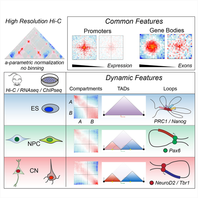
Chromosome conformation capture technologies have revealed important insights into genome folding. Yet, how spatial genome architecture is related to gene expression and cell fate remains unclear. We comprehensively mapped 3D chromatin organization during mouse neural differentiation in vitro and in vivo, generating the highest-resolution Hi-C maps available to date. We found that transcription is correlated with chromatin insulation and long-range interactions, but dCas9-mediated activation is insufficient for creating TAD boundaries de novo. Additionally, we discovered long-range contacts between gene bodies of exon-rich, active genes in all cell types. During neural differentiation, contacts between active TADs become less pronounced while inactive TADs interact more strongly. An extensive Polycomb network in stem cells is disrupted, while dynamic interactions between neural transcription factors appear in vivo. Finally, cell type-specific enhancer-promoter contacts are established concomitant to gene expression. This work shows that multiple factors influence the dynamics of chromatin interactions in development.
Overview
AI snapshot
Written from the paper’s full text.
TL;DR
Ultra-deep in situ Hi-C across mouse ES cells, neural progenitors, and cortical neurons in vitro and in vivo reveals multiscale 3D genome rewiring during neural differentiation. The study links transcription, CTCF, Polycomb, neural transcription factors, and enhancer-promoter contacts to dynamic chromatin architecture, while showing that transcription alone is not sufficient to create TAD boundaries de novo.
Key findings
- Differentiation involves global compartment reorganization: interactions between active A-type domains decrease, while contacts within inactive B-type domains become stronger; compartment borders decrease with differentiation.
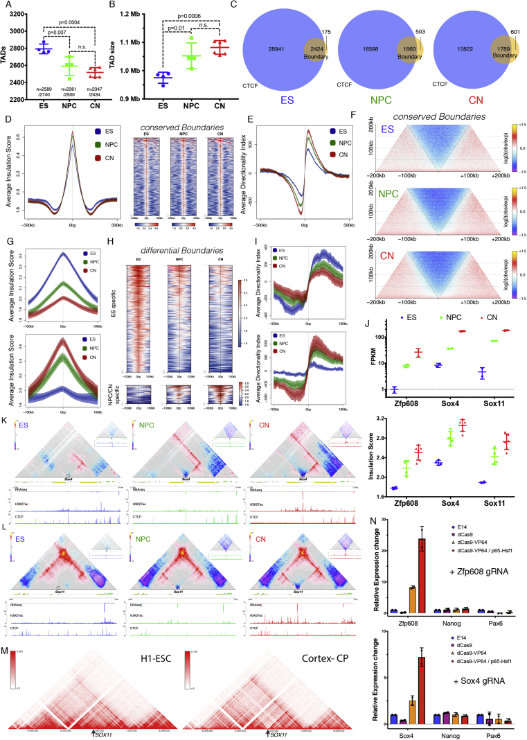
- TADs decrease in number and increase in size; CTCF-less boundaries increase. Developmentally regulated boundaries include 259 ES-specific and 54 neural-specific boundaries. CRISPR-dCas9 activation at Zfp608 and Sox4 caused >10- to 20-fold gene activation but no significant insulation or contact-map change, indicating transcription is correlated with but not sufficient for de novo TAD boundary formation.
- CTCF-mediated loops between convergent CTCF sites increase during differentiation despite decreased CTCF binding; ES-specific CTCF contacts and insulation are lost in NPCs, validated by 3D DNA FISH at the Zfp42 locus.
- Active promoters show CTCF-independent insulation and interact with other active promoters across TAD boundaries; gene bodies of exon-rich, highly expressed genes form long-range contacts in cis and trans, correlating with exon number/splicing. Polycomb-mediated contacts are disrupted during differentiation and correlate with Ring1B rather than H3K27me3. In vivo, neural TFs Pax6, NeuroD2, and Tbr1 organize cell-type-specific contacts, and enhancer-promoter contacts are mostly cell-type specific and generally established concomitantly with gene expression.
Methods
- In situ Hi-C was performed on FACS-purified G0/G1 mouse ES cells, NPCs, and CNs from an in vitro differentiation system, plus NPCs and CNs purified from E14.5 mouse neocortex in vivo. The study reports >40 billion paired-end reads and >17 billion uniquely mapped contacts, with >11 billion uniquely aligned contacts in vitro and ~3 billion per in vivo cell type; maximum resolution reached 750 bp.
- Complementary assays included RNA-seq, ChIP-seq for chromatin marks and factors such as CTCF and Ring1B, 3D DNA FISH, and CRISPR-dCas9-mediated gene activation.
- Hi-C analysis used fragment-end resolution, expected models generated with the Shaman R package, insulation scores, eigenvector-based A/B compartment assignment, aggregate Hi-C maps, and contact enrichment quantification.
Limitations
- The paper states that the in vitro system recapitulates some but not all aspects of cortical development, such as neuronal migration and morphogen signaling; it also notes that whether the observed gene-body contacts are directly linked to co-transcriptional splicing remains to be seen, and whether TF contacts represent true homotypic interactions is unresolved.
- The paper states that clear violations of a simple enhancer-promoter looping model exist, as some enhancer-promoter loops are pre-established.
- Evident from the text: Hi-C is population-averaged and cannot resolve single-cell or allele-specific heterogeneity; FISH validates only selected loci; dCas9 activation was tested at two loci; and in vitro versus in vivo differences may limit generalization.
Model-written summary. Check it against the paper before relying on it.
Integrity signals
Registry
Cites
Statistics
Figures
Verification
Claims the paper makes
90 Own result · 21 Not checked yet · 19 Own interpretation · 11 Own method · 5 No basis given · 1 Partly supported · accuracy not yet measured
A result the paper reports from its own data — it cites no other source for it, so there is none to check. The quote shows it is in the paper.
In the paper
“We found that transcription is correlated with chromatin insulation and long-range interactions, but dCas9-mediated activation is insufficient for creating TAD boundaries de novo.”
- Also stated in: § Transcription Is Correlated with but Not Sufficient to Induce Insulation at TAD Boundaries De Novo · hedged
“Therefore, transcriptional activation per se appears insufficient to cause chromatin insulation and create a TAD boundary.”
§ Multiscale 3D Genome Rewiring during Mouse Neural Development > Abstract
plain- Asserted: passes — The authors put it forward as true.
- Checkable: passes — It can be checked against evidence.
- Load-bearing: passes — The paper’s conclusions depend on it.
- Based: passes — The paper gives a reason why it holds.
- Also stated in: § Transcription Is Correlated with but Not Sufficient to Induce Insulation at TAD Boundaries De Novo · hedged
A result the paper reports from its own data — it cites no other source for it, so there is none to check. The quote shows it is in the paper.
In the paper
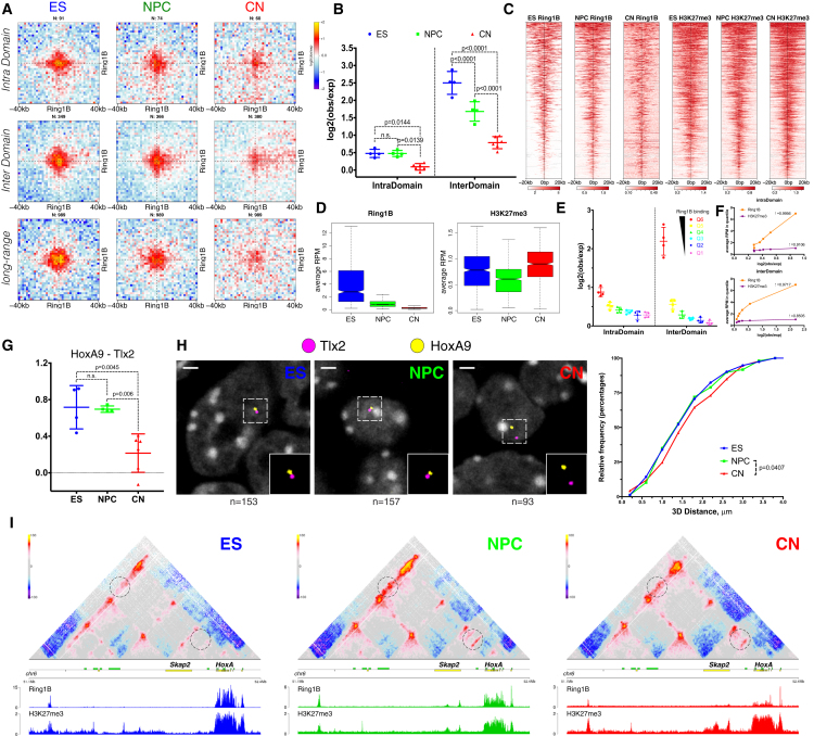
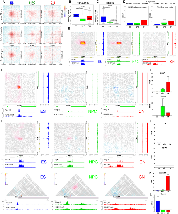
“An extensive Polycomb network in stem cells is disrupted, while dynamic interactions between neural transcription factors appear in vivo.”
- Also stated in: § Polycomb-Mediated Interactions Are Disrupted Independently of H3K27me3 during Neural Differentiation · boosted
“we observed a strong decrease in contact intensity between common H3K27me3 sites, which was especially notable at long distances (Figure S6A).”
§ Multiscale 3D Genome Rewiring during Mouse Neural Development > Abstract
boosteddirect- Asserted: passes — The authors put it forward as true.
- Checkable: passes — It can be checked against evidence.
- Load-bearing: passes — The paper’s conclusions depend on it.
- Based: passes — The paper gives a reason why it holds.
- Also stated in: § Polycomb-Mediated Interactions Are Disrupted Independently of H3K27me3 during Neural Differentiation · boosted
A result the paper reports from its own data — it cites no other source for it, so there is none to check. The quote shows it is in the paper.
In the paper
“Finally, cell type-specific enhancer-promoter contacts are established concomitant to gene expression.”
§ Multiscale 3D Genome Rewiring during Mouse Neural Development > Abstract
plaincorrelational- Asserted: passes — The authors put it forward as true.
- Checkable: passes — It can be checked against evidence.
- Load-bearing: passes — The paper’s conclusions depend on it.
- Based: passes — The paper gives a reason why it holds.
A result the paper reports from its own data — it cites no other source for it, so there is none to check. The quote shows it is in the paper.
In the paper
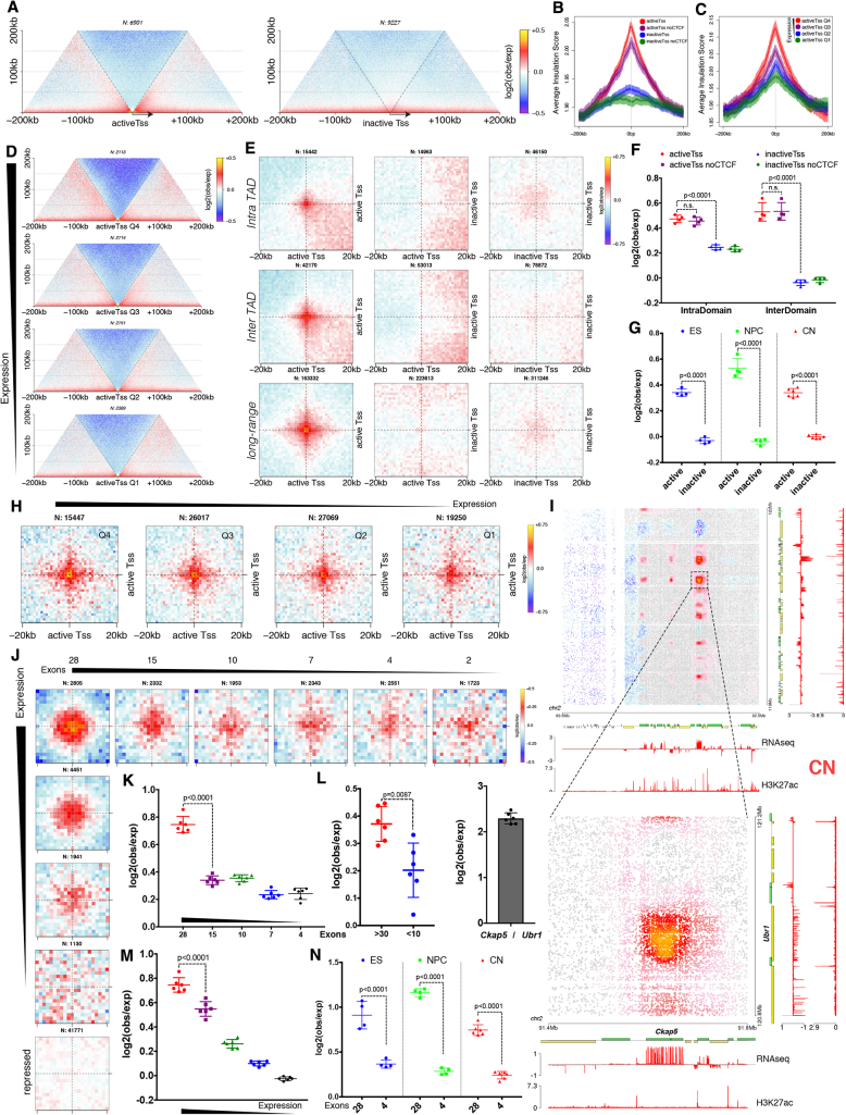
“Additionally, we discovered long-range contacts between gene bodies of exon-rich, active genes in all cell types.”
- Also stated in: § Active Gene Promoters and the Bodies of Exon-Rich Genes Interact at Multiple Genomic Scales · plain
“Finally, actively transcribed genes with a large number of exons engage in long-range chromatin loops in clusters both in cis- and in trans.”
§ Multiscale 3D Genome Rewiring during Mouse Neural Development > Abstract
plaincorrelational- Asserted: passes — The authors put it forward as true.
- Checkable: passes — It can be checked against evidence.
- Load-bearing: passes — The paper’s conclusions depend on it.
- Based: passes — The paper gives a reason why it holds.
- Also stated in: § Active Gene Promoters and the Bodies of Exon-Rich Genes Interact at Multiple Genomic Scales · plain
A result the paper reports from its own data — it cites no other source for it, so there is none to check. The quote shows it is in the paper.
In the paper
“We found that transcription is correlated with chromatin insulation and long-range interactions, but dCas9-mediated activation is insufficient for creating TAD boundaries de novo.”
§ Multiscale 3D Genome Rewiring during Mouse Neural Development > Abstract
plaincorrelational- Asserted: passes — The authors put it forward as true.
- Checkable: passes — It can be checked against evidence.
- Load-bearing: passes — The paper’s conclusions depend on it.
- Based: passes — The paper gives a reason why it holds.
A result the paper reports from its own data — it cites no other source for it, so there is none to check. The quote shows it is in the paper.
In the paper
“An extensive Polycomb network in stem cells is disrupted, while dynamic interactions between neural transcription factors appear in vivo.”
§ Multiscale 3D Genome Rewiring during Mouse Neural Development > Abstract
hedged- Asserted: passes — The authors put it forward as true.
- Checkable: passes — It can be checked against evidence.
- Load-bearing: passes — The paper’s conclusions depend on it.
- Based: passes — The paper gives a reason why it holds.
A result the paper reports from its own data — it cites no other source for it, so there is none to check. The quote shows it is in the paper.
In the paper
“We found that genes located in close proximity to the neural-specific TAD boundaries tend to be upregulated (Figures 2Fi and 2Gi)”
§ Multiscale 3D Genome Rewiring during Mouse Neural Development > Results > Transcription Is Correlated with but Not Sufficient to Induce Insulation at TAD Boundaries De Novo
plaincorrelational- Asserted: passes — The authors put it forward as true.
- Checkable: passes — It can be checked against evidence.
- Load-bearing: unclear — It is unclear whether the paper’s conclusions depend on it.
- Based: passes — The paper gives a reason why it holds.
- Rests on an assumption: The mechanisms contributing to developmentally regulated TAD borders remain poorly understood.
None of the sources cited for this claim have been checked yet.
In the paper
“we observed a similar increase in insulation around SOX11 (Figure S3M).”
§ Multiscale 3D Genome Rewiring during Mouse Neural Development > Results > Transcription Is Correlated with but Not Sufficient to Induce Insulation at TAD Boundaries De Novo
What the sources say
plaincorrelational- Asserted: passes — The authors put it forward as true.
- Checkable: passes — It can be checked against evidence.
- Load-bearing: passes — The paper’s conclusions depend on it.
- Based: passes — The paper gives a reason why it holds.
- Rests on an assumption: The mechanisms contributing to developmentally regulated TAD borders remain poorly understood.
A result the paper reports from its own data — it cites no other source for it, so there is none to check. The quote shows it is in the paper.
In the paper
“Highly conserved boundaries in our system were characterized by a small but consistent increase in insulation during differentiation (Figures S3D–S3F).”
§ Multiscale 3D Genome Rewiring during Mouse Neural Development > Results > Transcription Is Correlated with but Not Sufficient to Induce Insulation at TAD Boundaries De Novo
plaindirect- Asserted: passes — The authors put it forward as true.
- Checkable: passes — It can be checked against evidence.
- Load-bearing: unclear — It is unclear whether the paper’s conclusions depend on it.
- Based: passes — The paper gives a reason why it holds.
- Rests on an assumption: The mechanisms contributing to developmentally regulated TAD borders remain poorly understood.
A result the paper reports from its own data — it cites no other source for it, so there is none to check. The quote shows it is in the paper.
In the paper
“Analysis of TAD boundaries revealed that the proportion of the CTCF-less borders increased during differentiation (Figure S3C).”
§ Multiscale 3D Genome Rewiring during Mouse Neural Development > Results > Transcription Is Correlated with but Not Sufficient to Induce Insulation at TAD Boundaries De Novo
plaindirect- Asserted: passes — The authors put it forward as true.
- Checkable: passes — It can be checked against evidence.
- Load-bearing: passes — The paper’s conclusions depend on it.
- Based: passes — The paper gives a reason why it holds.
- Probably not a substantial claim. 14
- It may state two separate claims as one. 53
- The quote only partly states this claim. 1
The cited sources support only part of this claim — read each source’s verdict below.
In the paper
“At intermediate scales (100 kb to 1 Mb), a major discovery is the existence of topologically associating domains (TADs) (Dixon et al., 2012, Nora et al., 2012, Sexton et al., 2012).”
§ Multiscale 3D Genome Rewiring during Mouse Neural Development > Introduction
What the sources say
- Supportedcites Dixon et al., 2012 source
The Abstract identifies topological domains as a pervasive feature of mammalian genomes and reports 2,200 domains in mouse embryonic stem cells with a median size of 880 kb. That supports their existence at the intermediate scale described; the stated 100 kb–1 Mb is an approximate scale, not a range the paper assigns to every domain. (LLM, conf=0.87)
- Supportedcites Nora et al., 2012 source
The paper reports self-associating genomic blocks covering 0.2–1 Mb and identifies the resulting sub-megabase domains as TADs. That observed range falls within the citing sentence’s intermediate-scale band of 100 kb to 1 Mb; the paper does not claim to have observed a 100-kb TAD. (LLM, conf=0.90)
- Partly supportedcites Sexton et al., 2012 sourceExperimental — accuracy not yet measured
In “The Genome Is Partitioned into Well-Demarcated Physical Domains” (page unavailable), Sexton et al. identify 1,169 contact-enriched physical domains in the Drosophila genome, supporting the existence of TAD-like domains. The passages in our copy do not establish the specific 100 kb to 1 Mb size range attributed to this citation. (LLM, conf=0.82)
plain- Asserted: passes — The authors put it forward as true.
- Checkable: passes — It can be checked against evidence.
- Load-bearing: fails — The paper’s conclusions may not depend on it.
- Based: passes — The paper gives a reason why it holds.
Probably not a substantial claim. The paper’s conclusions may not depend on it.
- Supported
A result the paper reports from its own data — it cites no other source for it, so there is none to check. The quote shows it is in the paper.
In the paper
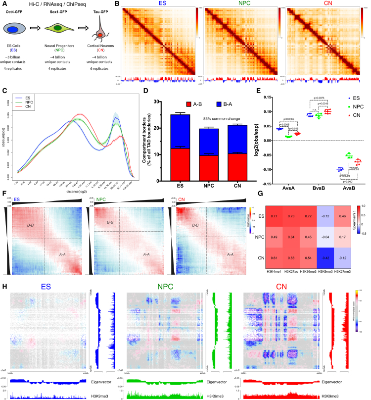
“During neural differentiation, contacts between active TADs become less pronounced while inactive TADs interact more strongly.”
- Also stated in: § Global Reorganization of the 3D Genome during Neural Differentiation · plain
“Surprisingly, the interaction strength between A-type domains decreased, whereas contacts within the B compartment became stronger between NPCs and CNs (Figures 1E and S1L).”
§ Multiscale 3D Genome Rewiring during Mouse Neural Development > Abstract
plaindirect- Asserted: passes — The authors put it forward as true.
- Checkable: passes — It can be checked against evidence.
- Load-bearing: passes — The paper’s conclusions depend on it.
- Based: passes — The paper gives a reason why it holds.
It may state two separate claims as one.
- Also stated in: § Global Reorganization of the 3D Genome during Neural Differentiation · plain
A result the paper reports from its own data — it cites no other source for it, so there is none to check. The quote shows it is in the paper.
In the paper
“In total, we sequenced over 40 billion paired-end reads that resulted in more than 17 billion uniquely mapped contacts.”
§ Multiscale 3D Genome Rewiring during Mouse Neural Development > Introduction
plain- Asserted: passes — The authors put it forward as true.
- Checkable: passes — It can be checked against evidence.
- Load-bearing: passes — The paper’s conclusions depend on it.
- Based: passes — The paper gives a reason why it holds.
It may state two separate claims as one.
A result the paper reports from its own data — it cites no other source for it, so there is none to check. The quote shows it is in the paper.
In the paper
“CTCF was bound to the Sox4 promoter already in ESs, yet insulation dramatically increased only when the gene became expressed at the NPC stage (Figures S3K and S3J).”
§ Multiscale 3D Genome Rewiring during Mouse Neural Development > Results > Transcription Is Correlated with but Not Sufficient to Induce Insulation at TAD Boundaries De Novo
plaincorrelationalSingle case- Asserted: passes — The authors put it forward as true.
- Checkable: passes — It can be checked against evidence.
- Load-bearing: passes — The paper’s conclusions depend on it.
- Based: passes — The paper gives a reason why it holds.
It may state two separate claims as one.
- Rests on an assumption: The mechanisms contributing to developmentally regulated TAD borders remain poorly understood.
A result the paper reports from its own data — it cites no other source for it, so there is none to check. The quote shows it is in the paper.
In the paper
“We then examined TADs and found that their number decreased during differentiation (Figure S3A), with a corresponding increase in size (Figure S3B).”
§ Multiscale 3D Genome Rewiring during Mouse Neural Development > Results > Transcription Is Correlated with but Not Sufficient to Induce Insulation at TAD Boundaries De Novo
plaincorrelational- Asserted: passes — The authors put it forward as true.
- Checkable: passes — It can be checked against evidence.
- Load-bearing: unclear — It is unclear whether the paper’s conclusions depend on it.
- Based: passes — The paper gives a reason why it holds.
It may state two separate claims as one.
A result the paper reports from its own data — it cites no other source for it, so there is none to check. The quote shows it is in the paper.
In the paper
“the correlation between signal enrichment and eigenvector value for active histone marks decreased during differentiation, while the anti-correlation between H3K9me3 and the eigenvector value became stronger”
§ Multiscale 3D Genome Rewiring during Mouse Neural Development > Results > Global Reorganization of the 3D Genome during Neural Differentiation
plaincorrelational- Asserted: passes — The authors put it forward as true.
- Checkable: passes — It can be checked against evidence.
- Load-bearing: unclear — It is unclear whether the paper’s conclusions depend on it.
- Based: passes — The paper gives a reason why it holds.
It may state two separate claims as one.
A result the paper reports from its own data — it cites no other source for it, so there is none to check. The quote shows it is in the paper.
In the paper
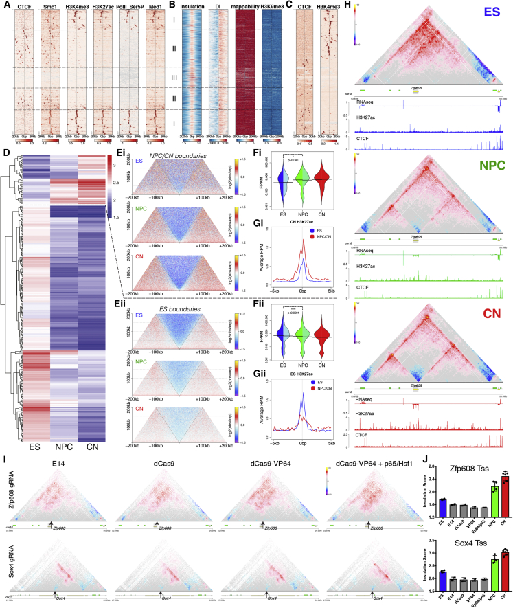
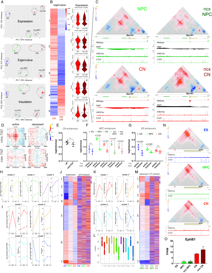
“a novel TAD boundary was formed at the transcriptional start site (Tss) of Zfp608 during differentiation (Figure 2H), concomitant with the activation of the gene (Figure S3J) but in the absence of CTCF binding.”
§ Multiscale 3D Genome Rewiring during Mouse Neural Development > Results > Transcription Is Correlated with but Not Sufficient to Induce Insulation at TAD Boundaries De Novo
plaincorrelationalSingle case- Asserted: passes — The authors put it forward as true.
- Checkable: passes — It can be checked against evidence.
- Load-bearing: passes — The paper’s conclusions depend on it.
- Based: passes — The paper gives a reason why it holds.
It may state two separate claims as one.
- Rests on an assumption: The mechanisms contributing to developmentally regulated TAD borders remain poorly understood.
A result the paper reports from its own data — it cites no other source for it, so there is none to check. The quote shows it is in the paper.
In the paper
“We observed three classes of boundaries: CTCF-positive boundaries, CTCF-negative boundaries close to active gene promoters, and a set of boundaries without enrichment of active marks (Figure 2A).”
§ Multiscale 3D Genome Rewiring during Mouse Neural Development > Results > Transcription Is Correlated with but Not Sufficient to Induce Insulation at TAD Boundaries De Novo
plain- Asserted: passes — The authors put it forward as true.
- Checkable: passes — It can be checked against evidence.
- Load-bearing: passes — The paper’s conclusions depend on it.
- Based: passes — The paper gives a reason why it holds.
It may state two separate claims as one.
A result the paper reports from its own data — it cites no other source for it, so there is none to check. The quote shows it is in the paper.
In the paper
“cohesin was found both at CTCF-positive boundaries, where it colocalized with CTCF, and on CTCF-negative borders marked by active transcription (Figure 2A).”
§ Multiscale 3D Genome Rewiring during Mouse Neural Development > Results > Transcription Is Correlated with but Not Sufficient to Induce Insulation at TAD Boundaries De Novo
plaincorrelational- Asserted: passes — The authors put it forward as true.
- Checkable: passes — It can be checked against evidence.
- Load-bearing: passes — The paper’s conclusions depend on it.
- Based: passes — The paper gives a reason why it holds.
It may state two separate claims as one.
A result the paper reports from its own data — it cites no other source for it, so there is none to check. The quote shows it is in the paper.
In the paper
“the absolute levels of Ring1B decreased during differentiation (with only a mild effect on gene expression [Figure S6D]), while H3K27me3 levels did not (Figure 5D).”
§ Multiscale 3D Genome Rewiring during Mouse Neural Development > Results > Polycomb-Mediated Interactions Are Disrupted Independently of H3K27me3 during Neural Differentiation
plain- Asserted: passes — The authors put it forward as true.
- Checkable: passes — It can be checked against evidence.
- Load-bearing: passes — The paper’s conclusions depend on it.
- Based: passes — The paper gives a reason why it holds.
It may state two separate claims as one.
A result the paper reports from its own data — it cites no other source for it, so there is none to check. The quote shows it is in the paper.
In the paper
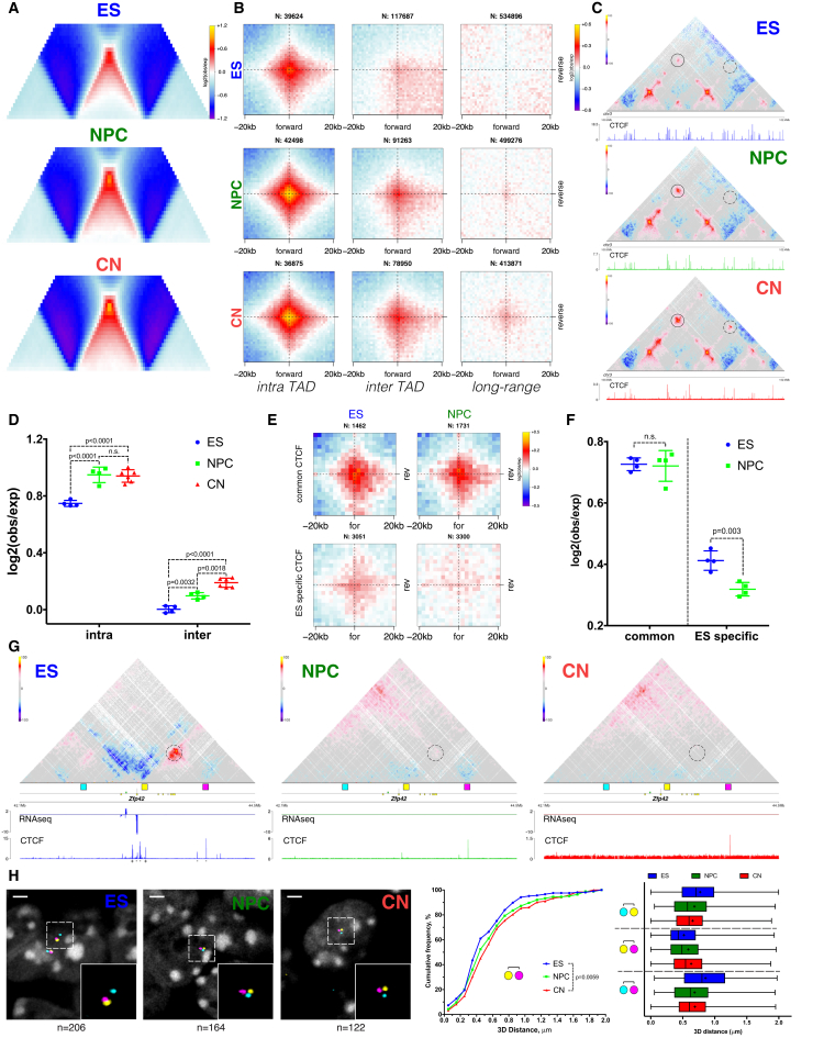
“In contrast, both the contact enrichment and the insulation between ES-specific CTCF regions were decreased in NPCs (Figures 3E, 3F and S4F).”
§ Multiscale 3D Genome Rewiring during Mouse Neural Development > Results > Dynamic CTCF-Based Loops and Insulation during Neural Differentiation
plain- Asserted: passes — The authors put it forward as true.
- Checkable: passes — It can be checked against evidence.
- Load-bearing: passes — The paper’s conclusions depend on it.
- Based: passes — The paper gives a reason why it holds.
It may state two separate claims as one.
None of the sources cited for this claim have been checked yet.
In the paper
“We observed strong enrichment as expected (Guo et al., 2015, Rao et al., 2014), and the loops were constrained primarily inside TADs and rarely crossed TAD boundaries (Figures 3B and 3D).”
§ Multiscale 3D Genome Rewiring during Mouse Neural Development > Results > Dynamic CTCF-Based Loops and Insulation during Neural Differentiation
What the sources say
boostedcorrelational- Asserted: passes — The authors put it forward as true.
- Checkable: passes — It can be checked against evidence.
- Load-bearing: passes — The paper’s conclusions depend on it.
- Based: passes — The paper gives a reason why it holds.
It may state two separate claims as one.
A result the paper reports from its own data — it cites no other source for it, so there is none to check. The quote shows it is in the paper.
In the paper
“Conserved CTCF were characterized by strong interactions in the convergent orientation (Figures 3E and 3F) and by strong insulation both in ESs and NPCs (Figure S4E).”
§ Multiscale 3D Genome Rewiring during Mouse Neural Development > Results > Dynamic CTCF-Based Loops and Insulation during Neural Differentiation
plaincorrelational- Asserted: passes — The authors put it forward as true.
- Checkable: passes — It can be checked against evidence.
- Load-bearing: passes — The paper’s conclusions depend on it.
- Based: passes — The paper gives a reason why it holds.
It may state two separate claims as one.
A result the paper reports from its own data — it cites no other source for it, so there is none to check. The quote shows it is in the paper.
In the paper
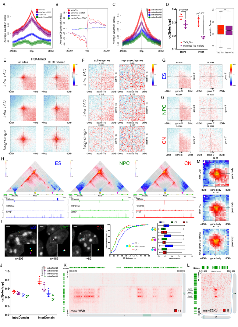
“we also identified clusters of very long-range (> 30 Mb) chromatin contacts between bodies of expressed genes in cis (Figures 4I and S5K) and also in trans (Figure S5L).”
§ Multiscale 3D Genome Rewiring during Mouse Neural Development > Results > Active Gene Promoters and the Bodies of Exon-Rich Genes Interact at Multiple Genomic Scales
plaincorrelational- Asserted: passes — The authors put it forward as true.
- Checkable: passes — It can be checked against evidence.
- Load-bearing: passes — The paper’s conclusions depend on it.
- Based: passes — The paper gives a reason why it holds.
It may state two separate claims as one.
A result the paper reports from its own data — it cites no other source for it, so there is none to check. The quote shows it is in the paper.
In the paper
“most of these interactions were not mediated by CTCF (Figure 4F) and were readily identified in all three cell types (Figure 4G).”
§ Multiscale 3D Genome Rewiring during Mouse Neural Development > Results > Active Gene Promoters and the Bodies of Exon-Rich Genes Interact at Multiple Genomic Scales
plain- Asserted: passes — The authors put it forward as true.
- Checkable: passes — It can be checked against evidence.
- Load-bearing: passes — The paper’s conclusions depend on it.
- Based: passes — The paper gives a reason why it holds.
It may state two separate claims as one.
A result the paper reports from its own data — it cites no other source for it, so there is none to check. The quote shows it is in the paper.
In the paper
“only the 3D FISH distance between the pair of probes containing the forward and the reverse CTCF site increased during differentiation, while the other probe pairs displayed the opposite effect (Figures 3H, S4H, and S4I).”
§ Multiscale 3D Genome Rewiring during Mouse Neural Development > Results > Dynamic CTCF-Based Loops and Insulation during Neural Differentiation
plaindirect- Asserted: passes — The authors put it forward as true.
- Checkable: passes — It can be checked against evidence.
- Load-bearing: passes — The paper’s conclusions depend on it.
- Based: passes — The paper gives a reason why it holds.
It may state two separate claims as one.
A result the paper reports from its own data — it cites no other source for it, so there is none to check. The quote shows it is in the paper.
In the paper
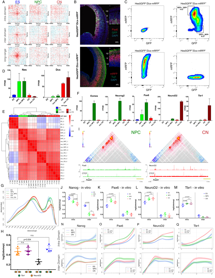
“the contact enrichment between gene bodies was highly correlated not only with expression levels, but also with the number of exons per gene (Figures 4J, 4K, and 4M), and was evident across a large range of genomic distances (Figure S5M) in all three cell types (Figure 4N).”
§ Multiscale 3D Genome Rewiring during Mouse Neural Development > Results > Active Gene Promoters and the Bodies of Exon-Rich Genes Interact at Multiple Genomic Scales
plaincorrelational- Asserted: passes — The authors put it forward as true.
- Checkable: passes — It can be checked against evidence.
- Load-bearing: passes — The paper’s conclusions depend on it.
- Based: passes — The paper gives a reason why it holds.
It may state two separate claims as one.
A result the paper reports from its own data — it cites no other source for it, so there is none to check. The quote shows it is in the paper.
In the paper
“However, the overall enrichment of CTCF-mediated contacts increased with neural differentiation, and even inter-domain contacts became apparent (Figures 3B–3D and S4B).”
§ Multiscale 3D Genome Rewiring during Mouse Neural Development > Results > Dynamic CTCF-Based Loops and Insulation during Neural Differentiation
plaincorrelational- Asserted: passes — The authors put it forward as true.
- Checkable: passes — It can be checked against evidence.
- Load-bearing: passes — The paper’s conclusions depend on it.
- Based: passes — The paper gives a reason why it holds.
It may state two separate claims as one.
A result the paper reports from its own data — it cites no other source for it, so there is none to check. The quote shows it is in the paper.
In the paper
“During differentiation, only the forward CTCF site became inaccessible to CTCF, and the chromatin loop disappeared (Figure 3G).”
§ Multiscale 3D Genome Rewiring during Mouse Neural Development > Results > Dynamic CTCF-Based Loops and Insulation during Neural Differentiation
plaindirectSingle case- Asserted: passes — The authors put it forward as true.
- Checkable: passes — It can be checked against evidence.
- Load-bearing: passes — The paper’s conclusions depend on it.
- Based: passes — The paper gives a reason why it holds.
It may state two separate claims as one.
In the paper
“general TFs such as Taf3 (Liu et al., 2011) appear to enhance interaction between promoters but had little effect on insulation (Figure S5D).”
§ Multiscale 3D Genome Rewiring during Mouse Neural Development > Results > Active Gene Promoters and the Bodies of Exon-Rich Genes Interact at Multiple Genomic Scales
What the sources say
- Not checked yetcites Liu et al., 2011 source
hedgedconditional- Asserted: passes — The authors put it forward as true.
- Checkable: passes — It can be checked against evidence.
- Load-bearing: unclear — It is unclear whether the paper’s conclusions depend on it.
- Based: passes — The paper gives a reason why it holds.
It may state two separate claims as one.
A result the paper reports from its own data — it cites no other source for it, so there is none to check. The quote shows it is in the paper.
In the paper
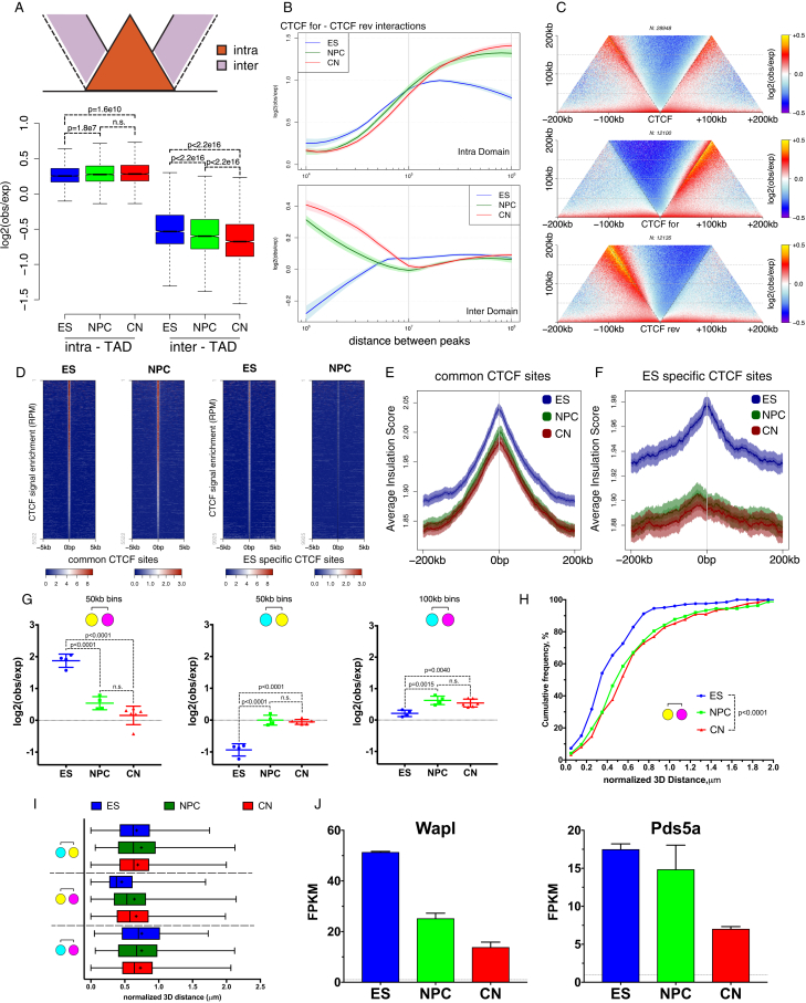
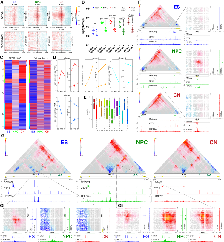
“we identified a strong preference for insulation centered on active Tss, but not on inactive ones, a phenomenon that was not dependent on CTCF binding (Figures 4A, 4B, S5A, and S5B).”
§ Multiscale 3D Genome Rewiring during Mouse Neural Development > Results > Active Gene Promoters and the Bodies of Exon-Rich Genes Interact at Multiple Genomic Scales
boostedcorrelational- Asserted: passes — The authors put it forward as true.
- Checkable: passes — It can be checked against evidence.
- Load-bearing: passes — The paper’s conclusions depend on it.
- Based: passes — The paper gives a reason why it holds.
It may state two separate claims as one.
A result the paper reports from its own data — it cites no other source for it, so there is none to check. The quote shows it is in the paper.
In the paper
“We observed that average intra-TAD contacts become stronger, while inter-TAD contacts appear to be depleted during differentiation (Figures 3A and S4A).”
§ Multiscale 3D Genome Rewiring during Mouse Neural Development > Results > Dynamic CTCF-Based Loops and Insulation during Neural Differentiation
hedgedcorrelational- Asserted: passes — The authors put it forward as true.
- Checkable: passes — It can be checked against evidence.
- Load-bearing: passes — The paper’s conclusions depend on it.
- Based: passes — The paper gives a reason why it holds.
It may state two separate claims as one.
A result the paper reports from its own data — it cites no other source for it, so there is none to check. The quote shows it is in the paper.
In the paper
“we observed no central enrichment when we performed the same analysis using instead 3′ gene ends (Figure S5F), showing that these interactions were specific to promoters and were correlated with the level of expression (Figures 4H and S5J).”
§ Multiscale 3D Genome Rewiring during Mouse Neural Development > Results > Active Gene Promoters and the Bodies of Exon-Rich Genes Interact at Multiple Genomic Scales
plaincorrelational- Asserted: passes — The authors put it forward as true.
- Checkable: passes — It can be checked against evidence.
- Load-bearing: passes — The paper’s conclusions depend on it.
- Based: passes — The paper gives a reason why it holds.
It may state two separate claims as one.
A result the paper reports from its own data — it cites no other source for it, so there is none to check. The quote shows it is in the paper.
In the paper
“active chromatin loops span across domains and can be observed even at long distances (Figure 4E), in contrast with CTCF-mediated contacts.”
§ Multiscale 3D Genome Rewiring during Mouse Neural Development > Results > Active Gene Promoters and the Bodies of Exon-Rich Genes Interact at Multiple Genomic Scales
plaincorrelational- Asserted: passes — The authors put it forward as true.
- Checkable: passes — It can be checked against evidence.
- Load-bearing: passes — The paper’s conclusions depend on it.
- Based: passes — The paper gives a reason why it holds.
It may state two separate claims as one.
In the paper
“Therefore, although we confirmed that most TAD boundaries are conserved (Dixon et al., 2012), novel borders can occur at promoters of developmentally regulated genes.”
§ Multiscale 3D Genome Rewiring during Mouse Neural Development > Discussion
What the sources say
- Not checked yetcites Dixon et al., 2012 source
plain- Asserted: passes — The authors put it forward as true.
- Checkable: passes — It can be checked against evidence.
- Load-bearing: fails — The paper’s conclusions may not depend on it.
- Based: passes — The paper gives a reason why it holds.
Probably not a substantial claim. The paper’s conclusions may not depend on it.
A result the paper reports from its own data — it cites no other source for it, so there is none to check. The quote shows it is in the paper.
In the paper
“Moreover, we identified regions that switch compartments between the in vitro and the in vivo systems, which were accompanied with corresponding changes in gene expression (Figures S8B and S8C).”
§ Multiscale 3D Genome Rewiring during Mouse Neural Development > Results > Cell-Type Specific Chromatin Folding Is Organized around the Neural Transcription Factors Pax6, NeuroD2, and Tbr1 In Vivo
plaincorrelational- Asserted: passes — The authors put it forward as true.
- Checkable: passes — It can be checked against evidence.
- Load-bearing: passes — The paper’s conclusions depend on it.
- Based: passes — The paper gives a reason why it holds.
It may state two separate claims as one.
A result the paper reports from its own data — it cites no other source for it, so there is none to check. The quote shows it is in the paper.
In the paper
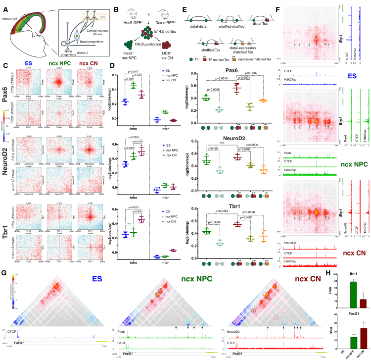
“We observed a strong decrease in the interactions between Sox2 promoter and the ES-specific enhancer (Figure 7G, blue arrow) during differentiation, which coincides with a decrease in both CTCF binding and the H3K27ac mark on the enhancer (Figure 7Gi).”
§ Multiscale 3D Genome Rewiring during Mouse Neural Development > Results > Enhancer-Promoter Contacts Are Mostly Cell-Type Specific and Are Generally Established Concomitantly with Gene Expression
boostedcorrelational- Asserted: passes — The authors put it forward as true.
- Checkable: passes — It can be checked against evidence.
- Load-bearing: passes — The paper’s conclusions depend on it.
- Based: passes — The paper gives a reason why it holds.
It may state two separate claims as one.
A result the paper reports from its own data — it cites no other source for it, so there is none to check. The quote shows it is in the paper.
In the paper
“NeuroD2 and Tbr1 interactions were also mostly constrained inside TADs (Figures 6C, 6D, S7P, and S7Q) but increased during differentiation and were the strongest in CNs in vivo.”
§ Multiscale 3D Genome Rewiring during Mouse Neural Development > Results > Cell-Type Specific Chromatin Folding Is Organized around the Neural Transcription Factors Pax6, NeuroD2, and Tbr1 In Vivo
plaindirect- Asserted: passes — The authors put it forward as true.
- Checkable: passes — It can be checked against evidence.
- Load-bearing: passes — The paper’s conclusions depend on it.
- Based: passes — The paper gives a reason why it holds.
It may state two separate claims as one.
A result the paper reports from its own data — it cites no other source for it, so there is none to check. The quote shows it is in the paper.
In the paper
“These interactions are strongly correlated with the number of splicing events per gene with the strongest contacts occurring between genes that undergo most splicing.”
§ Multiscale 3D Genome Rewiring during Mouse Neural Development > Discussion
boostedcorrelational- Asserted: passes — The authors put it forward as true.
- Checkable: passes — It can be checked against evidence.
- Load-bearing: passes — The paper’s conclusions depend on it.
- Based: passes — The paper gives a reason why it holds.
It may state two separate claims as one.
A result the paper reports from its own data — it cites no other source for it, so there is none to check. The quote shows it is in the paper.
In the paper
“The analysis of a well-controlled differentiation system and its in vivo cell counterparts shows that cell differentiation is accompanied by a global chromatin reorganization and a change in compartmentalization with a decrease in long-range interactions between A-type domains concomitant with an increase in contacts between inactive B-type domains.”
§ Multiscale 3D Genome Rewiring during Mouse Neural Development > Discussion
plaincorrelational- Asserted: passes — The authors put it forward as true.
- Checkable: passes — It can be checked against evidence.
- Load-bearing: passes — The paper’s conclusions depend on it.
- Based: passes — The paper gives a reason why it holds.
It may state two separate claims as one.
The paper states this without a source or data behind it here, so there is nothing to check it against. The quote shows it is in the paper.
In the paper
“In ESs, the strong long-range interactions also involve Polycomb-bound genes and, to a lesser extent, genes bound by pluripotency TFs.”
§ Multiscale 3D Genome Rewiring during Mouse Neural Development > Discussion
plaincorrelational- Asserted: passes — The authors put it forward as true.
- Checkable: passes — It can be checked against evidence.
- Load-bearing: unclear — It is unclear whether the paper’s conclusions depend on it.
- Based: passes — The paper gives a reason why it holds.
It may state two separate claims as one.
A result the paper reports from its own data — it cites no other source for it, so there is none to check. The quote shows it is in the paper.
In the paper
“These networks are reorganized in neuronal differentiation, which in the case of Polycomb appears to correlate with PRC1 binding levels.”
§ Multiscale 3D Genome Rewiring during Mouse Neural Development > Discussion
hedgedcorrelational- Asserted: passes — The authors put it forward as true.
- Checkable: passes — It can be checked against evidence.
- Load-bearing: passes — The paper’s conclusions depend on it.
- Based: passes — The paper gives a reason why it holds.
It may state two separate claims as one.
A result the paper reports from its own data — it cites no other source for it, so there is none to check. The quote shows it is in the paper.
In the paper
“We identified a NPC-specific enhancer, which interacted strongly with the promoter of the neuronal TF Brn2 gene only in NPCs, and this interaction was disrupted in CNs when the enhancer was inactive (Figure 7F).”
§ Multiscale 3D Genome Rewiring during Mouse Neural Development > Results > Enhancer-Promoter Contacts Are Mostly Cell-Type Specific and Are Generally Established Concomitantly with Gene Expression
boosteddirect- Asserted: passes — The authors put it forward as true.
- Checkable: passes — It can be checked against evidence.
- Load-bearing: passes — The paper’s conclusions depend on it.
- Based: passes — The paper gives a reason why it holds.
It may state two separate claims as one.
A result the paper reports from its own data — it cites no other source for it, so there is none to check. The quote shows it is in the paper.
In the paper
“Principal component analysis (PCA) also confirmed that NPC populations, either in vitro or in vivo, are highly similar to each other and are distinct from CNs and vice versa (Figure S8A).”
§ Multiscale 3D Genome Rewiring during Mouse Neural Development > Results > Cell-Type Specific Chromatin Folding Is Organized around the Neural Transcription Factors Pax6, NeuroD2, and Tbr1 In Vivo
plain- Asserted: passes — The authors put it forward as true.
- Checkable: passes — It can be checked against evidence.
- Load-bearing: passes — The paper’s conclusions depend on it.
- Based: passes — The paper gives a reason why it holds.
It may state two separate claims as one.
A result the paper reports from its own data — it cites no other source for it, so there is none to check. The quote shows it is in the paper.
In the paper
“Furthermore, the average Hi-C scores and the correlation between expression and chromatin contacts were strongly decreased when we randomly shuffled the position of the enhancer region within the same TAD (Figures 7D, 7E, and S8H).”
§ Multiscale 3D Genome Rewiring during Mouse Neural Development > Results > Enhancer-Promoter Contacts Are Mostly Cell-Type Specific and Are Generally Established Concomitantly with Gene Expression
boosteddirect- Asserted: passes — The authors put it forward as true.
- Checkable: passes — It can be checked against evidence.
- Load-bearing: passes — The paper’s conclusions depend on it.
- Based: passes — The paper gives a reason why it holds.
It may state two separate claims as one.
A result the paper reports from its own data — it cites no other source for it, so there is none to check. The quote shows it is in the paper.
In the paper
“We observed a cell-type specific contact enrichment between Pax6-bound sites strongest in ncx NPC where Pax6 is highly expressed (Figures 6C and 6D).”
§ Multiscale 3D Genome Rewiring during Mouse Neural Development > Results > Cell-Type Specific Chromatin Folding Is Organized around the Neural Transcription Factors Pax6, NeuroD2, and Tbr1 In Vivo
plaincorrelational- Asserted: passes — The authors put it forward as true.
- Checkable: passes — It can be checked against evidence.
- Load-bearing: passes — The paper’s conclusions depend on it.
- Based: passes — The paper gives a reason why it holds.
It may state two separate claims as one.
A result the paper reports from its own data — it cites no other source for it, so there is none to check. The quote shows it is in the paper.
In the paper
“Although we did identify instances of pre-set chromatin interactions between enhancers and their cognate target genes that precede transcriptional activation (Figures 7C, S8N, and S8O), the majority of those interactions appear to be established concomitantly to gene expression and are also disrupted when the genes become repressed.”
§ Multiscale 3D Genome Rewiring during Mouse Neural Development > Results > Enhancer-Promoter Contacts Are Mostly Cell-Type Specific and Are Generally Established Concomitantly with Gene Expression
hedgedcorrelational- Asserted: passes — The authors put it forward as true.
- Checkable: passes — It can be checked against evidence.
- Load-bearing: passes — The paper’s conclusions depend on it.
- Based: passes — The paper gives a reason why it holds.
It may state two separate claims as one.
A result the paper reports from its own data — it cites no other source for it, so there is none to check. The quote shows it is in the paper.
In the paper
“mean nuclear radius of the ES, NPC and CNs population were calculated (ES = 1.73 ± 0.28; NPC = 1.39 ± 0.24; CN = 1.43 ± 0.20).”
§ Multiscale 3D Genome Rewiring during Mouse Neural Development > STAR★Methods > Quantification and Statistical Analysis
plain- Asserted: passes — The authors put it forward as true.
- Checkable: passes — It can be checked against evidence.
- Load-bearing: passes — The paper’s conclusions depend on it.
- Based: passes — The paper gives a reason why it holds.
It may state two separate claims as one.
A result the paper reports from its own data — it cites no other source for it, so there is none to check. The quote shows it is in the paper.
In the paper
“Domains in each cluster exhibit distinct signature based on the enrichment of chromatin marks, replication timing and Lamin B1 DamID enrichment where available (Figure S1I), prompting us to assign cluster 1 to the B-, inactive compartment and cluster 2 to the A-, active compartment.”
§ Multiscale 3D Genome Rewiring during Mouse Neural Development > STAR★Methods > Quantification and Statistical Analysis
plaindirect- Asserted: passes — The authors put it forward as true.
- Checkable: passes — It can be checked against evidence.
- Load-bearing: passes — The paper’s conclusions depend on it.
- Based: passes — The paper gives a reason why it holds.
It may state two separate claims as one.
What the paper did — it cites no source for this, so there is none to check. The quote shows it is in the paper.
In the paper
“We comprehensively mapped 3D chromatin organization during mouse neural differentiation in vitro and in vivo, generating the highest-resolution Hi-C maps available to date.”
- Also stated in: § Global Reorganization of the 3D Genome during Neural Differentiation · plain
“We reached a maximum resolution of 750 bp—the highest to date (Figure S1F).”
§ Multiscale 3D Genome Rewiring during Mouse Neural Development > Abstract
plain- Asserted: passes — The authors put it forward as true.
- Checkable: passes — It can be checked against evidence.
- Load-bearing: passes — The paper’s conclusions depend on it.
- Based: passes — The paper gives a reason why it holds.
It may state two separate claims as one.
- Rests on an assumption: Our understanding of the interaction dynamics at the smallest scales during developmental processes is currently limited.
- Rests on an assumption: The relation between loop extrusion models and transcription remains unclear.
- Also stated in: § Global Reorganization of the 3D Genome during Neural Differentiation · plain
A conclusion the paper draws from its own results — it cites no other source for it, so there is none to check. The quote shows it is in the paper.
In the paper
“Our data demonstrate that cellular differentiation involves changes at all scales of folding, and in addition to CTCF-dependent processes, it includes major changes in Polycomb and in transcription factor (TF) interaction networks.”
§ Multiscale 3D Genome Rewiring during Mouse Neural Development > Introduction
boosteddirect- Asserted: passes — The authors put it forward as true.
- Checkable: passes — It can be checked against evidence.
- Load-bearing: passes — The paper’s conclusions depend on it.
- Based: passes — The paper gives a reason why it holds.
It may state two separate claims as one.
- Rests on an assumption: Our understanding of the interaction dynamics at the smallest scales during developmental processes is currently limited.
- Rests on an assumption: The relation between loop extrusion models and transcription remains unclear.
In the paper
“At larger scales, interactions between domains are thought to give rise to two main types of spatial compartments referred to as “A” and “B” (Lieberman-Aiden et al., 2009)”
§ Multiscale 3D Genome Rewiring during Mouse Neural Development > Introduction
What the sources say
- Not checked yetcites Lieberman-Aiden et al., 2009 source
hedgeddirect- Asserted: passes — The authors put it forward as true.
- Checkable: passes — It can be checked against evidence.
- Load-bearing: fails — The paper’s conclusions may not depend on it.
- Based: passes — The paper gives a reason why it holds.
Probably not a substantial claim. The paper’s conclusions may not depend on it.
What the paper did — it cites no source for this, so there is none to check. The quote shows it is in the paper.
In the paper
“verified that these borders represent a genuine loss or gain of insulation, respectively, using aggregate Hi-C maps (Figure 2E), insulation score (Figures S3G and S3H), and directionality index (DI) (Figure S3I).”
§ Multiscale 3D Genome Rewiring during Mouse Neural Development > Results > Transcription Is Correlated with but Not Sufficient to Induce Insulation at TAD Boundaries De Novo
boosted- Asserted: passes — The authors put it forward as true.
- Checkable: passes — It can be checked against evidence.
- Load-bearing: passes — The paper’s conclusions depend on it.
- Based: passes — The paper gives a reason why it holds.
It may state two separate claims as one.
- Rests on an assumption: The mechanisms contributing to developmentally regulated TAD borders remain poorly understood.
In the paper
“recent evidence indicates that domains and compartment formation can be at least partially uncoupled and may result from different biological phenomena (Nora et al., 2017).”
§ Multiscale 3D Genome Rewiring during Mouse Neural Development > Introduction
What the sources say
- Not checked yetcites Nora et al., 2017 source
hedgedconditional- Asserted: passes — The authors put it forward as true.
- Checkable: passes — It can be checked against evidence.
- Load-bearing: fails — The paper’s conclusions may not depend on it.
- Based: passes — The paper gives a reason why it holds.
Probably not a substantial claim. The paper’s conclusions may not depend on it. It may state two separate claims as one.
None of the sources cited for this claim have been checked yet.
In the paper
“Domain insulation has been shown to be important for gene expression and physiology (Flavahan et al., 2016, Lupiáñez et al., 2015).”
§ Multiscale 3D Genome Rewiring during Mouse Neural Development > Introduction
What the sources say
boosteddirect- Asserted: passes — The authors put it forward as true.
- Checkable: passes — It can be checked against evidence.
- Load-bearing: fails — The paper’s conclusions may not depend on it.
- Based: passes — The paper gives a reason why it holds.
Probably not a substantial claim. The paper’s conclusions may not depend on it.
In the paper
“which are functionally related to gene expression and can switch extensively during differentiation (Dixon et al., 2015).”
§ Multiscale 3D Genome Rewiring during Mouse Neural Development > Introduction
What the sources say
- Not checked yetcites Dixon et al., 2015 source
plaincorrelational- Asserted: passes — The authors put it forward as true.
- Checkable: passes — It can be checked against evidence.
- Load-bearing: fails — The paper’s conclusions may not depend on it.
- Based: passes — The paper gives a reason why it holds.
Probably not a substantial claim. The paper’s conclusions may not depend on it. It may state two separate claims as one.
In the paper
“very few studies using mostly in vitro cultured cells have achieved high resolution (Rao et al., 2014).”
§ Multiscale 3D Genome Rewiring during Mouse Neural Development > Introduction
What the sources say
- Not checked yetcites Rao et al., 2014 source
plain- Asserted: passes — The authors put it forward as true.
- Checkable: passes — It can be checked against evidence.
- Load-bearing: passes — The paper’s conclusions depend on it.
- Based: passes — The paper gives a reason why it holds.
Probably not a substantial claim.
What the paper did — it cites no source for this, so there is none to check. The quote shows it is in the paper.
In the paper
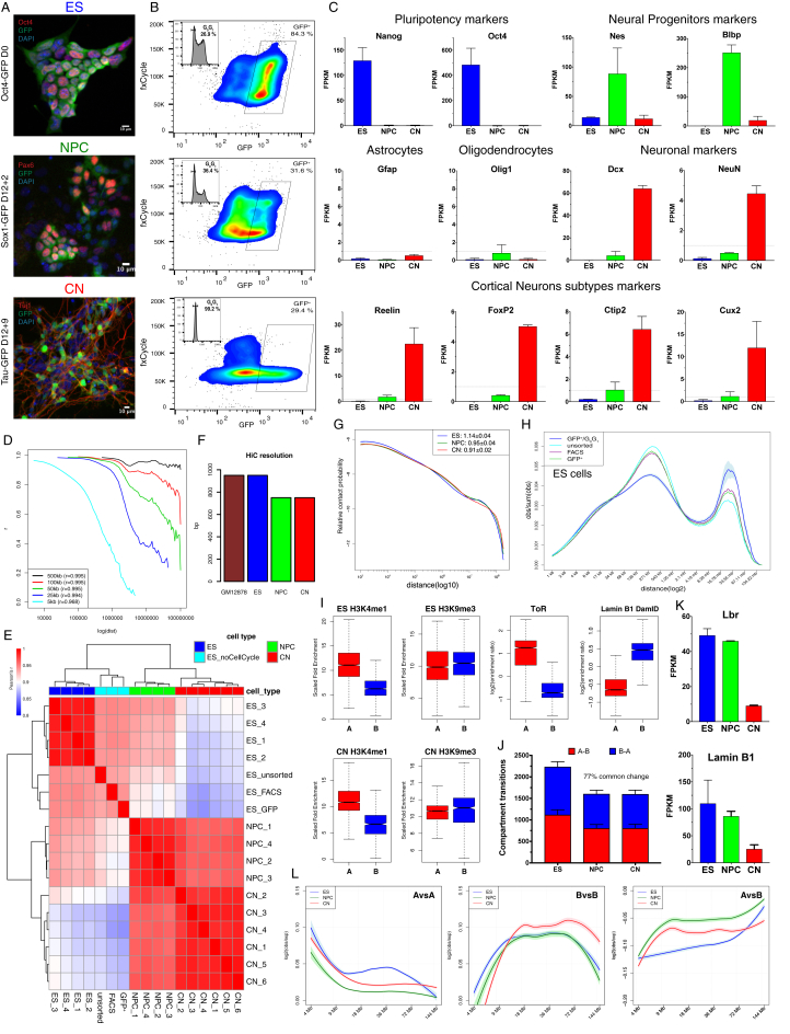
“we employed a fluorescence-activated cell sorting (FACS) approach, which allowed us to purify G0G1 cells based on DNA content”
§ Multiscale 3D Genome Rewiring during Mouse Neural Development > Results > Global Reorganization of the 3D Genome during Neural Differentiation
plaindirect- Asserted: passes — The authors put it forward as true.
- Checkable: passes — It can be checked against evidence.
- Load-bearing: fails — The paper’s conclusions may not depend on it.
- Based: passes — The paper gives a reason why it holds.
Probably not a substantial claim. The paper’s conclusions may not depend on it.
What the paper did — it cites no source for this, so there is none to check. The quote shows it is in the paper.
In the paper
“we controlled for cell type heterogeneity and cell-cycle variation.”
- Also stated in: § Global Reorganization of the 3D Genome during Neural Differentiation · plain
“we employed a fluorescence-activated cell sorting (FACS) approach, which allowed us to purify G0G1 cells based on DNA content”
§ Multiscale 3D Genome Rewiring during Mouse Neural Development > Introduction
plain- Asserted: passes — The authors put it forward as true.
- Checkable: passes — It can be checked against evidence.
- Load-bearing: passes — The paper’s conclusions depend on it.
- Based: passes — The paper gives a reason why it holds.
It may state two separate claims as one.
- Also stated in: § Global Reorganization of the 3D Genome during Neural Differentiation · plain
None of the sources cited for this claim have been checked yet.
In the paper
“It is known that architectural proteins such as CTCF and cohesin play a role (Haarhuis et al., 2017, Nora et al., 2017, Phillips-Cremins et al., 2013)”
§ Multiscale 3D Genome Rewiring during Mouse Neural Development > Introduction
What the sources say
boostedcorrelational- Asserted: passes — The authors put it forward as true.
- Checkable: passes — It can be checked against evidence.
- Load-bearing: fails — The paper’s conclusions may not depend on it.
- Based: passes — The paper gives a reason why it holds.
Probably not a substantial claim. The paper’s conclusions may not depend on it.
What the paper did — it cites no source for this, so there is none to check. The quote shows it is in the paper.
In the paper
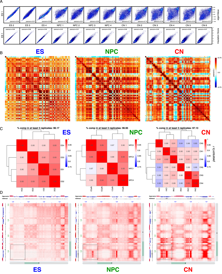
“Biological replicates were highly correlated at all resolutions (Figure S1D) and for each different cell type (Figures S1E and S2A).”
§ Multiscale 3D Genome Rewiring during Mouse Neural Development > Results > Global Reorganization of the 3D Genome during Neural Differentiation
plaincorrelational- Asserted: passes — The authors put it forward as true.
- Checkable: passes — It can be checked against evidence.
- Load-bearing: passes — The paper’s conclusions depend on it.
- Based: passes — The paper gives a reason why it holds.
It may state two separate claims as one.
A conclusion the paper draws from its own results — it cites no other source for it, so there is none to check. The quote shows it is in the paper.
In the paper
“In conclusion, a major genome-folding reprogramming occurs during neural differentiation with a progressive increase in compartment size, decreased interactions within the A compartment, and a concomitant increase in interactions between B-type domains.”
§ Multiscale 3D Genome Rewiring during Mouse Neural Development > Results > Global Reorganization of the 3D Genome during Neural Differentiation
plaindirect- Asserted: passes — The authors put it forward as true.
- Checkable: passes — It can be checked against evidence.
- Load-bearing: passes — The paper’s conclusions depend on it.
- Based: passes — The paper gives a reason why it holds.
It may state two separate claims as one.
- Rests on an assumption: Our understanding of the interaction dynamics at the smallest scales during developmental processes is currently limited.
- Rests on an assumption: The relation between loop extrusion models and transcription remains unclear.
None of the sources cited for this claim have been checked yet.
In the paper
“The deposition of chromatin marks is thought to contribute to this process (Dixon et al., 2015, Nora et al., 2012)”
§ Multiscale 3D Genome Rewiring during Mouse Neural Development > Introduction
What the sources say
hedgedconditional- Asserted: passes — The authors put it forward as true.
- Checkable: passes — It can be checked against evidence.
- Load-bearing: fails — The paper’s conclusions may not depend on it.
- Based: passes — The paper gives a reason why it holds.
Probably not a substantial claim. The paper’s conclusions may not depend on it.
A conclusion the paper draws from its own results — it cites no other source for it, so there is none to check. The quote shows it is in the paper.
In the paper
“In summary, promoters of active genes are characterized by strong insulation, which is correlated with transcriptional activity, but is mostly CTCF independent.”
§ Multiscale 3D Genome Rewiring during Mouse Neural Development > Results > Active Gene Promoters and the Bodies of Exon-Rich Genes Interact at Multiple Genomic Scales
plaincorrelational- Asserted: passes — The authors put it forward as true.
- Checkable: passes — It can be checked against evidence.
- Load-bearing: passes — The paper’s conclusions depend on it.
- Based: passes — The paper gives a reason why it holds.
It may state two separate claims as one.
None of the sources cited for this claim have been checked yet.
In the paper
“Polycomb-mediated interactions have been previously reported in mouse ESs using a Capture-C approach (Schoenfelder et al., 2015b) and are a prominent feature in Drosophila (Bantignies et al., 2011).”
§ Multiscale 3D Genome Rewiring during Mouse Neural Development > Results > Polycomb-Mediated Interactions Are Disrupted Independently of H3K27me3 during Neural Differentiation
What the sources say
- Not checked yetcites Schoenfelder et al., 2015b
- Not checked yetcites Bantignies et al., 2011 source
plain- Asserted: passes — The authors put it forward as true.
- Checkable: passes — It can be checked against evidence.
- Load-bearing: fails — The paper’s conclusions may not depend on it.
- Based: passes — The paper gives a reason why it holds.
Probably not a substantial claim. The paper’s conclusions may not depend on it. It may state two separate claims as one.
A conclusion the paper draws from its own results — it cites no other source for it, so there is none to check. The quote shows it is in the paper.
In the paper
“Active Tss maintain contacts with the gene body and, contrary to CTCF interactions, can interact with other transcribed Tss across TAD boundaries.”
§ Multiscale 3D Genome Rewiring during Mouse Neural Development > Results > Active Gene Promoters and the Bodies of Exon-Rich Genes Interact at Multiple Genomic Scales
plaincorrelational- Asserted: passes — The authors put it forward as true.
- Checkable: passes — It can be checked against evidence.
- Load-bearing: passes — The paper’s conclusions depend on it.
- Based: passes — The paper gives a reason why it holds.
It may state two separate claims as one.
In the paper
“As many as 40–50% of the CTCF sites may change in different cell types (Chen et al., 2012).”
§ Multiscale 3D Genome Rewiring during Mouse Neural Development > Results > Dynamic CTCF-Based Loops and Insulation during Neural Differentiation
What the sources say
- Not checked yetcites Chen et al., 2012 source
hedgedconditional- Asserted: passes — The authors put it forward as true.
- Checkable: passes — It can be checked against evidence.
- Load-bearing: fails — The paper’s conclusions may not depend on it.
- Based: passes — The paper gives a reason why it holds.
Probably not a substantial claim. The paper’s conclusions may not depend on it.
None of the sources cited for this claim have been checked yet.
In the paper
“Chromatin insulation occurs at multiple levels and leads to a hierarchical 3D nuclear organization, whereby smaller, less insulated regions (called also sub-TADs [Flavahan et al., 2016, Phillips-Cremins et al., 2013] or contact domains [Rao et al., 2014]) are nested inside TADs, which are usually bigger and more strongly insulated (Dixon et al., 2012, Nora et al., 2012, Sexton et al., 2012).”
§ Multiscale 3D Genome Rewiring during Mouse Neural Development > Results > Dynamic CTCF-Based Loops and Insulation during Neural Differentiation
What the sources say
plaindirect- Asserted: passes — The authors put it forward as true.
- Checkable: passes — It can be checked against evidence.
- Load-bearing: passes — The paper’s conclusions depend on it.
- Based: passes — The paper gives a reason why it holds.
It may state two separate claims as one.
None of the sources cited for this claim have been checked yet.
In the paper
“However, very few public chromatin immunoprecipitation sequencing (ChIP-seq) profiles exist, and most of those have been performed in the developing mouse neocortex (Bayam et al., 2015, Notwell et al., 2016, Sun et al., 2015).”
§ Multiscale 3D Genome Rewiring during Mouse Neural Development > Results > Cell-Type Specific Chromatin Folding Is Organized around the Neural Transcription Factors Pax6, NeuroD2, and Tbr1 In Vivo
What the sources say
plain- Asserted: passes — The authors put it forward as true.
- Checkable: passes — It can be checked against evidence.
- Load-bearing: passes — The paper’s conclusions depend on it.
- Based: passes — The paper gives a reason why it holds.
It may state two separate claims as one.
What the paper did — it cites no source for this, so there is none to check. The quote shows it is in the paper.
In the paper
“We performed RNA-seq and verified our approach using known markers for neural progenitors (Nestin) and differentiating neurons (Dcx) (Figure S7D).”
§ Multiscale 3D Genome Rewiring during Mouse Neural Development > Results > Cell-Type Specific Chromatin Folding Is Organized around the Neural Transcription Factors Pax6, NeuroD2, and Tbr1 In Vivo
plain- Asserted: passes — The authors put it forward as true.
- Checkable: passes — It can be checked against evidence.
- Load-bearing: passes — The paper’s conclusions depend on it.
- Based: passes — The paper gives a reason why it holds.
The quote only partly states this claim.
What the paper did — it cites no source for this, so there is none to check. The quote shows it is in the paper.
In the paper
“Pearson correlation coefficient (Figure S7E), comparison of the eigenvector values, insulation score, and contact probability (Figures S7G and S8A) confirmed the high quality of the data and that, importantly, samples group together based on cell type.”
§ Multiscale 3D Genome Rewiring during Mouse Neural Development > Results > Cell-Type Specific Chromatin Folding Is Organized around the Neural Transcription Factors Pax6, NeuroD2, and Tbr1 In Vivo
boostedcorrelational- Asserted: passes — The authors put it forward as true.
- Checkable: passes — It can be checked against evidence.
- Load-bearing: passes — The paper’s conclusions depend on it.
- Based: passes — The paper gives a reason why it holds.
It may state two separate claims as one.
In the paper
“Pax6 is one of the few “master regulator” neural TFs with a well-known role in cortical development (Manuel et al., 2015).”
§ Multiscale 3D Genome Rewiring during Mouse Neural Development > Results > Cell-Type Specific Chromatin Folding Is Organized around the Neural Transcription Factors Pax6, NeuroD2, and Tbr1 In Vivo
What the sources say
- Not checked yetcites Manuel et al., 2015 source
boosted- Asserted: passes — The authors put it forward as true.
- Checkable: passes — It can be checked against evidence.
- Load-bearing: fails — The paper’s conclusions may not depend on it.
- Based: passes — The paper gives a reason why it holds.
Probably not a substantial claim. The paper’s conclusions may not depend on it.
A conclusion the paper draws from its own results — it cites no other source for it, so there is none to check. The quote shows it is in the paper.
In the paper
“These results suggest that E-P interactions are highly dynamic and cell-type specific.”
§ Multiscale 3D Genome Rewiring during Mouse Neural Development > Results > Enhancer-Promoter Contacts Are Mostly Cell-Type Specific and Are Generally Established Concomitantly with Gene Expression
hedgedcorrelational- Asserted: passes — The authors put it forward as true.
- Checkable: passes — It can be checked against evidence.
- Load-bearing: passes — The paper’s conclusions depend on it.
- Based: passes — The paper gives a reason why it holds.
It may state two separate claims as one.
A conclusion the paper draws from its own results — it cites no other source for it, so there is none to check. The quote shows it is in the paper.
In the paper
“Finally, E-P interactions are highly dynamic and are usually established concomitantly with gene expression.”
§ Multiscale 3D Genome Rewiring during Mouse Neural Development > Discussion
plaincorrelational- Asserted: passes — The authors put it forward as true.
- Checkable: passes — It can be checked against evidence.
- Load-bearing: passes — The paper’s conclusions depend on it.
- Based: passes — The paper gives a reason why it holds.
It may state two separate claims as one.
What the paper did — it cites no source for this, so there is none to check. The quote shows it is in the paper.
In the paper
“Boundaries within 10Kb of each other were merged and only boundaries, which were detected in at least 3 biological replicates, were retained.”
§ Multiscale 3D Genome Rewiring during Mouse Neural Development > STAR★Methods > Quantification and Statistical Analysis
plain- Asserted: passes — The authors put it forward as true.
- Checkable: passes — It can be checked against evidence.
- Load-bearing: passes — The paper’s conclusions depend on it.
- Based: passes — The paper gives a reason why it holds.
Probably not a substantial claim.
The paper relies on this without support.
Our understanding of the interaction dynamics at the smallest scales during developmental processes is currently limited.
“However, our understanding of the interaction dynamics at the smallest scales during developmental processes is currently limited.”
The paper relies on this without support.
The relation between loop extrusion models and transcription remains unclear.
“However, the relation between such models and transcription remains unclear.”
The paper relies on this without support.
The mechanisms contributing to developmentally regulated TAD borders remain poorly understood.
“yet the mechanisms contributing to developmentally regulated borders remain poorly understood.”
The paper relies on this without support.
The majority of strong Polycomb-bound regions are on gene promoters.
“As the majority of strong Polycomb-bound regions are on gene promoters, we examined whether their interaction might depend on paused Pol II that is located at bivalent gene promoters (Min et al., 2011).”
The paper relies on this without support.
Enhancer-promoter contacts have been difficult to observe in Hi-C, and their strength relative to surrounding regions is unclear.
“Enhancer-promoter (E-P) contacts have been difficult to observe in Hi-C, and it is unclear how strong they are compared to the surrounding regions.”
The paper relies on this without support.
The in vitro differentiation system recapitulates some aspects of cortical development but not others such as neuronal migration and morphogen signaling.
“Furthermore, although the in vitro system we employed recapitulates some aspects of cortical development, other features, such as neuronal migration and morphogen signaling, are not.”
The paper relies on this without support.
The vast majority of ultra-close cis Hi-C contacts (separated by less than 1 kb) originate from non-digested DNA.
“Contacts separated by less than 1kb were not considered for subsequent analysis, as the vast majority of this ultra-close cis contacts originate from non-digested DNA.”
Claims other papers make about this one
Each is checked against this paper’s own text: does it say what the citing paper says it does?
The source backs part of the claim, not all of it — or backs it for a different population, condition or comparison.
In the citing paper
“The Sox2 gene has an essential enhancer, the Sox2 Control Region (SCR), which was found by 3C-derived techniques to loop to the Sox2 promoter (for example, [379, 401]).”
From Transcriptional enhancers and their communication with gene promoters (2021) · cites this paper as [401]
Experimental — accuracy not yet measuredThe source backs part of the claim, not all of it — or backs it for a different population, condition or comparison.
In the citing paper
“active promoters and enhancers can likely give rise to TAD boundaries even in the absence of convergent CTCF sites [401].”
From Transcriptional enhancers and their communication with gene promoters (2021) · cites this paper as [401]
Experimental — accuracy not yet measuredThe cited source says what the claim attributes to it.
In the citing paper
“Interestingly, Hi-C data obtained using differentiated mouse neurons led us to detect chromatin interactions between HAR202 and the Npas3 promoter (Bonev et al. 2017; supplementary fig. S8, Supplementary Material online).”
From The Human Accelerated Region HAR202 Controls NPAS3 Expression in the Developing Forebrain Displaying Differential Enhancer Activity Between Modern and Archaic Human Sequences (2024) · cites this paper as Bonev et al. 2017
The cited source says what the claim attributes to it.
In the citing paper
“The majority of specific enhancer–promoter loops follow this pattern and are highly enriched within, compared with across, TAD boundaries [277, 401, 405].”
From Transcriptional enhancers and their communication with gene promoters (2021) · cites this paper as [401]
In the citing paper
“The 3D genome plays an important role in neuronal gene expression and function”
From Neuronal DNA double-strand breaks lead to genome structural variations and 3D genome disruption in neurodegeneration (2023) · cites this paper as [96]
In the citing paper
“5C maps from our mature primary cortical neurons were highly correlated with and exhibited similar loops as published Hi-C maps from ES cell-derived cortical neurons”
From Three-dimensional genome restructuring across timescales of activity-induced neuronal gene expression (2020) · cites this paper as [33]
In the citing paper
“We applied published methods17 to identify 24,937 loops in cortical neurons”
From Three-dimensional genome restructuring across timescales of activity-induced neuronal gene expression (2020) · cites this paper as [33]
Self-check
Percentages, sums and reported differences re-computed from the paper’s own numbers.
Each contradiction between two passages listed here was confirmed by an independent check.
Rated minor: it would not touch a result — a value no result rests on, a p-value that stays on the same side of the significance level, or a conflict that is clerical, resolved elsewhere in the paper, or outside its own findings.
In the paper
§ Multiscale 3D Genome Rewiring during Mouse Neural Development > Results > Transcription Is Correlated with but Not Sufficient to Induce Insulation at TAD Boundaries De Novo
“We used the CRISPR-dCas9 system (Konermann et al., 2015) to activate gene expression at the endogenous Zfp608 and Sox4 loci”
§ Multiscale 3D Genome Rewiring during Mouse Neural Development > STAR★Methods > Experimental Model and Subject Details
“Guide RNAs (Zfp604 – AGAAAGCGGAATGAGAAGTT and Sox4 - TTGCTCTGTAAATTGGAATG) were designed and cloned”
Rated minor: it would not touch a result — a value no result rests on, a p-value that stays on the same side of the significance level, or a conflict that is clerical, resolved elsewhere in the paper, or outside its own findings.
In the paper
§ Multiscale 3D Genome Rewiring during Mouse Neural Development > STAR★Methods > Key Resources Table
“| Strand specific total RNA from sorted Hes5-GFP-/Dcx-mRFP+ ncx_NPC cells | This study | GEO: GSE96107 |”
§ Multiscale 3D Genome Rewiring during Mouse Neural Development > Results > Cell-Type Specific Chromatin Folding Is Organized around the Neural Transcription Factors Pax6, NeuroD2, and Tbr1 In Vivo
“GFP-/RFP+ (“ncx CN”) populations from the same embryonic brains”
Rated minor: it would not touch a result — a value no result rests on, a p-value that stays on the same side of the significance level, or a conflict that is clerical, resolved elsewhere in the paper, or outside its own findings.
In the paper
§ Multiscale 3D Genome Rewiring during Mouse Neural Development > STAR★Methods > Method Details
“The appropriate gates to isolate GFP+/RFP- and RFP-/GFP+ cells were set as described in Figure S7B.”
§ Multiscale 3D Genome Rewiring during Mouse Neural Development > Results > Cell-Type Specific Chromatin Folding Is Organized around the Neural Transcription Factors Pax6, NeuroD2, and Tbr1 In Vivo
“GFP+/RFP- (referred to as “ncx NPC” henceafter) and GFP-/RFP+ (“ncx CN”) populations from the same embryonic brains”
Rated minor: it would not touch a result — a value no result rests on, a p-value that stays on the same side of the significance level, or a conflict that is clerical, resolved elsewhere in the paper, or outside its own findings.
In the paper
§ Multiscale 3D Genome Rewiring during Mouse Neural Development > Results > Polycomb-Mediated Interactions Are Disrupted Independently of H3K27me3 during Neural Differentiation
“a loop was formed specifically in NPCs between the Cacna2d1 promoter and another NPC-specific Ring1B site located ∼500 kb downstream in the gene body (Figure S6J).”
§ Multiscale 3D Genome Rewiring during Mouse Neural Development > Results > Polycomb-Mediated Interactions Are Disrupted Independently of H3K27me3 during Neural Differentiation
“(J) HiC contact maps showing ∼150Kb region around Cacna2d1 promoter. Note the appearance of NPC-specific Ring1B/H3K27me3 site inside Cacna2d1 gene body, which coincides with an interaction between this region and the Cacna2d1 promoter.”
Citations
Cites
A 3D Map of the Human Genome at Kilobase Resolution Reveals Principles of Chromatin Looping
Rao, S. S. P., Huntley, M. H., Durand, N. C., Stamenova, E. K., Bochkov, I. D., Robinson, J. T., Sanborn, A. L., Machol, I., Omer, A. D., Lander, E. S., et al. (2014) · Cell · doi:10.1016/j.cell.2014.11.021 · Cited by 9,212
Comprehensive Mapping of Long-Range Interactions Reveals Folding Principles of the Human Genome
Lieberman-Aiden, E., van Berkum, N. L., Williams, L., Imakaev, M., Ragoczy, T., Telling, A., Amit, I., Lajoie, B. R., Sabo, P. J., Dorschner, M. O., et al. (2009) · Science · doi:10.1126/science.1181369 · Cited by 8,898
Topological domains in mammalian genomes identified by analysis of chromatin interactions
Dixon, J. R., Selvaraj, S., Yue, F., Kim, A., Li, Y., Shen, Y., Hu, M., Liu, J. S., & Ren, B. (2012) · Nature · doi:10.1038/nature11082 · Cited by 6,829
Spatial partitioning of the regulatory landscape of the X-inactivation centre
Nora, E. P., Lajoie, B. R., Schulz, E. G., Giorgetti, L., Okamoto, I., Servant, N., Piolot, T., van Berkum, N. L., Meisig, J., Sedat, J., et al. (2012) · Nature · doi:10.1038/nature11049 · Cited by 2,895
Genome-scale transcriptional activation by an engineered CRISPR-Cas9 complex
Konermann, S., Brigham, M. D., Trevino, A. E., Joung, J., Abudayyeh, O. O., Barcena, C., Hsu, P. D., Habib, N., Gootenberg, J. S., Nishimasu, H., et al. (2015) · Nature · doi:10.1038/nature14136 · Cited by 2,825
Disruptions of Topological Chromatin Domains Cause Pathogenic Rewiring of Gene-Enhancer Interactions
Lupiáñez, D. G., Kraft, K., Heinrich, V., Krawitz, P., Brancati, F., Klopocki, E., Horn, D., Kayserili, H., Opitz, J. M., Laxova, R., et al. (2015) · Cell · doi:10.1016/j.cell.2015.04.004 · Cited by 2,132
Formation of chromosomal domains by loop extrusion
Fudenberg, G., Imakaev, M., Lu, C., Goloborodko, A., Abdennur, N., & Mirny, L. A. (2016) · Cell Reports · doi:10.1016/j.celrep.2016.04.085 · Cited by 2,003
Three-dimensional folding and functional organization principles of the Drosophila genome
Sexton, T., Yaffe, E., Kenigsberg, E., Bantignies, F., Leblanc, B., Hoichman, M., Parrinello, H., Tanay, A., & Cavalli, G. (2012) · Cell · doi:10.1016/j.cell.2012.01.010 · Cited by 1,983
Self-citationMediator and cohesin connect gene expression and chromatin architecture
Kagey, M. H., Newman, J. J., Bilodeau, S., Zhan, Y., Orlando, D. A., van Berkum, N. L., Ebmeier, C. C., Goossens, J., Rahl, P. B., Levine, S. S., et al. (2010) · Nature · doi:10.1038/nature09380 · Cited by 1,939
Sanborn, A. L., Rao, S. S. P., Huang, S.-C., Durand, N. C., Huntley, M. H., Jewett, A. I., Bochkov, I. D., Chinnappan, D., Cutkosky, A., Li, J., et al. (2015) · Proceedings of the National Academy of Sciences · doi:10.1073/pnas.1518552112 · Cited by 1,730
Cited by
Sorted by citations
Items 901–999 of 999
A universal polymer signature in Hi-C resolves cohesin loop density and supports monomeric extrusion
Polovnikov, K., & Starkov, D. (2026) · Proceedings of the National Academy of Sciences · doi:10.1073/pnas.2534385123 · Cited by 3
Wei, X., Tran, D., & Diao, Y. (2023) · Current Protocols · doi:10.1002/cpz1.899 · Cited by 3
Fan, S., Dang, D., Gao, L., & Zhang, S. (2024) · Advanced Science · doi:10.1002/advs.202406364 · Cited by 4
Zhang, R., Sun, J., Liu, S., Ding, J., & Xiang, M. (2024) · Communications Biology · doi:10.1038/s42003-024-07230-1 · Cited by 3
Gene Doping Detection From the Perspective of 3D Genome
Ren, X., Shi, Y., Xiao, B., Su, X., Shi, H., He, G., Chen, P., Wu, D., & Shi, Y. Y. (2025) · Drug Testing and Analysis · doi:10.1002/dta.3850 · Cited by 3
Chromatin and epigenetic regulation in malignant tumors: A comprehensive review
Zhang, X., Liu, D., Chen, X., Li, T., & Wu, G. (2025) · Annals of the New York Academy of Sciences · doi:10.1111/nyas.70005 · Cited by 3
Liang, H., Berger, B., & Singh, R. (2026) · Cell Systems · doi:10.1016/j.cels.2026.101675 · Cited by 3
Disorder of three‐dimensional chromosome structure plays a role in carcinogenesis
Zhang, L., Liu, F., Wu, L., Fu, S., Xing, L., Zhang, L., Wang, X., & Wang, Y.-X. (2021) · Clinical and Translational Discovery · doi:10.1002/ctd2.17 · Cited by 3
Tran, J. R., Zheng, X., Adam, S. A., Goldman, R. D., & Zheng, Y. (2022) · Nucleic Acids Research · doi:10.1093/nar/gkac762 · Cited by 4
Nanoscale nuclear environments, fine-scale 3D genome organization and transcription regulation
Li, J., & Pertsinidis, A. (2022) · Current Opinion in Systems Biology · doi:10.1016/j.coisb.2022.100436 · Cited by 3
Davidson, C., Wordsworth, B. P., Cohen, C., Knight, J. C., & Vecellio, M. L. (2023) · Frontiers in Genetics · doi:10.3389/fgene.2023.1129207 · Cited by 2
CscoreTool-M infers 3D sub-compartment probabilities within cell population
Zheng, X., Tran, J. R., & Zheng, Y. (2023) · Bioinformatics · doi:10.1093/bioinformatics/btad314 · Cited by 3
“We then applied CscoreTool-M to mESC Hi-C data (Bonev et al. 2017), and calculated the correlation coefficients with NAD-seq and Lamin-B1 DamID (Fig.”
MethodPandupuspitasari, N. S., Khan, F. A., Huang, C., Ali, A., Yousaf, M. R., Shakeel, F., Putri, E. M., Negara, W., Muktiani, A., Prasetiyono, B. W. H. E., et al. (2023) · Functional & Integrative Genomics · doi:10.1007/s10142-023-01146-5 · Cited by 3
Zhang, S., Song, Y., Liu, M., Yuan, Z., Zhang, M., Zhang, H., Seim, I., Fan, G., Liu, S., & Liu, X. (2023) · DNA Research · doi:10.1093/dnares/dsad018 · Cited by 3
Emerging role of epigenetics in human neurodevelopmental disorders
Mastrototaro, G., Sessa, A., & Zaghi, M. (2023) · Elsevier eBooks · doi:10.1016/b978-0-443-18661-5.00022-1 · Cited by 3
Rojas, C. R., Cercy, J., Perillous, S., Gonthier‐Guéret, C., Montibus, B., Maupetit‐Mehouas, S., Espinadel, A., Dupré, M., Hong, C. C., Hata, K., et al. (2024) · Human Genetics and Genomics Advances · doi:10.1016/j.xhgg.2024.100271 · Cited by 3
Li, M., Yang, J., Xiao, R., Liu, Y., Hu, J., Li, T., Wu, P., Mei-li, Z., Huang, Y., Sun, Y., et al. (2024) · Cell Proliferation · doi:10.1111/cpr.13639 · Cited by 3
“The distributions of regional ICF values varied across WT and trisomic mESCs (Figure 3D), but were overall lower than that of mouse neural progenitor cells (NPCs) and CNs, 61 consistent with differentiated cells having increased chromosomal intermingling.”
Deciphering the dynamical chromosome structural reorganizations in human neural development
Chu, X., Feng, C., & Wang, J. (2024) · Physical Review Research · doi:10.1103/physrevresearch.6.023309 · Cited by 3
SRF promotes long-range chromatin loop formation and stem cell pluripotency
Tsaytler, P. A., Blaess, G., Scholze‐Wittler, M., Meierhofer, D., Wittler, L., Koch, F., & Herrmann, B. G. (2024) · Cell Reports · doi:10.1016/j.celrep.2024.114846 · Cited by 3
Sun, Y., Li, M., Ning, C., Gao, L., Liu, Z., Zhong, S., Lv, J., Ke, Y., Wang, X., Ma, Q., et al. (2025) · Cell Discovery · doi:10.1038/s41421-025-00798-w · Cited by 3
“Physical chromatin loops can bring distal cis elements to the target gene promoter in a proximal 3D space to regulate gene expression 8,16,24 – 26 .”
Plaisancié, J., Angée, C., Erjavec, E., Raymond‐Letron, I., Douet, J., Goetz, M., Vincent‐Delorme, C., Karemaker, I. D., Baltissen, M. P. A., Vermeulen, M., et al. (2025) · Investigative Ophthalmology & Visual Science · doi:10.1167/iovs.66.11.47 · Cited by 3
“For chromatin conformation analysis of the Foxe3 locus in mice, we used mouse embryonic stem cell (mESC) Hi-C data from Bonev et al., 20 generated from intact cell nuclei using restriction enzyme-mediated DNA cleavage prior to proximity-based ligation.”
Transcription of carbonyl reductase 1 is regulated by DNA topoisomerase II beta
Khazeem, M. M., Cowell, I. G., Harkin, L. F., Casement, J., & Austin, C. A. (2020) · FEBS Letters · doi:10.1002/1873-3468.13904 · Cited by 3
HiCmapTools: a tool to access HiC contact maps
Chang, J., Weng, Y.-F., Chang, W.-T., Lin, F.-A., & Cavalli, G. (2022) · BMC Bioinformatics · doi:10.1186/s12859-022-04589-y · Cited by 3
“Although a substantial proportion of TADs form loops, with loop bases frequently located at the TAD boundaries in mammals [17, 18], few examples of TAD loop structure have been reported in the fly genome [19].”
BackgroundSelf-citationHow chromosome topologies get their shape: views from proximity ligation and microscopy methods
Huang, Y., Neijts, R., & de Laat, W. L. (2020) · FEBS Letters · doi:10.1002/1873-3468.13961 · Cited by 3
“The SCR is located at ~ 100 kb downstream of the gene promoter [67,68] and, as indicated by 3C-based meth-ods, displays highly enriched contacts with the promoter region in Sox2 -expressing cells [28,42].”
Chromatin Structure from Development to Ageing
Ayala-Guerrero, L., Claudio-Galeana, S., Furlan-Magaril, M., & Castro‐Obregón, S. (2023) · Sub-cellular biochemistry/Subcellular biochemistry · doi:10.1007/978-3-031-21410-3_2 · Cited by 2
The Chromosome Conformation Capture (3C) in Drosophila melanogaster
Sardo, F. L. (2020) · Methods in molecular biology · doi:10.1007/978-1-0716-0664-3_2 · Cited by 3
Simultaneous production of diverse neuronal subtypes during early corticogenesisPreprint
Magrinelli, E., Wagener, R. J., & Jabaudon, D. (2018) · bioRxiv (Cold Spring Harbor Laboratory) · doi:10.1101/369678 · Cited by 3
Chandradoss, K. R., Guthikonda, P. K., Kethavath, S., Dass, M., Singh, H., Nayak, R., Kurukuti, S., & Sandhu, K. S. (2018) · bioRxiv (Cold Spring Harbor Laboratory) · doi:10.1101/498006 · Cited by 3
Coolpup.py – a versatile tool to perform pile-up analysis of Hi-C data
Flyamer, I. M., Illingworth, R. S., & Bickmore, W. A. (2019) · Figshare · doi:10.5281/zenodo.3246468 · Cited by 4
“py to publicly available Hi-C data [23,24] using distiller (https://github.”
MethodStefano, M. D., Stadhouders, R., Farabella, I., Castillo, D., Serra, F., Graf, T., & Martı́-Renom, M. A. (2019) · bioRxiv (Cold Spring Harbor Laboratory) · doi:10.1101/642009 · Cited by 3
Tian, G. G., Zhao, X., Xie, W., Li, X., Hou, C., Wang, Y., Wang, L., Zhao, X., Li, H., Li, J., et al. (2019) · bioRxiv (Cold Spring Harbor Laboratory) · doi:10.1101/787689 · Cited by 3
“Based on previous results, both A/B compartment status and TADs could affect gene expression 27,28 .”
Result3D genome evolution and reorganization in the Drosophila melanogaster species groupPreprint
Torosin, N. S., Anand, A., Golla, T. R., Cao, W., & Ellison, C. E. (2020) · bioRxiv (Cold Spring Harbor Laboratory) · doi:10.1101/2020.04.09.033753 · Cited by 3
The role of insulators and transcription in 3D chromatin organisation of fliesPreprint
Chathoth, K. T., Mikheeva, L. A., Crevel, G., Wolfe, J. C., Hunter, I., Beckett-Doyle, S., Cotterill, S., Dai, H., Harrison, A., & Zabet, N. R. (2021) · bioRxiv (Cold Spring Harbor Laboratory) · doi:10.1101/2021.04.26.441424 · Cited by 3
A novel enhancer that regulates Bdnf expression in developing neuronsPreprint
Brookes, E., Au, H. Y. A., Varsally, W., Barrington, C., Hadjur, S., & Riccio, A. (2021) · bioRxiv (Cold Spring Harbor Laboratory) · doi:10.1101/2021.11.18.469096 · Cited by 3
“Analysis of published high resolution HiC data from mouse embryonic stem cells (ESCs) differentiated into NPCs and cortical neurons (CNs) (Bonev et al., 2017) revealed a sub-TAD encompassing the Bdnf gene and a downstream gene-free region adjacent to the closest downstream gene, Lin7c…”
BackgroundInfluentialPollex, T., Rabinowitz, A. H., Gambetta, M. C., Marco-Ferreres, R., Viales, R. R., Jankowski, A., Schaub, C., & Furlong, E. E. M. (2022) · bioRxiv (Cold Spring Harbor Laboratory) · doi:10.1101/2022.12.07.519443 · Cited by 3
“This includes motifs for several transcription factors essential for the development of the respective tissues, including Mef2, enriched at the ‘other end‘ of Muscle (compared to Neuron) specific interactions at 10-12h, and Ttk and l(3)neo38 enriched at Neuronal (compared to Muscle) specific interactions at 10-12h.”
BackgroundMethodTranscription regulates the spatio-temporal dynamics of genes through micro-compartmentalizationPreprint
Salari, H., Fourel, G., & Jost, D. (2023) · bioRxiv (Cold Spring Harbor Laboratory) · doi:10.1101/2023.07.18.549489 · Cited by 3
Competition between transcription and loop extrusion modulates promoter and enhancer dynamicsPreprint
Sexton, T., Platania, A., Erb, C., Barbieri, M., Molcrette, B., Grandgirard, E., de Kort, M. A. C., Meaburn, K. J., Taylor, T., Shchuka, V. M., et al. (2023) · Research Square · doi:10.21203/rs.3.rs-3164817/v1 · Cited by 3
Synergistic insulation of regulatory domains by developmental genes and clusters of CTCF sitesPreprint
Ealo, T., Sánchez-Gaya, V., Respuela, P., Martín, M. M., Martín-Batista, E., Haro, E., & Rada-Iglesias, Á. (2023) · bioRxiv (Cold Spring Harbor Laboratory) · doi:10.1101/2023.12.15.571760 · Cited by 3
“Regarding mESC data, a bigwig file (file ID: 4DNFIMVJ2YV3) with mm10 insulation scores obtained from previously generated Hi-C data 72 was downloaded from the 4D Nucleome data portal 98 .”
BackgroundMethodHanafiah, A., Geng, Z., Liu, T., Tai, Y. T., Cai, W., Wang, Q., Christensen, N. D., Liu, Y., Yue, F., & Gao, Z. (2024) · bioRxiv (Cold Spring Harbor Laboratory) · doi:10.1101/2024.11.13.623456 · Cited by 3
Lee, U., Laguillo-Diego, A., Wong, W., Ni, Z., Cheng, L., Li, J., Pelham-Webb, B., Pertsinidis, A., Leslie, C., & Apostolou, E. (2025) · doi:10.1101/2025.02.13.638153 · Cited by 3
Hao, Y., Li, Z., Lara, E., Ramos, D. M., Santiana, M., Jin, B., Epstein, J., Camacho, J. J., Carmiol, N., Kowal, I., et al. (2025) · bioRxiv (Cold Spring Harbor Laboratory) · doi:10.1101/2025.03.25.645331 · Cited by 3
“Over the past decades, large-scale genomics and transcriptomic studies have provided quantitative insights into gene expression trajectories during neuronal development 13-15 .”
Promoter strength and position govern promoter competition via transcript-dependent insulationPreprint
Koska, M., Nagano, M., Swigut, T., Boettiger, A. N., Hansen, A. S., & Wysocka, J. (2025) · bioRxiv (Cold Spring Harbor Laboratory) · doi:10.1101/2025.05.06.652547 · Cited by 3
“Although the downstream landing pad is within the same TAD as Sox2 and SE 23 , it lies outside of the previously reported Sox2 -SE loop contact demarcated by the convergent CTCF sites 24,25 .”
Zagirova, D., Kononkova, A. D., Morozov, K. V., Molodova, M. N., Vaulin, N., Dudkovskaia, A., Dozorova, P. I., Efimova, O., Tvorogova, A. V., Ulianov, K. A., et al. (2026) · Genome Research · doi:10.1101/gr.281488.125 · Cited by 3
Nr2f1 enhancers have distinct functions in controlling Nr2f1 expression during cortical development
Liu, Z., Ypsilanti, A. R., Markenscoff-Papadimitriou, E., Dickel, D. E., Sanders, S., Dong, S., Pennacchio, L. A., Visel, A., & Rubenstein, J. L. R. (2024) · Proceedings of the National Academy of Sciences · doi:10.1073/pnas.2402368121 · Cited by 2
“As Nr2f1 regulates cortical patterning (31, 34), and as Nr2f1 expression is reduced at E12.”
Nucleosome organization of mouse embryos during pre-implantation development
Zeng, J., Tu, X., Qu, S., Chen, X., Wang, Y., Liu, X., Kang, E., Tian, Y., Xiang, Q., Lai, B., et al. (2025) · Scientific Reports · doi:10.1038/s41598-025-05642-5 · Cited by 2
“CTCF.ES-Bruce4(43,085 peaks) 20 , GSM2533853(121406 peaks) 22 , GSM3771259(52,089 peaks) 23 .”
Bai, X., Tang, X., Wang, Y., Yue, S., Xu, X., Hu, P., Xu, J., Li, Y., Wang, J., Tao, H., et al. (2025) · BMC Biology · doi:10.1186/s12915-025-02259-y · Cited by 4
Self-citationSalnikov, P., Belokopytova, P. S., Yan, A., Viesná, E., Korablev, A. N., Serova, I. A., Lukyanchikova, V., Stepanchuk, Y., Torgunakov, N., Tikhomirov, S., et al. (2025) · Epigenetics & Chromatin · doi:10.1186/s13072-025-00618-1 · Cited by 6
Epigenetic changes and neurogenesis associated with socio-sexual behaviors
Rivera-Bautista, G. D., Arzate, D. M., Ávila‐González, D., Castro, A. E., Vázquez-Martínez, E. R., Díaz, N. F., & Portillo, W. (2025) · Neuroscience & Biobehavioral Reviews · doi:10.1016/j.neubiorev.2025.106359 · Cited by 3
Pabba, M. K., Kuba, M., Kraus, T., Celikay, K., Meyer, J., Pradhan, S. K., Maiser, A., Harz, H., Leonhardt, H., Rohr, K., et al. (2025) · Advanced Science · doi:10.1002/advs.202505955 · Cited by 2
The Biological Function of Genome Organization
Yang, X., Zhu, H., Liu, Y., Wang, J., Song, Y., Liao, S., & Dong, P. (2025) · International Journal of Molecular Sciences · doi:10.3390/ijms26189058 · Cited by 3
“This reorganization suggests that compartment transitions play a key role in refining the transcriptional landscapes to support lineage-specific gene expression [141].”
InfluentialIntegrating Hi-C data and RNA-seq data to reveal the 3D genome in sheep
Xu, Q., Zhang, X., Li, F., Tian, H., Zhang, D., Huang, K., Zhang, Y., Zhao, Y., Li, X., Zhao, L., et al. (2025) · BMC Genomics · doi:10.1186/s12864-025-12318-x · Cited by 2
“The dynamic nature of these compartments has been observed in various biological contexts, including development, differentiation, and disease [19, 20].”
An experimentally-informed polymer model reveals high resolution organization of genomic loci
Mittal, R., Heermann, D. W., & Bhattacherjee, A. (2026) · Nature Communications · doi:10.1038/s41467-026-68928-w · Cited by 3
“These studies, based on pairwise contact frequencies between the segments of genome, have revealed the existence of topologically associated domains (TADs) 36 – 38 and chromatin loops 19,39,40 .”
Zhu, B., Li, G., Saunders, J. M., Naler, L. B., Hadlock, T. M., Wang, C., García‐Sastre, A., González‐Maeso, J., & Lu, C. (2026) · Translational Psychiatry · doi:10.1038/s41398-026-03884-z · Cited by 4
“We identi fi ed 299 genes in the comparison of MIA-Mock vs. MIA-MIA (Fig.”
InfluentialPolycomb-mediated 3D chromatin interactions in gene regulation
Kim, S., Huseyin, M. K., & Hansen, A. S. (2026) · Current Opinion in Genetics & Development · doi:10.1016/j.gde.2026.102448 · Cited by 2
Chromatin spatial analysis by METALoci unveils sex-determining 3D regulatory hubs
Mota-Gómez, I., Rodríguez, J. A., Dupont, S. M., Hurtado, A., Cadenas, V., Zuber, L., Maceda, I., Lao, Ó., Jedamzick, J., Kühn, R., et al. (2026) · Yearbook of pediatric endocrinology · doi:10.1038/s41594-026-01749-z · Cited by 16
“Comparisons to public Hi-C datasets 33 denoted higher similarities between gonadal cell types than against other cell types, such as mouse embryonic stem cells (mES cells) or neural cells (Extended Data Fig.”
Nishihara, H., & Komiya, A. (2026) · Genome biology · doi:10.1186/s13059-026-04050-w · Cited by 2
“Brn2 (POU3F2) is also an essential transcription factor acting in neocortical progenitors in mammals [37, 46].”
InfluentialEffects of chromatin-lamina attachment on extra-long-range chromatin interactions
Delafrouz, P., Farooq, H., Du, L., Ma, A., & Liang, J. C. (2026) · Biophysical Journal · doi:10.1016/j.bpj.2026.05.011 · Cited by 2
D’Incal, C. P., Cappuyns, E., Paldi, F., van der Lei, M. B., Annear, D. J., Alastruey, C. M., Sokolova, D., Elinck, E., Man, K. D., Konings, A., et al. (2026) · EBioMedicine · doi:10.1016/j.ebiom.2026.106309 · Cited by 4
“9,50,51 Sample sizes were determined using G*Power (version 3.1) for 80% power at α = 0.05, unless stated otherwise. then transferred onto Amersham Protran Premium nitrocellulose membranes (Cytiva; GE10600008) using a Mini Trans-Blot cell (Biorad; 1703930) with a transfer buffer (25 mM Tris, 192 mM…”
InfluentialSelf-citationEvolution of CTCF binding sites in the human genome
Zhu, K., Zhuo, J., & Zhen, Y. (2026) · Molecular Biology and Evolution · doi:10.1093/molbev/msag167 · Cited by 3
Mapping 3D genome organization at nucleosome-scale with Micro-C and Region Capture Micro-C (RCMC)
Huseyin, M. K., Hong, C. K. Y., Nagano, M., Drayton, J. A., Jusuf, J. M., Yang, J., Ramanathan, V., Goel, V. Y., Kim, S. Y., & Hansen, A. S. (2026) · Nature Protocols · doi:10.1038/s41596-026-01393-3 · Cited by 3
The cardiac 4D nucleome: nuclear and chromatin dynamics across development, disease and ageing
Wang, Y., & Dobreva, G. D. (2026) · Nature Reviews Cardiology · doi:10.1038/s41569-026-01322-7 · Cited by 2
Nuclear compartmentalization at the G1/S transition plays a key role in DNA replication control
Oji, A., Yusa, K., Noda, I., Ichinose, T., Kondo, Y., & Hiratani, I. (2026) · Nature Communications · doi:10.1038/s41467-026-75264-6 · Cited by 2
Tang, C., van den Bijgaart, R. J. E., Looman, M. W. G., Triantis, V., Søndergaard, J. N., Ansems, M., & Adema, G. J. (2020) · Developmental Biology · doi:10.1016/j.ydbio.2020.05.001 · Cited by 2
Chromatin architecture and topology in pluripotent stem cells
Platania, A., & Sexton, T. (2020) · Elsevier eBooks · doi:10.1016/b978-0-12-814085-7.00004-0 · Cited by 3
Genome Reorganization during Erythroid Differentiation
Ryzhkova, A. S., & Баттулин, Н. Р. (2021) · Genes · doi:10.3390/genes12071012 · Cited by 2
Fu, Y., Shan, Y., Zhang, M., & Pei, D. (2021) · Cell stem cell · doi:10.1016/j.stem.2021.09.012 · Cited by 2
Yu, L., Shen, H., & Lyu, X. (2022) · Genes · doi:10.3390/genes13122382 · Cited by 3
Hou, W., Zong, M., Zhao, Q., Yang, X., Zhang, J., Liu, S., Li, X., Chen, L., Chun, T., Wang, X., et al. (2023) · iScience · doi:10.1016/j.isci.2023.107469 · Cited by 2
Characterization of H3K9me3 and DNA methylation co-marked CpG-rich regions during mouse development
Yang, H., Wang, Y., & Zhang, Y. (2023) · BMC Genomics · doi:10.1186/s12864-023-09758-8 · Cited by 2
“(2017) [21].”
MethodKumar, Y., Sengupta, D., Friman, E. T., Illingworth, R. S., Soleil, M., Fan, Z., Wang, H., Helin, K., Gérard, M., & Bickmore, W. A. (2026) · eLife · doi:10.7554/elife.108802.3 · Cited by 3
Yan, Y., Tian, Y., Wu, Z., Zhang, K., & Yang, R. (2023) · Molecular Biology and Evolution · doi:10.1093/molbev/msad265 · Cited by 2
“…Organization and the Evolution of Retrocopies · https://doi.org/10.1093/molbev/msad265 MBE embryonic stem cells (mESCs), we found that colocalized retrocopy–parent pairs determined by Hi-C (Bonev et al. 2017) and SPRITE (Quinodoz et al. 2018) have a great proportion of overlap (supplementary fig.”
BackgroundInfluentialIbrahim, D. M. (2024) · Nature Genetics · doi:10.1038/s41588-024-01700-2 · Cited by 2
How Transcription Factor Clusters Shape the Transcriptional Landscape
Munshi, R. (2024) · Biomolecules · doi:10.3390/biom14070875 · Cited by 3
“These loops are typically associated with contacts between enhancers and promoters and are believed to initiate transcriptional activity and thus are functional contacts (Figure 3E) [166,167].”
BackgroundLiu, W., Zhong, W., Giusti‐Rodríguez, P., Jiang, Z., Wang, G. W., Sun, H., Hu, M., & Li, Y. (2024) · Briefings in Bioinformatics · doi:10.1093/bib/bbae426 · Cited by 3
HiCrayon reveals distinct layers of multi-state 3D chromatin organization
Nolan, B., Harris, H. L., Kalluchi, A., Reznicek, T. E., Cummings, C. T., & Rowley, M. J. (2024) · NAR Genomics and Bioinformatics · doi:10.1093/nargab/lqae182 · Cited by 2
Hou, C., Tian, G. G., Hu, S., Chen, B., Li, X., Xu, B., Cao, Y., Le, W., Hu, R., Chen, H., et al. (2025) · Genome Medicine · doi:10.1186/s13073-025-01476-y · Cited by 2
“In eukaryotic cells, genomic DNA exhibits a hierarchical three-dimensional (3D) organization, encompassing multiple structural levels from chromosome territories to chromatin compartments, topologically associating domains (TADs), and chromatin loops [1–4].”
Regulatory roles of three-dimensional structures of chromatin domains
Li, K. Y., Cao, Q., Chow, S. H.-C., Nicoletti, C., Puri, P., Wang, H., Leung, D., & Yip, K. Y.-L. (2025) · Genome biology · doi:10.1186/s13059-025-03659-7 · Cited by 3
Soffritto: a deep learning model for predicting high-resolution replication timing
Bolzan, D., & Ay, F. (2025) · Bioinformatics · doi:10.1093/bioinformatics/btaf231 · Cited by 2
“Histone ChIP-seq data were downloaded from ENCODE (Luo et al. 2020) for H1, H9, HCT116, and mESC and from GEO accession GSE96107 for mNPC (Bonev et al. 2017).”
Warren, S., Farran, B. E., Kang, S., Choudhuri, A., Xiong, S., Brendel, V., & Baizabal, J. (2025) · Development · doi:10.1242/dev.204553 · Cited by 2
Joly, A., Popmihaylova, A.-M., Rancurel, C., Soltys, J., Loudhaief, R., Gallet, A., (27365), E. F., Martinez, A., & Rousset, R. (2026) · PLoS Genetics · doi:10.1371/journal.pgen.1012226 · Cited by 2
“Chromatin organization into highly dynamic domains modulates transcription programs in a cell type-dependent manner [2,3].”
Tsujimura, T., Takase, O., Yoshikawa, M., Sano, E., Hayashi, M., Takato, T., Toyoda, A., Okano, H., & Hishikawa, K. (2018) · Epigenetics & Chromatin · doi:10.1186/s13072-018-0221-1 · Cited by 2
Afanasieva, K. S., Olefirenko, V., Martyniak, A., Лукаш, Л. Л., & Sivolob, A. (2020) · The Ukrainian Biochemical Journal · doi:10.15407/ubj92.05.062 · Cited by 2
“It thus can be assumed that changes in the loop organization may accompany the processes of cell differentiation and de-differentiation [16, 17].”
BackgroundRegulation and dysregulation of spatial chromatin structure in the central nervous system
Fujita, Y. (2021) · Anatomical Science International · doi:10.1007/s12565-020-00567-7 · Cited by 2
“Studies using high resolution Hi-C mapping revealed that dynamic alterations in CTCF-mediated loops occur in both mouse and human developing brain during the course of neuronal differentiation, and cell type-specific chromatin interactions at schizophrenia (SZ) risk locus (Bonev et al. 2017; Rajarajan et al. 2018).”
BackgroundMethodEnd-to-end chromosomal compartment prediction from reference genomes
Kirchhof, M., Cameron, C. J. F., & Kremer, S. C. (2021) · IEEE International Conference on Bioinformatics and Biomedicine (BIBM) · doi:10.1109/bibm52615.2021.9669521 · Cited by 2
CRISPR/Cas9 technologies in epigenetics research
Schoelz, J. M., & Riddle, N. C. (2020) · Elsevier eBooks · doi:10.1016/b978-0-12-819414-0.00027-6 · Cited by 2
Almonacid, M., & Verlhac, M. (2021) · Comptes Rendus Biologies · doi:10.5802/crbiol.24 · Cited by 2
“Une analyse croisée de la liste des gènes dérégulés avec les données de LADs et de compartiments dans des cellules ES montre une localisation préférentielle de ces gènes dans des domaines actifs de la chromatine (interLADs constitutifs, qui sont des régions jamais trouvées en association aux Lamines dans un panel de d…”
BackgroundTsuboi, M., & Gotoh, Y. (2021) · STAR Protocols · doi:10.1016/j.xpro.2021.100763 · Cited by 2
Functional genomics of psychiatric disease risk using genome engineering
García, M. F., Powell, S. K., LaMarca, E. A., Fernando, M. B., Cohen, S., Fang, G., Akbarian, S., & Brennand, K. (2021) · Elsevier eBooks · doi:10.1016/b978-0-12-823577-5.00021-0 · Cited by 2
Rosen, J. D., Lee, L., Abnousi, A., Chen, J.-W., Wen, J., Hu, M., & Li, Y. (2023) · Computational and Structural Biotechnology Journal · doi:10.1016/j.csbj.2023.01.003 · Cited by 2
“Taken together, our results are consistent with the literature which show that TADs provide a constitutive structural basis for fine tuning of gene regulation, and we hypothesize that the cell-type-specific TAD boundary regions may enrich for cell-type-specific inactive heterochromatin regions.”
van de Grift, Y. B. C., Heijmans, N., & van Amerongen, R. (2020) · Journal of Mammary Gland Biology and Neoplasia · doi:10.1007/s10911-020-09474-z · Cited by 2
“c Hi-C data from mouse embryonic stem cells, mESC [58].”
BackgroundKarasu, N., & Sexton, T. (2021) · Methods in molecular biology · doi:10.1007/978-1-0716-1597-3_13 · Cited by 2
Chromatin architecture reorganisation during neuronal cell differentiation in Drosophila genomePreprint
Chathoth, K. T., & Zabet, N. R. (2018) · bioRxiv (Cold Spring Harbor Laboratory) · doi:10.1101/395822 · Cited by 2
Mesoscale liquid model of chromatin recapitulates nuclear order of eukaryotesPreprint
Laghmach, R., Pierro, M. D., & Potoyan, D. A. (2019) · bioRxiv (Cold Spring Harbor Laboratory) · doi:10.1101/634980 · Cited by 2
“,N ) ; ∂ψ ∂t = −Lψ δF δψ + ηψ(r, t) (6)”
Whitaker, D. T., Mondal, A. K., Fann, H., Hargrove, P. J., Brooks, M. J., Chaitankar, V., Yu, W., Wu, Z., Kim, S., & Swaroop, A. (2019) · bioRxiv (Cold Spring Harbor Laboratory) · doi:10.1101/753012 · Cited by 2
McGarvey, A. C., Kopp, W., Vučićević, D., Kempfer, R., Mattonet, K., Hirsekorn, A., Bilić, I., Trinks, A., Merks, A. M., Panáková, D., et al. (2020) · bioRxiv (Cold Spring Harbor Laboratory) · doi:10.1101/2020.06.26.173377 · Cited by 2
HiCRes: a computational method to estimate and predict the resolution of HiC librariesPreprint
Marchal, C., Singh, N., Corso‐Díaz, X., & Swaroop, A. (2020) · bioRxiv (Cold Spring Harbor Laboratory) · doi:10.1101/2020.09.22.307967 · Cited by 2
“This organization is 31 dynamic and changes during distinct stages of a cell’s life including cell cycle [7-9], differentiation 32 [5, 10, 11] and senescence [12, 13].”
BackgroundA gene desert required for regulatory control of pleiotropic Shox2 expression and embryonic survivalPreprint
Abassah‐Oppong, S., Mannion, B. J., Zoia, M., Rouco, R., Tissières, V., Spurrell, C. H., Roland, V., Darbellay, F., Ljubojevic, A., Gamart, J., et al. (2020) · bioRxiv (Cold Spring Harbor Laboratory) · doi:10.1101/2020.11.22.393173 · Cited by 2
Salari, H., Stefano, M. D., & Jost, D. (2021) · bioRxiv (Cold Spring Harbor Laboratory) · doi:10.1101/2021.05.10.443375 · Cited by 2
Dimitrova, E., Feldmann, A., van der Weide, R. H., Flach, K. D., Lastuvkova, A., de Wit, E., & Klose, R. J. (2021) · bioRxiv (Cold Spring Harbor Laboratory) · doi:10.1101/2021.11.04.467119 · Cited by 2
Metadata
- Authors
- Bonev, B., Mendelson Cohen, N., Szabo, Q., Fritsch, L., Papadopoulos, G. L., Lubling, Y., Xu, X., Lv, X., Hugnot, J.-P., Tanay, A., & Cavalli, G.
- Affiliations
- Centre National de la Recherche Scientifique (FR)
- Weizmann Institute of Science (IL)
- BGI Group (China) (CN)
- Inserm (FR)
- Corresponding author
- Bonev, Boyan
- Cavalli, Giacomo
- ORCID
- Venue
- Cell
- Publisher
- Elsevier BV
- Published
- 2017-10
- Volume
- 171
- Issue
- 3
- Pages
- 557-572.e24
- ISSN
- 0092-8674 (ISSN-L)
- PMC
- PMC5651218
- OpenAlex
- W2765567136
- Semantic Scholar
- 0728437b5553338297a6cc1bad9f15766a1e1c43
- Cited by
- 1,338
- References
- 53
- Citations by year
- 2026: 110 · 2025: 129 · 2024: 143 · 2023: 139 · 2022: 166 · 2021: 181 · 2020: 190 · 2019: 170 · 2018: 100 · 2017: 6
- FWCI
- 52.01
- Type
- journal article
- Language
- en
- Open access
- hybrid
- doi.org
- Locations
- Cell (publishedVersion, cc-by)
- PubMed Central (publishedVersion, cc-by)
- PubMed (publishedVersion)
- HAL (submittedVersion, cc-by)
- Funders
- European Research Council (232947)
- Israeli Science Foundation
- CNRS
- FP7 European Network of Excellence EpiGeneSys (676556)
- Agence Nationale de la Recherche (ANR-15-CE12-006-01)
- Fondation pour la Recherche Médicale (144186)
- INSERM and ITMO Cancer (PLBIO16-22)
- Laboratory of Excellence (ANR-10-LABX-12-01)
- Topics
- Life Sciences › Biochemistry, Genetics and Molecular Biology › Molecular Biology › Genomics and Chromatin Dynamics
- Life Sciences › Biochemistry, Genetics and Molecular Biology › Molecular Biology › Chromatin Remodeling and Cancer
- Life Sciences › Biochemistry, Genetics and Molecular Biology › Genetics › Chromosomal and Genetic Variations
- Keywords
- 3D genome organization, chromatin conformation, neuronal differentiation, topologically associating domains, long-range chromatin interactions, chromatin insulation, enhancer-promoter interactions
- MeSH terms
- CCCTC-Binding Factor, Animals, Chromatin, Enhancer Elements, Genetic, Exons, Promoter Regions, Genetic, Repressor Proteins, Transcription Factors, Gene Expression, Genome, Mice, Gene Regulatory Networks, Embryonic Stem Cells, Neurogenesis
About these checks
Registry, retraction, Cites and statistics results are computed, not judged, with one exception: a printed reference that no index lists is read once by a model before it counts as a citation error. Claims are extracted by a model and kept only when their quote appears verbatim in the text; each cited source is then checked, with a model’s help, for whether it says what the claim relies on. Those verdicts can be wrong — read the claim’s quote and the cited source before relying on one.
A language model drew the claims from the paper on 2026-10-10, under version 3 of the claim definition (model deepseek-v4.1-flash, prompt extract-v3).
A second model labelled each claim on 2026-10-10 (model jev-1.13-20260917, definition revision gold-guideline-v0.2).
Cited sources are checked with a language model’s help (gpt-6-sol).
Statistics and arithmetic are recomputed, not judged.
Confidence bands are shown only for fields calibrated on our annotated test set. None is calibrated yet, so no band is shown.
What counts as a claim ›How we measure confidence ›How we check this ›
Are you an author, or do you see a problem with this page? Request a review
