

The DOI matches its Crossref record; 64 of the 65 references it cites were found in a registry or an index; 15 of the 35 sources its claims cite were checked for support.
A compute-in-memory chip based on resistive random-access memory
Open accessAbstract
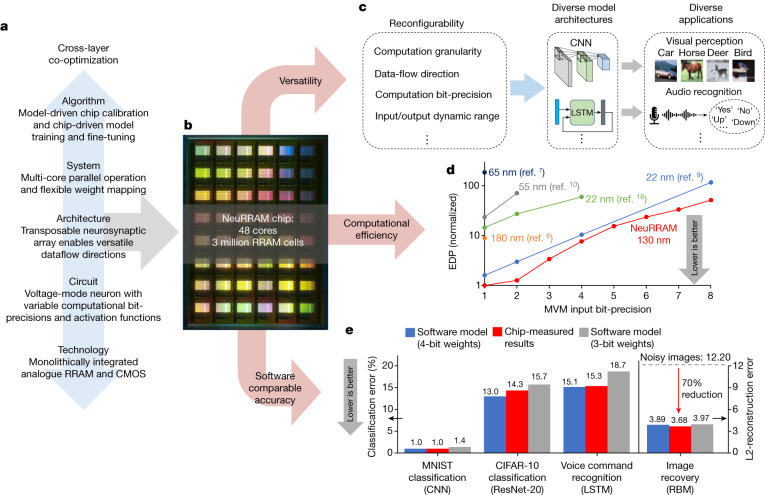
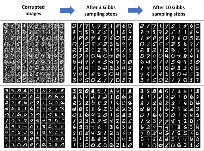
Abstract Realizing increasingly complex artificial intelligence (AI) functionalities directly on edge devices calls for unprecedented energy efficiency of edge hardware. Compute-in-memory (CIM) based on resistive random-access memory (RRAM) 1 promises to meet such demand by storing AI model weights in dense, analogue and non-volatile RRAM devices, and by performing AI computation directly within RRAM, thus eliminating power-hungry data movement between separate compute and memory 2–5 . Although recent studies have demonstrated in-memory matrix-vector multiplication on fully integrated RRAM-CIM hardware 6–17 , it remains a goal for a RRAM-CIM chip to simultaneously deliver high energy efficiency, versatility to support diverse models and software-comparable accuracy. Although efficiency, versatility and accuracy are all indispensable for broad adoption of the technology, the inter-related trade-offs among them cannot be addressed by isolated improvements on any single abstraction level of the design. Here, by co-optimizing across all hierarchies of the design from algorithms and architecture to circuits and devices, we present NeuRRAM—a RRAM-based CIM chip that simultaneously delivers versatility in reconfiguring CIM cores for diverse model architectures, energy efficiency that is two-times better than previous state-of-the-art RRAM-CIM chips across various computational bit-precisions, and inference accuracy comparable to software models quantized to four-bit weights across various AI tasks, including accuracy of 99.0 percent on MNIST 18 and 85.7 percent on CIFAR-10 19 image classification, 84.7-percent accuracy on Google speech command recognition 20 , and a 70-percent reduction in image-reconstruction error on a Bayesian image-recovery task.
Overview
CoChat Summary
TL;DR
NeuRRAM is a 48-core RRAM compute-in-memory chip that co-optimizes device, circuit, architecture, system, and algorithm choices to support reconfigurable AI inference with hardware-measured accuracy. The paper reports better energy-delay product than prior RRAM-CIM chips and benchmark results of 99.0% on MNIST, 85.7% on CIFAR-10, 84.7% on Google speech commands, and a 70% reduction in image-reconstruction error on MNIST image recovery.
Key findings
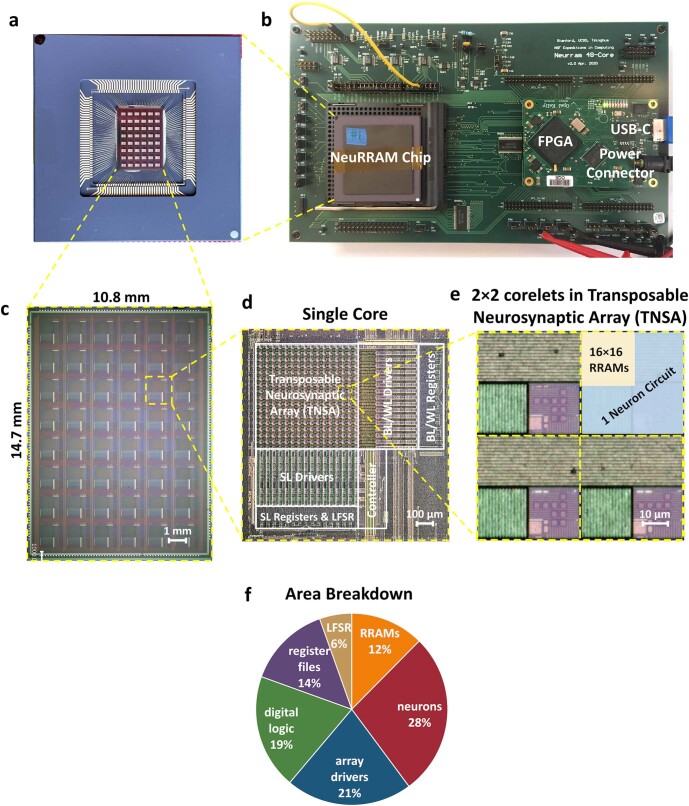
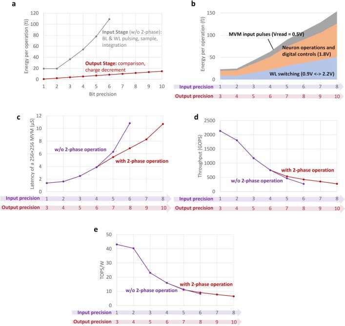
- The chip achieves an energy-delay product that is 1.6× to 2.3× lower than previous state-of-the-art RRAM-CIM chips, and 7× to 13× higher computational density at various MVM bit-precisions.
- Fully hardware-measured benchmark results include 99.0% MNIST accuracy, 85.7% CIFAR-10 accuracy, 84.7% Google speech command accuracy, and 70% lower image-reconstruction error on the Bayesian image-recovery task.
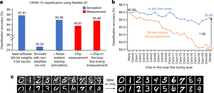
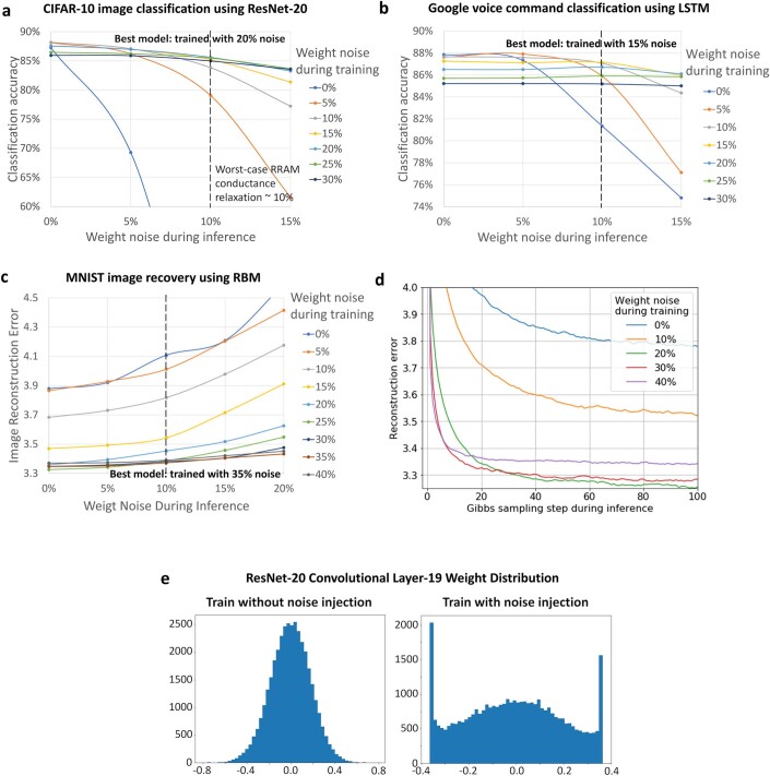
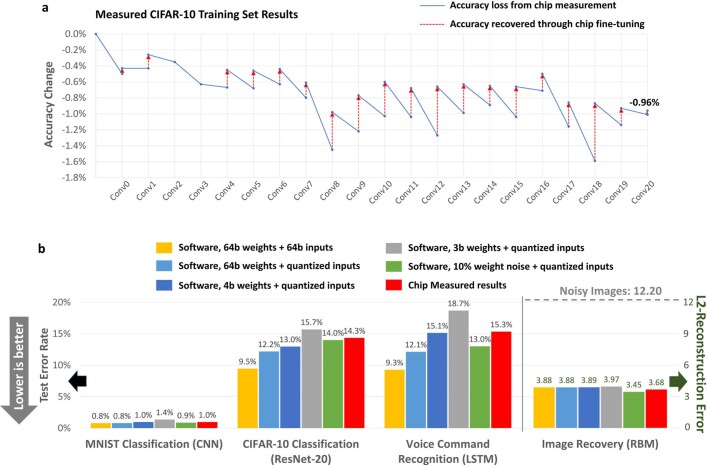
- Hardware-algorithm co-optimization improved CIFAR-10 classification from 25.34% accuracy without noise injection to 85.99% with noise injection; chip-in-the-loop progressive fine-tuning improved cumulative CIFAR-10 test-set accuracy by 1.99%.
- The authors report that the measured CIFAR-10 accuracy for deep ResNet-20 inference on-chip was 83.67%, which remained 3.36% below the 87.03% of the corresponding 4-bit-weight software model.
Methods
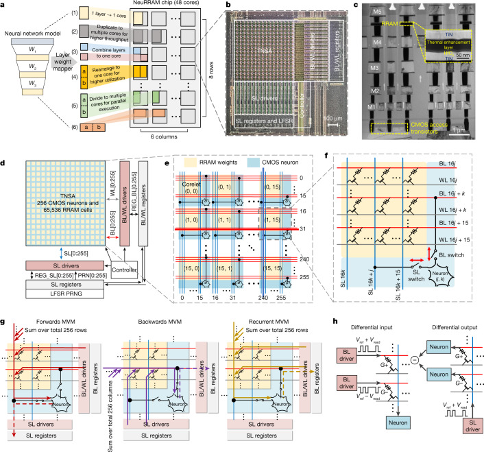
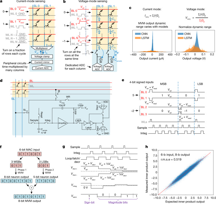
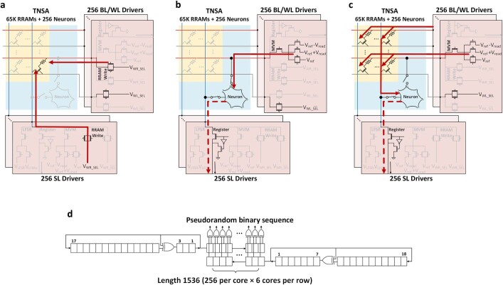
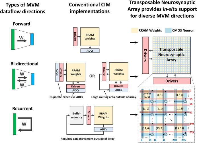
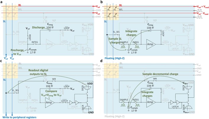
- Built a 48-core NeuRRAM chip with 3 million RRAM devices in a 130-nm CMOS process, using a bidirectional transposable neurosynaptic array (TNSA) and a voltage-mode neuron circuit.
- Evaluated the chip on multiple AI tasks: MNIST and CIFAR-10 image classification, Google speech command recognition, and MNIST image recovery with CNNs, LSTMs, and an RBM; all benchmark results were obtained from hardware measurements on complete datasets.
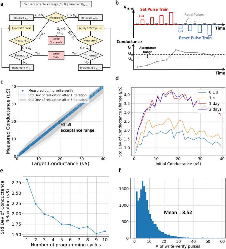
- Used model calibration, noise-resilient training, iterative write–verify programming, and chip-in-the-loop progressive fine-tuning; weights were mapped across cores with strategies for balancing load and mitigating voltage drop.
Limitations
- The paper states that the reported throughput and energy-efficiency numbers are peak values at 100% array utilization and do not include energy/time for buffering or moving intermediate data; this is an explicit limitation of the measurement scope.
- The paper notes that some on-chip accuracies are still below full-precision digital implementations, mainly because of ≤4-bit quantization of inputs and activations, especially sensitive input and output layers.
- Evident from the text: the implementation relies on an FPGA board for partial-sum accumulation, average pooling, buffers, and other operations, so the system is not a fully self-contained chip-level AI system in the demonstrated setup.
Model-written summary. Check it against the paper before relying on it.
Integrity signals
Registry
Cites
Statistics
Figures


Verification
Claims the paper makes
7 Valid · 1 Not valid · 7 Not checked · 130 Own results and interpretations
The cited sources support only part of this claim — read each source’s verdict below.
In the paper
“The accuracy gap mainly comes from low-precision (≤4-bit) quantization of inputs and activations, especially on the most sensitive input and output layers46.”
§ A compute-in-memory chip based on resistive random-access memory > Hardware-algorithm co-optimizations
What the sources say
- Partly supportedcites [46] Choi, J. et al. PACT: parameterized clipping activation for quantized neural networks. Preprint at https://arxiv.org/abs/1805.06085 (2018). sourceExperimental — accuracy not yet measured
Section A.3 (pp. 11–12) finds that aggressively quantizing the first or last layer can noticeably degrade accuracy, while using 8 bits for those layers causes little degradation in the tested model. Section 5.1 (p. 7) also finds that activation accuracy improves with precision. But it does not establish that the accuracy gap mainly comes from inputs and activations, and it reports less than a 1% validation-error difference when activation precision is at least 4 bits, so the claim’s ≤4-bit framing is too broad. (LLM, conf=0.86)
plainstates a cause- Asserted: passes — The authors put it forward as true.
- Checkable: passes — It can be checked against evidence.
- Load-bearing: passes — The paper’s conclusions depend on it.
- Based: passes — The paper gives a reason why it holds.
- Partly supported
The cited sources support only part of this claim — read each source’s verdict below.
In the paper
“The accuracies of some of our quantized models are lower than that of the state-of-the-art quantized model because we apply <4-bit quantization to the most sensitive input and output layers of the neural networks”
§ A compute-in-memory chip based on resistive random-access memory > Methods > Noise-resilient neural-network training
What the sources say
- Supportedcites [46] Choi, J. et al. PACT: parameterized clipping activation for quantized neural networks. Preprint at https://arxiv.org/abs/1805.06085 (2018). source
Section A.3 (pp. 11–12) reports that aggressively quantizing the first or last layer can noticeably degrade accuracy; its table shows substantially higher validation error when those layers use 2 bits. The comparison with a state-of-the-art model describes the citing authors’ own results, not a finding attributed to PACT. (LLM, conf=0.88)
- Not matchedcites [54] Esser, S. K., Mckinstry, J. L., Bablani, D., Appuswamy, R. & Modha, D. S. Learned step size quantization. In International Conference on Learning Representations (ICLR) (2020).
Couldn’t be matched to a paper in Crossref, so it can’t be checked.
plainstates a cause- Asserted: passes — The authors put it forward as true.
- Checkable: passes — It can be checked against evidence.
- Load-bearing: unclear — It is unclear whether the paper’s conclusions depend on it.
- Based: passes — The paper gives a reason why it holds.
- Supported
A result the paper reports from its own data — it cites no other source for it, so there is none to check. The quote shows it is in the paper.
In the paper
“we achieve a 0.98% error rate on MNIST handwritten digit recognition using a 7-layer CNN”
§ A compute-in-memory chip based on resistive random-access memory > Hardware-algorithm co-optimizations
plain- Asserted: passes — The authors put it forward as true.
- Checkable: passes — It can be checked against evidence.
- Load-bearing: passes — The paper’s conclusions depend on it.
- Based: passes — The paper gives a reason why it holds.
A result the paper states — it cites no source for it, so there is none to check. The quote shows it is in the paper.
In the paper
“Some of these numbers are not yet to the accuracies achieved by full-precision digital implementations.”
§ A compute-in-memory chip based on resistive random-access memory > Hardware-algorithm co-optimizations
plain- Asserted: passes — The authors put it forward as true.
- Checkable: passes — It can be checked against evidence.
- Load-bearing: unclear — It is unclear whether the paper’s conclusions depend on it.
- Based: passes — The paper gives a reason why it holds.
A result the paper reports from its own data — it cites no other source for it, so there is none to check. The quote shows it is in the paper.
In the paper
“a 14.34% error rate on CIFAR-10 object classification using ResNet-20”
§ A compute-in-memory chip based on resistive random-access memory > Hardware-algorithm co-optimizations
plain- Asserted: passes — The authors put it forward as true.
- Checkable: passes — It can be checked against evidence.
- Load-bearing: passes — The paper’s conclusions depend on it.
- Based: passes — The paper gives a reason why it holds.
72 more claims
Create a free account to see all 145 claims and every source verdict.
- Probably not a substantial claim. 37
- It may state two separate claims as one. 41
Claims other papers make about this one
Each is checked against this paper’s own text: does it say what the citing paper says it does?
The source backs part of the claim, not all of it — or backs it for a different population, condition or comparison.
In the citing paper
“So far, several groups and companies have claimed the realization of hybrid CMOS/memristor implementations of ANNs53–61, —from now on, memristive ANNs— with performance that is superior to that of fully-CMOS counterparts.”
From Hardware implementation of memristor-based artificial neural networks (2024) · cites this paper as [60]
Experimental — accuracy not yet measuredThe source backs part of the claim, not all of it — or backs it for a different population, condition or comparison.
In the citing paper
“Although several compute-in-memory or near-memory approaches based on SRAMs and digital compute35–38 have been presented in the literature, most of these do not address the energy and time costs of reloading weights, thus making direct side-by-side comparisons against NVM-based weight-stationary approaches difficult.”
From An analog-AI chip for energy-efficient speech recognition and transcription (2023) · cites this paper as [7]
Experimental — accuracy not yet measuredThe cited source says what the claim attributes to it.
In the citing paper
“Some groups prefer to incorporate a transistor in series to each MIM cell to obtain a better control over the currents through the device (i.e., improve conductance controllability and minimize sneak path currents)53–55,60,61,102,113,167,194,218–222,).”
From Hardware implementation of memristor-based artificial neural networks (2024) · cites this paper as [60]
The cited source says what the claim attributes to it.
In the citing paper
“Then, analogue VMM has been demonstrated both for binary inputs and weights218–220, as well as for binary inputs and analogue/multilevel weights60,85,105,217.”
From Hardware implementation of memristor-based artificial neural networks (2024) · cites this paper as [60]
The cited source says what the claim attributes to it.
In the citing paper
“These results imply that with better architecture, materials, and hardware-software co-design [161], in-memory computing can set new standards for parallel processing.”
From Brain-inspired computing systems: a systematic literature review (2024) · cites this paper as [161]
2 more claims about this paper
Create a free account to see every claim other papers make about this one.
Citations
Cites
Deep Residual Learning for Image Recognition
He, K., Zhang, X., Ren, S., & Sun, J. (2016) · 2016 IEEE Conference on Computer Vision and Pattern Recognition (CVPR) · doi:10.1109/cvpr.2016.90 · Cited by 235,474
Hochreiter, S., & Schmidhuber, J. (1997) · Neural Computation · doi:10.1162/neco.1997.9.8.1735 · Cited by 102,318
LeCun, Y., Bengio, Y., & Hinton, G. (2015) · Nature · doi:10.1038/nature14539 · Cited by 84,126
Gradient-based learning applied to document recognition
Lecun, Y., Bottou, L., Bengio, Y., & Haffner, P. (1998) · Proceedings of the IEEE · doi:10.1109/5.726791 · Cited by 58,805
Multilayer feedforward networks are universal approximators
Hornik, K., Stinchcombe, M., & White, H. (1989) · Neural Networks · doi:10.1016/0893-6080(89)90020-8 · Cited by 21,728
International Conference on Learning Representations (ICLR 2013)
松尾, 豊. (2013) · 人工知能学会誌 = Journal of Japanese Society for Artificial Intelligence · Cited by 6,286
In-Datacenter Performance Analysis of a Tensor Processing Unit
Jouppi, N. P., Young, C., Patil, N., Patterson, D., Agrawal, G., Bajwa, R., Bates, S., Bhatia, S., Boden, N., Borchers, A., et al. (2017) · Proceedings of the 44th Annual International Symposium on Computer Architecture · doi:10.1145/3079856.3080246 · Cited by 4,537
Eyeriss: An Energy-Efficient Reconfigurable Accelerator for Deep Convolutional Neural Networks
Chen, Y.-H., Krishna, T., Emer, J. S., & Sze, V. (2017) · IEEE Journal of Solid-State Circuits · doi:10.1109/jssc.2016.2616357 · Cited by 3,247
Training and operation of an integrated neuromorphic network based on metal-oxide memristors
Prezioso, M., Merrikh-Bayat, F., Hoskins, B. D., Adam, G. C., Likharev, K. K., & Strukov, D. B. (2015) · Nature · doi:10.1038/nature14441 · Cited by 3,001 · cited 2×
“…based on resistive random-access memory (RRAM) 1 promises to meet such demand by storing AI model weights in dense, analogue and non-volatile RRAM devices, and by performing AI computation directly within RRAM, thus eliminating power-hungry data movement between separate compute and memory 2–5 .”
Wong, H.-S. P., Lee, H.-Y., Yu, S., Chen, Y.-S., Wu, Y., Chen, P.-S., Lee, B., Chen, F. T., & Tsai, M.-J. (2012) · Proceedings of the IEEE · doi:10.1109/jproc.2012.2190369 · Cited by 2,757
Self-citation
Research works printed but not linked: 1
- Koller, D. & Friedman, N. Probabilistic Graphical Models: Principles and Techniques (Adaptive Computation and Machine Learning series) (MIT Press, 2009).
Cited by
Hardware implementation of memristor-based artificial neural networks
Aguirre, F., Sebastian, A., Le Gallo, M., Song, W., Wang, T., Yang, J. J., Lu, W., Chang, M.-F., Ielmini, D., Yang, Y., et al. (2024) · Nature Communications · doi:10.1038/s41467-024-45670-9 · Cited by 564
“Also, many papers 55,60,99,100 , have explored the case of ANNs with binarized inputs, as they employ the simplest DACs (1-bit).”
Thousands of conductance levels in memristors integrated on CMOS
(2023) · doi:10.1038/s41586-023-05759-5 · Cited by 503
Memristor‐Based Neuromorphic Chips
Duan, X., Cao, Z., Gao, K., Yan, W., Sun, S., Zhou, G., Wu, Z., Ren, F., & Sun, B. (2024) · Advanced Materials · doi:10.1002/adma.202310704 · Cited by 432
Neuromorphic computing at scale
Kudithipudi, D., Schuman, C., Vineyard, C. M., Pandit, T., Merkel, C., Kubendran, R., Aimone, J. B., Orchard, G., Mayr, C., Benosman, R., et al. (2025) · Nature · doi:10.1038/s41586-024-08253-8 · Cited by 357
“Several emergent devices have addressed device non-idealities by using some form of online training 121,146,157 .”
Self-citationLe Gallo, M., Khaddam-Aljameh, R., Stanisavljevic, M., Vasilopoulos, A., Kersting, B., Dazzi, M., Karunaratne, G., Brändli, M., Singh, A., Müller, S. M., et al. (2023) · Nature Electronics · doi:10.1038/s41928-023-01010-1 · Cited by 310
Metadata
- Authors
- Wan, W., Kubendran, R., Schaefer, C., Eryilmaz, S. B., Zhang, W., Wu, D., Deiss, S., Raina, P., Qian, H., Gao, B., Joshi, S., Wu, H., Wong, H.-S. P., & Cauwenberghs, G.
- Affiliations
- University of California San Diego (US)
- University of Pittsburgh (US)
- University of Notre Dame (US)
- Stanford University (US)
- Tsinghua University (CN)
- Corresponding author
- Wan, Weier
- Gao, Bin
- Joshi, Siddharth
- Wu, Huaqiang
- Wong, H.-S. Philip
- Cauwenberghs, Gert
- ORCID
- Venue
- Nature
- Published
- 2022-08-17
- Volume
- 608
- Issue
- 7923
- Pages
- 504-512
- ISSN
- 0028-0836 (ISSN-L)
- 1476-4687
- PMC
- PMC9385482
- OpenAlex
- W4292121737
- Cited by
- 943
- References
- 65
- Citations by year
- 2026: 235 · 2025: 273 · 2024: 246 · 2023: 167 · 2022: 22
- FWCI
- 48.45
- Type
- journal article
- Language
- en
- Open access
- hybrid
- doi.org
- Licence
- cc-by
- creativecommons.org/licenses/by/4.0 (tdm)
- creativecommons.org/licenses/by/4.0 (vor)
- Locations
- Nature (publishedVersion, cc-by)
- PubMed Central (publishedVersion, cc-by)
- PubMed (publishedVersion)
- RePEc: Research Papers in Economics (submittedVersion)
- eScholarship (California Digital Library) (submittedVersion, cc-by)
- Funders
- National Science Foundation (1317470)
- Western Digital
- University of Pennsylvania
- Pennsylvania State University
- Stanford SystemX Alliance
- National Natural Science Foundation of China (61851404)
- Office of Naval Research
- Topics
- Physical Sciences › Engineering › Electrical and Electronic Engineering › Advanced Memory and Neural Computing
- Physical Sciences › Engineering › Electrical and Electronic Engineering › Ferroelectric and Negative Capacitance Devices
- Physical Sciences › Computer Science › Computer Vision and Pattern Recognition › Advanced Neural Network Applications
- Keywords
- in-memory computing, resistive random access memory, neuromorphic hardware, edge AI, energy efficiency, weight quantization, hardware-software co-optimization, non-volatile memory, image classification, voice command recognition
About these checks
Registry, retraction, Cites and statistics results are computed, not judged, with one exception: a printed reference that no index lists is read once by a model before it counts as a citation error. Claims are extracted by a model and kept only when their quote appears verbatim in the text; each cited source is then checked, with a model’s help, for whether it says what the claim relies on. Those verdicts can be wrong — read the claim’s quote and the cited source before relying on one.
The claim verdicts this report counts are experimental: their accuracy is not yet measured.
A language model drew the claims from the paper on 2026-09-29, under version 3 of the claim definition (model deepseek-v4.1-flash, prompt extract-v3).
A second model labelled each claim on 2026-09-29 (model jev-1.13-20260917, definition revision gold-guideline-v0.2).
Cited sources are checked with a language model’s help (gpt-6-sol).
Statistics and arithmetic are recomputed, not judged.
Confidence bands are shown only for fields calibrated on our annotated test set. None is calibrated yet, so no band is shown.
What counts as a claim ›How we measure confidence ›How we check this ›
Are you an author, or do you see a problem with this page? Request a review
How to cite
Cite CoChat for the checks on this page, and the paper for its own findings.
- This page
- CoChat. (2026). Citation check: A compute-in-memory chip based on resistive random-access memory. https://app.cochat.ai/papers/10.1038/s41586-022-04992-8
- The paper
- Wan, W., Kubendran, R., Schaefer, C., Eryilmaz, S. B., Zhang, W., Wu, D., Deiss, S., Raina, P., Qian, H., Gao, B., Joshi, S., Wu, H., Wong, H.-S. P., & Cauwenberghs, G. (2022). A compute-in-memory chip based on resistive random-access memory. Nature. https://doi.org/10.1038/s41586-022-04992-8
Data sources
Bibliographic data: Semantic Scholar, OpenAlex, Crossref.
Contains information from the Semantic Scholar Academic Graph Datasets, made available under the ODC Attribution License (ODC-BY 1.0).
Semantic Scholar’s data is described in: Kinney, R., et al. (2023). The Semantic Scholar Open Data Platform. arXiv:2301.10140.
