

The DOI matches its Crossref record; 60 of the 63 references it cites were found in a registry or an index; none of the 31 sources its claims cite is checked for support yet.
Socioeconomic status determines COVID-19 incidence and related mortality in Santiago, Chile
Open accessPublished version of a preprint
Abstract
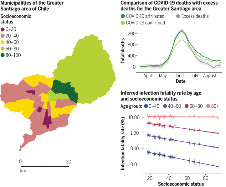
Urban socioeconomics and mortality: Santiago, Chile, is a highly segregated city with distinct zones of affluence and deprivation. This setting offers a window on how social factors propel the severe acute respiratory syndrome coronavirus 2 (SARS-CoV-2) pandemic in an economically vulnerable society with high levels of income inequality. Mena et al. analyzed incidence and mortality attributed to SARS-CoV-2 to understand spatial variations in disease burden. Infection fatality rates were higher in lower-income municipalities because of comorbidities and lack of access to health care. Disparities between municipalities in the quality of their health care delivery system became apparent in testing delays and capacity. These indicators explain a large part of the variation in COVID-19 underreporting and deaths and show that these inequalities disproportionately affected younger people. Science , abg5298, this issue p. eabg5298
Overview
AI snapshot
Written from the paper’s full text.
TL;DR
In Greater Santiago, Chile, COVID-19 incidence, mortality, testing delays, and infection fatality rates were strongly patterned by municipal socioeconomic status, with lower-SES areas experiencing higher burden and younger-age mortality. The authors link these disparities to mobility constraints, early underreporting, and unequal health care capacity.
Key findings
- SES ranged from Vitacura (93.7) to La Pintana (17.0). Maximum weekly incidence was 22.6 cases per 10,000 in Vitacura in mid-May versus 76.4 in La Pintana in the first week of June; maximum weekly deaths were 4.4 per 10,000 in San Ramón (SES 19.7) versus 1.6 in Vitacura in June.
- During full lockdown, the two highest-SES municipalities reduced mobility by up to 61%, whereas lowest-SES municipalities reduced mobility on average to 40%.
- Observed deaths in May–July 2020 were more than 1.73 times expected (CI 1.68–1.79), peaking above 2110 deaths in epidemiological week 24 versus an expected 802 deaths and an average of 798 deaths between 2015 and 2019. Age-specific observed deaths were nearly twofold higher for people younger than 40, 2.8 times higher for ages 40–60, 3.2 times higher for ages 60–80, and 2.4 times higher for ages 80+.
- Low- versus high-SES IFR ratios were 1.4 for ages 60–80, 1.7 for ages 40–60, and 3.1 for ages 0–40. Positivity was negatively associated with SES, timeliness was associated with SES, and tests per death were positively associated with SES; South and West zones had four times fewer beds per 10,000 people and four times lower private health system enrollment than the East zone, and more than 90% of COVID-19–attributed deaths in South and West zones occurred outside health care facilities versus 55% in the East zone.
Methods
- Ecological analysis of 34 municipalities in Greater Santiago, home to almost 7 million people, using SES defined as 100 − the 2019 social priority index (SPI), COVID-19 data from the EPIVIGILA platform, vital statistics mortality data, and Facebook Data for Good mobility data.
- RmMAP, a Poisson deconvolution model with a quadratic penalty, back-calculated infections from COVID-19–attributed deaths and an onset-to-death distribution; Gaussian process regression estimated excess deaths using 2000–2019 mortality data; a hierarchical Bayesian model inferred CFR/IFR by age and municipality from cases, positivity, deaths, and SES.
- Analyses related SES to incidence, age-adjusted death rates, mobility, testing positivity, timeliness, and tests per death, and compared IFR ratios across low, mid-low, mid-high, and high SES categories.
Limitations
- The paper states that mobile phone mobility data are likely biased because of differential mobile phone ownership across demographic groups, though results were consistent with other Santiago studies using different measurements.
- The paper states that RmMAP estimates rely on the infection-to-death distribution and assume IFRs do not change over time; excess mortality estimates depend on kernel choice; and IFR estimates rely on Bayesian assumptions about reporting rates and age distribution of infections, with sensitivity analyses suggesting stability.
- Evident from the text: the study is observational and ecological, using municipality-level SES and aggregated data, so it cannot establish causality; age information of reported cases was not available at the municipality level.
Model-written summary. Check it against the paper before relying on it.
Integrity signals
Registry
Cites
Statistics
Figures
Verification
Claims the paper makes
40 Own result · 16 Not checked yet · 16 Own interpretation · 7 Own method · 6 No basis given
A result the paper reports from its own data — it cites no other source for it, so there is none to check. The quote shows it is in the paper.
In the paper
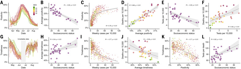
“As shown in Fig. 4G, timeliness follows a similar temporal course as test positivity during May and part of June, but in the opposite direction.”
§ Socioeconomic status determines COVID-19 incidence and related mortality in Santiago, Chile > More testing with lower waiting times in wealthy areas
plaincorrelational- Asserted: passes — The authors put it forward as true.
- Checkable: passes — It can be checked against evidence.
- Load-bearing: unclear — It is unclear whether the paper’s conclusions depend on it.
- Based: passes — The paper gives a reason why it holds.
A result the paper reports from its own data — it cites no other source for it, so there is none to check. The quote shows it is in the paper.
In the paper
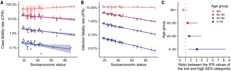
“The difference is even more pronounced in the younger age group (0 to 40 years old), which shows values of IFR that are 3.1 times higher for the municipalities with the lowest SES.”
§ Socioeconomic status determines COVID-19 incidence and related mortality in Santiago, Chile > IFR depends on SES
plaincorrelational- Asserted: passes — The authors put it forward as true.
- Checkable: passes — It can be checked against evidence.
- Load-bearing: passes — The paper’s conclusions depend on it.
- Based: passes — The paper gives a reason why it holds.
A result the paper reports from its own data — it cites no other source for it, so there is none to check. The quote shows it is in the paper.
In the paper
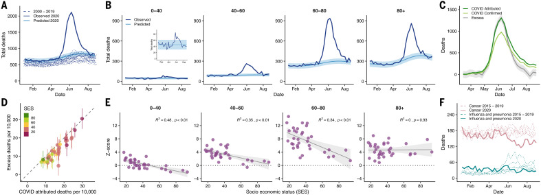
“In addition, lower numbers of deaths were reported for respiratory infectious diseases, such as influenza and pneumonia, and cancer during July and August 2020 compared with the period from 2015 to 2019 (Fig. 3F).”
§ Socioeconomic status determines COVID-19 incidence and related mortality in Santiago, Chile > Excess deaths match COVID-19–attributed deaths
plain- Asserted: passes — The authors put it forward as true.
- Checkable: passes — It can be checked against evidence.
- Load-bearing: unclear — It is unclear whether the paper’s conclusions depend on it.
- Based: passes — The paper gives a reason why it holds.
A result the paper reports from its own data — it cites no other source for it, so there is none to check. The quote shows it is in the paper.
In the paper
“which also shows COVID-19–attributed deaths higher than the excess deaths in most of the cases.”
§ Socioeconomic status determines COVID-19 incidence and related mortality in Santiago, Chile > Excess deaths match COVID-19–attributed deaths
plain- Asserted: passes — The authors put it forward as true.
- Checkable: passes — It can be checked against evidence.
- Load-bearing: unclear — It is unclear whether the paper’s conclusions depend on it.
- Based: passes — The paper gives a reason why it holds.
A result the paper reports from its own data — it cites no other source for it, so there is none to check. The quote shows it is in the paper.
In the paper
“Disparities between municipalities in the quality of their health care delivery system became apparent in testing delays and capacity.”
§ Socioeconomic status determines COVID-19 incidence and related mortality in Santiago, Chile > Abstract
plaincorrelational- Asserted: passes — The authors put it forward as true.
- Checkable: passes — It can be checked against evidence.
- Load-bearing: passes — The paper’s conclusions depend on it.
- Based: passes — The paper gives a reason why it holds.
A result the paper reports from its own data — it cites no other source for it, so there is none to check. The quote shows it is in the paper.
In the paper
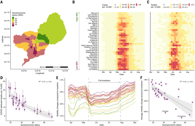
“we show that the two municipalities with highest SES exhibited a reduction in mobility by up to 61% during the full lockdown (dark green regions in Fig. 1E) compared with the ones with lowest SES, which, on average, reduced their mobility to 40% during the this period (dark pink regions in Fig. 1E).”
§ Socioeconomic status determines COVID-19 incidence and related mortality in Santiago, Chile > Association between socioeconomic status and disease dynamics
plaincorrelational- Asserted: passes — The authors put it forward as true.
- Checkable: passes — It can be checked against evidence.
- Load-bearing: passes — The paper’s conclusions depend on it.
- Based: passes — The paper gives a reason why it holds.
- Rests on an assumption: Human mobility indicators inferred from anonymized mobile phone data are a valid proxy for physical distancing.
A result the paper reports from its own data — it cites no other source for it, so there is none to check. The quote shows it is in the paper.
In the paper
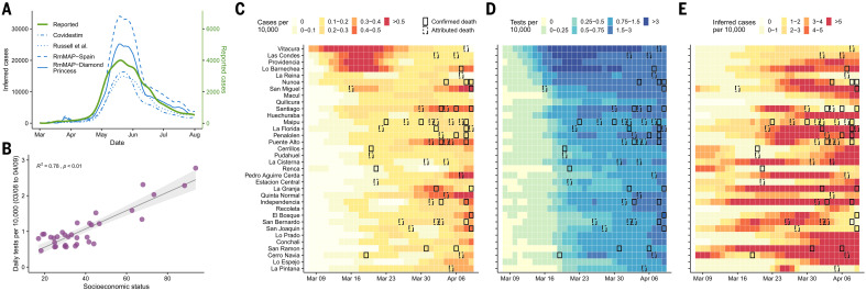
“We analyzed the number of tests performed between 8 March and 9 April and find a significantly higher number of tests performed in municipalities with high SES (Fig. 2B), especially during the first 2 weeks of March (Fig. 2D).”
§ Socioeconomic status determines COVID-19 incidence and related mortality in Santiago, Chile > Epidemic reconstruction reveals early transmission dynamics
plaincorrelational- Asserted: passes — The authors put it forward as true.
- Checkable: passes — It can be checked against evidence.
- Load-bearing: passes — The paper’s conclusions depend on it.
- Based: passes — The paper gives a reason why it holds.
A result the paper reports from its own data — it cites no other source for it, so there is none to check. The quote shows it is in the paper.
In the paper
“This metric is associated with SES, suggesting that municipalities with low SES, on average, get their test results later than the ones with high SES (Fig. 4H).”
§ Socioeconomic status determines COVID-19 incidence and related mortality in Santiago, Chile > More testing with lower waiting times in wealthy areas
hedgedcorrelational- Asserted: passes — The authors put it forward as true.
- Checkable: passes — It can be checked against evidence.
- Load-bearing: passes — The paper’s conclusions depend on it.
- Based: passes — The paper gives a reason why it holds.
A result the paper reports from its own data — it cites no other source for it, so there is none to check. The quote shows it is in the paper.
In the paper
“Furthermore, the two municipalities with a SES higher than 80 (Las Condes and Vitacura) had z scores of much smaller magnitude (with the exception of the oldest age group), indicating that in those areas, patterns of mortality did not deviate much from what would have been expected for a normal year in people younger than 80 years old.”
§ Socioeconomic status determines COVID-19 incidence and related mortality in Santiago, Chile > Excess deaths match COVID-19–attributed deaths
hedged- Asserted: passes — The authors put it forward as true.
- Checkable: passes — It can be checked against evidence.
- Load-bearing: unclear — It is unclear whether the paper’s conclusions depend on it.
- Based: passes — The paper gives a reason why it holds.
A result the paper reports from its own data — it cites no other source for it, so there is none to check. The quote shows it is in the paper.
In the paper
“with an estimate of the number of infected individuals that is 5 to 10 times greater than the reported values.”
§ Socioeconomic status determines COVID-19 incidence and related mortality in Santiago, Chile > Epidemic reconstruction reveals early transmission dynamics
hedged- Asserted: passes — The authors put it forward as true.
- Checkable: passes — It can be checked against evidence.
- Load-bearing: passes — The paper’s conclusions depend on it.
- Based: passes — The paper gives a reason why it holds.
A result the paper reports from its own data — it cites no other source for it, so there is none to check. The quote shows it is in the paper.
In the paper
“When comparing the IFR ratio between the low- and the high-SES categories, the results show a significantly higher IFR in the low-SES group in people younger than 80 years old (Fig. 5C).”
§ Socioeconomic status determines COVID-19 incidence and related mortality in Santiago, Chile > IFR depends on SES
plaincorrelational- Asserted: passes — The authors put it forward as true.
- Checkable: passes — It can be checked against evidence.
- Load-bearing: passes — The paper’s conclusions depend on it.
- Based: passes — The paper gives a reason why it holds.
A result the paper reports from its own data — it cites no other source for it, so there is none to check. The quote shows it is in the paper.
In the paper
“This relationship between reductions in mobility and SES was present during all time periods considered for this study (Fig. 1F)”
§ Socioeconomic status determines COVID-19 incidence and related mortality in Santiago, Chile > Association between socioeconomic status and disease dynamics
plaincorrelational- Asserted: passes — The authors put it forward as true.
- Checkable: passes — It can be checked against evidence.
- Load-bearing: passes — The paper’s conclusions depend on it.
- Based: passes — The paper gives a reason why it holds.
- Rests on an assumption: Human mobility indicators inferred from anonymized mobile phone data are a valid proxy for physical distancing.
A result the paper reports from its own data — it cites no other source for it, so there is none to check. The quote shows it is in the paper.
In the paper
“Our RmMAP estimates at the municipality level support this claim, because they capture a high volume of early infections in most municipalities (Fig. 2E), a scenario that largely deviates from the official tallies (Fig. 2C).”
§ Socioeconomic status determines COVID-19 incidence and related mortality in Santiago, Chile > Epidemic reconstruction reveals early transmission dynamics
plaincorrelational- Asserted: passes — The authors put it forward as true.
- Checkable: passes — It can be checked against evidence.
- Load-bearing: passes — The paper’s conclusions depend on it.
- Based: passes — The paper gives a reason why it holds.
A result the paper reports from its own data — it cites no other source for it, so there is none to check. The quote shows it is in the paper.
In the paper
“With the exception of the oldest age group, CFR shows a negative association with SES.”
§ Socioeconomic status determines COVID-19 incidence and related mortality in Santiago, Chile > IFR depends on SES
plaincorrelational- Asserted: passes — The authors put it forward as true.
- Checkable: passes — It can be checked against evidence.
- Load-bearing: passes — The paper’s conclusions depend on it.
- Based: passes — The paper gives a reason why it holds.
A result the paper reports from its own data — it cites no other source for it, so there is none to check. The quote shows it is in the paper.
In the paper
“We do not observe a substantial contribution from these causes (see supplementary materials, along with additional detailed analyses).”
§ Socioeconomic status determines COVID-19 incidence and related mortality in Santiago, Chile > Excess deaths match COVID-19–attributed deaths
plain- Asserted: passes — The authors put it forward as true.
- Checkable: passes — It can be checked against evidence.
- Load-bearing: unclear — It is unclear whether the paper’s conclusions depend on it.
- Based: passes — The paper gives a reason why it holds.
A result the paper reports from its own data — it cites no other source for it, so there is none to check. The quote shows it is in the paper.
In the paper
“As shown in Fig. 1C and fig. S1, the attributed COVID-19 deaths follow a similar (yet lagged) temporal pattern to the number of reported COVID-19 cases.”
§ Socioeconomic status determines COVID-19 incidence and related mortality in Santiago, Chile > Association between socioeconomic status and disease dynamics
plaincorrelational- Asserted: passes — The authors put it forward as true.
- Checkable: passes — It can be checked against evidence.
- Load-bearing: unclear — It is unclear whether the paper’s conclusions depend on it.
- Based: passes — The paper gives a reason why it holds.
A result the paper reports from its own data — it cites no other source for it, so there is none to check. The quote shows it is in the paper.
In the paper
“Second, our analyses revealed an underreporting of infections in low-income areas at the start of the outbreak.”
§ Socioeconomic status determines COVID-19 incidence and related mortality in Santiago, Chile > Discussion
plain- Asserted: passes — The authors put it forward as true.
- Checkable: passes — It can be checked against evidence.
- Load-bearing: passes — The paper’s conclusions depend on it.
- Based: passes — The paper gives a reason why it holds.
The paper states this without a source or data behind it here, so there is nothing to check it against. The quote shows it is in the paper.
In the paper
“Finally, IFRs were higher in lower-SES municipalities, especially among younger people.”
§ Socioeconomic status determines COVID-19 incidence and related mortality in Santiago, Chile > Discussion
plaincorrelational- Asserted: passes — The authors put it forward as true.
- Checkable: passes — It can be checked against evidence.
- Load-bearing: passes — The paper’s conclusions depend on it.
- Based: passes — The paper gives a reason why it holds.
What the paper did — it cites no source for this, so there is none to check. The quote shows it is in the paper.
In the paper
“Our estimates of CFR have been validated by the official ICOVID platform (www.icovidchile.cl/), which confirmed that 119 out of the 136 observed CFRs fall within our confidence intervals.”
§ Socioeconomic status determines COVID-19 incidence and related mortality in Santiago, Chile > IFR depends on SES
plain- Asserted: passes — The authors put it forward as true.
- Checkable: passes — It can be checked against evidence.
- Load-bearing: unclear — It is unclear whether the paper’s conclusions depend on it.
- Based: passes — The paper gives a reason why it holds.
A conclusion the paper draws from its own results — it cites no other source for it, so there is none to check. The quote shows it is in the paper.
In the paper
“show that these inequalities disproportionately affected younger people.”
§ Socioeconomic status determines COVID-19 incidence and related mortality in Santiago, Chile > Abstract
plaincorrelational- Asserted: passes — The authors put it forward as true.
- Checkable: passes — It can be checked against evidence.
- Load-bearing: passes — The paper’s conclusions depend on it.
- Based: passes — The paper gives a reason why it holds.
In the paper
“Although confirmed COVID-19 cases are an important public health measure to estimate the level of spread of infections caused by SARS-CoV-2, they may not be a reliable indicator of incidence because of biases due to population-level health-seeking behavior, surveillance capacities, and the presence of asymptomatic individuals across regions (6).”
§ Socioeconomic status determines COVID-19 incidence and related mortality in Santiago, Chile > Abstract
What the sources say
- Not checked yetcites [6] F. S. Lu, A. T. Nguyen, N. B. Link, J. T. Davis, M. Chinazzi, X. Xiong, A. Vespignani, M. Lipsitch, M. Santillana, Estimating the cumulative incidence of COVID-19 in the United States using four complementary approaches. medRxiv 2020.04.18.20070821 [Preprint]. 7 August 2020; 10.1101/2020.04.18.20070821 PMC8241061 34138845
hedgedconditional- Asserted: passes — The authors put it forward as true.
- Checkable: passes — It can be checked against evidence.
- Load-bearing: passes — The paper’s conclusions depend on it.
- Based: passes — The paper gives a reason why it holds.
A conclusion the paper draws from its own results — it cites no other source for it, so there is none to check. The quote shows it is in the paper.
In the paper
“supports the hypothesis that people in poorer regions cannot afford to stay at home during lockdowns.”
§ Socioeconomic status determines COVID-19 incidence and related mortality in Santiago, Chile > Association between socioeconomic status and disease dynamics
hedgeddirect- Asserted: passes — The authors put it forward as true.
- Checkable: passes — It can be checked against evidence.
- Load-bearing: passes — The paper’s conclusions depend on it.
- Based: passes — The paper gives a reason why it holds.
The paper states this without a source or data behind it here, so there is nothing to check it against. The quote shows it is in the paper.
In the paper
“This is in part because ascertainment biases may be less pronounced for deaths than for confirmed cases, because people dying from COVID-19 are more likely to have experienced severe symptoms and thus are more likely to have been documented as COVID-19–positive cases by health surveillance systems.”
§ Socioeconomic status determines COVID-19 incidence and related mortality in Santiago, Chile > Abstract
hedgedconditional- Asserted: passes — The authors put it forward as true.
- Checkable: passes — It can be checked against evidence.
- Load-bearing: passes — The paper’s conclusions depend on it.
- Based: passes — The paper gives a reason why it holds.
A conclusion the paper draws from its own results — it cites no other source for it, so there is none to check. The quote shows it is in the paper.
In the paper
“These social inequalities affect the overall COVID-19 mortality rates, as shown in Fig. 1D.”
§ Socioeconomic status determines COVID-19 incidence and related mortality in Santiago, Chile > Association between socioeconomic status and disease dynamics
plaindirect- Asserted: passes — The authors put it forward as true.
- Checkable: passes — It can be checked against evidence.
- Load-bearing: passes — The paper’s conclusions depend on it.
- Based: passes — The paper gives a reason why it holds.
None of the sources cited for this claim have been checked yet.
In the paper
“Analyses of COVID-19–related deaths as well as excess mortality provide an alternative and potentially less biased picture of epidemic intensity (7, 8).”
§ Socioeconomic status determines COVID-19 incidence and related mortality in Santiago, Chile > Abstract
What the sources say
- Not checked yetcites [7] D. M. Weinberger, J. Chen, T. Cohen, F. W. Crawford, F. Mostashari, D. Olson, V. E. Pitzer, N. G. Reich, M. Russi, L. Simonsen, A. Watkins, C. Viboud, Estimation of excess deaths associated with the COVID-19 pandemic in the United States, March to May 2020. JAMA Intern. Med. 180, 1336– 1344 (2020). 10.1001/jamainternmed.2020.3391 32609310 PMC7330834 source
- Not checked yetcites [8] R. J. Acosta, R. A. Irizarry, Monitoring health systems by estimating excess mortality. medRxiv 2020.06.06.20120857 [Preprint]. 9 June 2020;. 10.1101/2020.06.06.20120857
hedged- Asserted: passes — The authors put it forward as true.
- Checkable: passes — It can be checked against evidence.
- Load-bearing: passes — The paper’s conclusions depend on it.
- Based: passes — The paper gives a reason why it holds.
A conclusion the paper draws from its own results — it cites no other source for it, so there is none to check. The quote shows it is in the paper.
In the paper
“These indicators explain a large part of the variation in COVID-19 underreporting and deaths”
§ Socioeconomic status determines COVID-19 incidence and related mortality in Santiago, Chile > Abstract
plaincorrelational- Asserted: passes — The authors put it forward as true.
- Checkable: passes — It can be checked against evidence.
- Load-bearing: passes — The paper’s conclusions depend on it.
- Based: passes — The paper gives a reason why it holds.
In the paper
“This early underreporting signal suggests that the patterns of mortality and testing observed across Greater Santiago are partially explained by an early failure of health care systems in informing the population with sufficient situational awareness about the real magnitude of the threat (15).”
§ Socioeconomic status determines COVID-19 incidence and related mortality in Santiago, Chile > Epidemic reconstruction reveals early transmission dynamics
What the sources say
- Not checked yetcites [15] M. Lipsitch, M. Santillana, “Enhancing situational awareness to prevent infectious disease outbreaks from becoming catastrophic” in Global Catastrophic Biological Risks, T. V. Inglesby, A. A. Adalja, Eds. (Current Topics in Microbiology and Immunology, vol. 424, Springer, 2019), pp. 59–74. 31292726 source
hedgedconditional- Asserted: passes — The authors put it forward as true.
- Checkable: passes — It can be checked against evidence.
- Load-bearing: unclear — It is unclear whether the paper’s conclusions depend on it.
- Based: passes — The paper gives a reason why it holds.
A conclusion the paper draws from its own results — it cites no other source for it, so there is none to check. The quote shows it is in the paper.
In the paper
“Although the observation that COVID-19–attributed deaths are greater than the estimated excess deaths might be counterintuitive (Fig. 3D), it may indicate the presence of changes in overall mortality patterns due to other causes, including a lower number of deaths attributable to a reduction in mobility.”
§ Socioeconomic status determines COVID-19 incidence and related mortality in Santiago, Chile > Excess deaths match COVID-19–attributed deaths
hedgedconditional- Asserted: passes — The authors put it forward as true.
- Checkable: passes — It can be checked against evidence.
- Load-bearing: unclear — It is unclear whether the paper’s conclusions depend on it.
- Based: passes — The paper gives a reason why it holds.
In the paper
“Changes in mortality from respiratory diseases can be explained by a mild influenza season in the Southern Hemisphere during the winter of 2020 (18)”
§ Socioeconomic status determines COVID-19 incidence and related mortality in Santiago, Chile > Excess deaths match COVID-19–attributed deaths
What the sources say
- Not checked yetcites [18] S. J. Olsen, E. Azziz-Baumgartner, A. P. Budd, L. Brammer, S. Sullivan, R. F. Pineda, C. Cohen, A. M. Fry, Decreased influenza activity during the COVID-19 pandemic-United States, Australia, Chile, and South Africa, 2020. Am. J. Transplant. 20, 3681– 3685 (2020). 10.1111/ajt.16381 33264506 PMC7753605 source
plaindirect- Asserted: passes — The authors put it forward as true.
- Checkable: passes — It can be checked against evidence.
- Load-bearing: unclear — It is unclear whether the paper’s conclusions depend on it.
- Based: passes — The paper gives a reason why it holds.
In the paper
“Second, more vulnerable communities may experience a higher prevalence of the comorbidities (31) that are associated with more severe presentations of COVID-19.”
§ Socioeconomic status determines COVID-19 incidence and related mortality in Santiago, Chile > Discussion
What the sources say
- Not checked yetcites [31] S. V. Subramanian, I. Delgado, L. Jadue, J. Vega, I. Kawachi, Income inequality and health: Multilevel analysis of Chilean communities. J. Epidemiol. Community Health 57, 844– 848 (2003). 10.1136/jech.57.11.844 14600107 PMC1732331 source
hedgedconditional- Asserted: passes — The authors put it forward as true.
- Checkable: passes — It can be checked against evidence.
- Load-bearing: passes — The paper’s conclusions depend on it.
- Based: passes — The paper gives a reason why it holds.
None of the sources cited for this claim have been checked yet.
In the paper
“Estimates of I maximizing Eq. 1 can be obtained with an expectation maximization algorithm (6, 33–35), but the outcome is typically unstable (36).”
§ Socioeconomic status determines COVID-19 incidence and related mortality in Santiago, Chile > Materials and methods > Models
What the sources say
- Not checked yetcites [6] F. S. Lu, A. T. Nguyen, N. B. Link, J. T. Davis, M. Chinazzi, X. Xiong, A. Vespignani, M. Lipsitch, M. Santillana, Estimating the cumulative incidence of COVID-19 in the United States using four complementary approaches. medRxiv 2020.04.18.20070821 [Preprint]. 7 August 2020; 10.1101/2020.04.18.20070821 PMC8241061 34138845 source
- Not checked yetcites [33] L. A. Shepp, Y. Vardi, Maximum likelihood reconstruction for emission tomography. IEEE Trans. Med. Imaging 1, 113– 122 (1982). 10.1109/TMI.1982.4307558 18238264 source
- Not checked yetcites [34] Y. Vardi, L. A. Shepp, L. Kaufman, a statistical model for positron emission tomography. J. Am. Stat. Assoc. 80, 8– 20 (1985). 10.1080/01621459.1985.10477119 source
- Not checked yetcites [35] E. Goldstein, J. Dushoff, J. Ma, J. B. Plotkin, D. J. D. Earn, M. Lipsitch, Reconstructing influenza incidence by deconvolution of daily mortality time series. Proc. Natl. Acad. Sci. U.S.A. 106, 21825– 21829 (2009). 10.1073/pnas.0902958106 20080801 PMC2796142 source
- Not matchedcites [36] P. P. B. Eggermont, V. N. LaRiccia, V. LaRiccia, Maximum Penalized Likelihood Estimation (Springer, 2001), vol. 1.
Couldn’t be matched to a paper in Crossref, so it can’t be checked.
plain- Asserted: passes — The authors put it forward as true.
- Checkable: passes — It can be checked against evidence.
- Load-bearing: passes — The paper’s conclusions depend on it.
- Based: passes — The paper gives a reason why it holds.
A conclusion the paper draws from its own results — it cites no other source for it, so there is none to check. The quote shows it is in the paper.
In the paper
“Fourth, the analyses of test positivity rates, timeliness, and tests per death indicate an insufficient deployment of resources for epidemiological surveillance.”
§ Socioeconomic status determines COVID-19 incidence and related mortality in Santiago, Chile > Discussion
hedgeddirect- Asserted: passes — The authors put it forward as true.
- Checkable: passes — It can be checked against evidence.
- Load-bearing: passes — The paper’s conclusions depend on it.
- Based: passes — The paper gives a reason why it holds.
A conclusion the paper draws from its own results — it cites no other source for it, so there is none to check. The quote shows it is in the paper.
In the paper
“This association is manifested as a reinforcing feedback loop, as highlighted by our findings.”
§ Socioeconomic status determines COVID-19 incidence and related mortality in Santiago, Chile > Discussion
plaindirect- Asserted: passes — The authors put it forward as true.
- Checkable: passes — It can be checked against evidence.
- Load-bearing: passes — The paper’s conclusions depend on it.
- Based: passes — The paper gives a reason why it holds.
A conclusion the paper draws from its own results — it cites no other source for it, so there is none to check. The quote shows it is in the paper.
In the paper
“The interaction of these two explanations can lead to a high disparity among different socioeconomic groups.”
§ Socioeconomic status determines COVID-19 incidence and related mortality in Santiago, Chile > Discussion
plaindirect- Asserted: passes — The authors put it forward as true.
- Checkable: passes — It can be checked against evidence.
- Load-bearing: passes — The paper’s conclusions depend on it.
- Based: passes — The paper gives a reason why it holds.
A conclusion the paper draws from its own results — it cites no other source for it, so there is none to check. The quote shows it is in the paper.
In the paper
“This study highlights major consequences of health care disparities in a highly segregated city and provides new methodologies that account for incomplete data for studying infectious disease burden and mortality in other contexts.”
§ Socioeconomic status determines COVID-19 incidence and related mortality in Santiago, Chile > Discussion
boosteddirect- Asserted: passes — The authors put it forward as true.
- Checkable: unclear — It is unclear whether it could be checked against evidence.
- Load-bearing: passes — The paper’s conclusions depend on it.
- Based: passes — The paper gives a reason why it holds.
None of the sources cited for this claim have been checked yet.
In the paper
“Although Facebook mobility data can be biased in this way, our results are consistent with other studies in Santiago that used different socioeconomic and movement measurements [see (12–14) and supplementary materials].”
§ Socioeconomic status determines COVID-19 incidence and related mortality in Santiago, Chile > Discussion
What the sources say
- Not checked yetcites [12] A. Carranza, M. Goic, E. Lara, M. Olivares, G. Y. Weintraub, J. Covarrubia, C. Escobedo, N. Jara, L. J. Basso,The social divide of social distancing: Shelter-in-place behavior in Santiago during the COVID-19 pandemic. SSRN 3691373 [Preprint]. 12 September 2020;. 10.2139/ssrn.3691373 source
- Not checked yetcites [13] M. Bennett, All things equal? Heterogeneity in policy effectiveness against COVID-19 spread in chile. World Dev. 137, 105208 (2021). 10.1016/j.worlddev.2020.105208 32994662 PMC7513907 source
- Not checked yetcites [14] N. Gozzi, M. Tizzoni, M. Chinazzi, L. Ferres, A. Vespignani, N. Perra, Estimating the effect of social inequalities in the mitigation of COVID-19 across communities in Santiago de Chile. Nat. Commun. 12, 2429 (2021). 10.1038/s41467-021-22601-6 33893279 PMC8065143 source
plain- Asserted: passes — The authors put it forward as true.
- Checkable: passes — It can be checked against evidence.
- Load-bearing: unclear — It is unclear whether the paper’s conclusions depend on it.
- Based: passes — The paper gives a reason why it holds.
What the paper did — it cites no source for this, so there is none to check. The quote shows it is in the paper.
In the paper
“Extensive sensitivity analyses suggest that our results are stable to deviations from these assumptions (supplementary materials).”
§ Socioeconomic status determines COVID-19 incidence and related mortality in Santiago, Chile > Discussion
hedged- Asserted: passes — The authors put it forward as true.
- Checkable: passes — It can be checked against evidence.
- Load-bearing: passes — The paper’s conclusions depend on it.
- Based: passes — The paper gives a reason why it holds.
A conclusion the paper draws from its own results — it cites no other source for it, so there is none to check. The quote shows it is in the paper.
In the paper
“We show that it may not be necessary to have complete epidemiological datasets (here, age) to draw valid inferences as long as the solution space is constrained enough by meaningful priors and demographic structure.”
§ Socioeconomic status determines COVID-19 incidence and related mortality in Santiago, Chile > Discussion
hedged- Asserted: passes — The authors put it forward as true.
- Checkable: passes — It can be checked against evidence.
- Load-bearing: passes — The paper’s conclusions depend on it.
- Based: passes — The paper gives a reason why it holds.
- It may state two separate claims as one. 36
- Probably not a substantial claim. 12
A result the paper reports from its own data — it cites no other source for it, so there is none to check. The quote shows it is in the paper.
In the paper
“A strong negative association between positivity and SES (Fig. 4B) further denotes difficulties in access to health care that is even more pronounced in lower-SES municipalities.”
§ Socioeconomic status determines COVID-19 incidence and related mortality in Santiago, Chile > More testing with lower waiting times in wealthy areas
boostedcorrelational- Asserted: passes — The authors put it forward as true.
- Checkable: passes — It can be checked against evidence.
- Load-bearing: passes — The paper’s conclusions depend on it.
- Based: passes — The paper gives a reason why it holds.
It may state two separate claims as one.
The paper states this without a source or data behind it here, so there is nothing to check it against. The quote shows it is in the paper.
In the paper
“Although this urban center accounts for 36% of the country’s population, it has reported 55% of the confirmed COVID-19 cases and 65% of the COVID-19–attributed deaths before epidemiological week 36 (end of August 2020).”
§ Socioeconomic status determines COVID-19 incidence and related mortality in Santiago, Chile > Association between socioeconomic status and disease dynamics
plain- Asserted: passes — The authors put it forward as true.
- Checkable: passes — It can be checked against evidence.
- Load-bearing: unclear — It is unclear whether the paper’s conclusions depend on it.
- Based: passes — The paper gives a reason why it holds.
It may state two separate claims as one.
A result the paper reports from its own data — it cites no other source for it, so there is none to check. The quote shows it is in the paper.
In the paper
“As shown in Fig. 3A, the number of deaths observed between May and July 2020 is more than 1.73 (confidence interval 1.68 to 1.79) times the expected value, with a peak surpassing 2110 death counts in epidemiological week 24 (first week of June 2020) compared with an expected value of 802 deaths and an average number of deaths of 798 between 2015 and 2019.”
§ Socioeconomic status determines COVID-19 incidence and related mortality in Santiago, Chile > Excess deaths match COVID-19–attributed deaths
plain- Asserted: passes — The authors put it forward as true.
- Checkable: passes — It can be checked against evidence.
- Load-bearing: unclear — It is unclear whether the paper’s conclusions depend on it.
- Based: passes — The paper gives a reason why it holds.
It may state two separate claims as one.
A result the paper reports from its own data — it cites no other source for it, so there is none to check. The quote shows it is in the paper.
In the paper
“COVID-19–confirmed deaths—those with a polymerase chain reaction (PCR)–confirmed SARS-CoV-2 test—follow a similar temporal pattern, and the difference between confirmed and COVID-19–attributed deaths gets smaller toward the end of August, indicative of an improved testing capacity.”
§ Socioeconomic status determines COVID-19 incidence and related mortality in Santiago, Chile > Excess deaths match COVID-19–attributed deaths
hedgeddirect- Asserted: passes — The authors put it forward as true.
- Checkable: passes — It can be checked against evidence.
- Load-bearing: unclear — It is unclear whether the paper’s conclusions depend on it.
- Based: passes — The paper gives a reason why it holds.
It may state two separate claims as one.
A result the paper reports from its own data — it cites no other source for it, so there is none to check. The quote shows it is in the paper.
In the paper
“The maximum incidence in Vitacura was 22.6 weekly cases per 10,000 individuals during the middle of May, whereas La Pintana reported a maximum of 76.4 weekly cases per 10,000 individuals during the first week of June (Fig. 1B).”
§ Socioeconomic status determines COVID-19 incidence and related mortality in Santiago, Chile > Association between socioeconomic status and disease dynamics
plain- Asserted: passes — The authors put it forward as true.
- Checkable: passes — It can be checked against evidence.
- Load-bearing: passes — The paper’s conclusions depend on it.
- Based: passes — The paper gives a reason why it holds.
It may state two separate claims as one.
A result the paper reports from its own data — it cites no other source for it, so there is none to check. The quote shows it is in the paper.
In the paper
“Socioeconomic status (SES) in the municipalities varies widely, with Vitacura having the highest value (SES = 93.7) and La Pintana the lowest (SES = 17.0; Fig. 1A)”
§ Socioeconomic status determines COVID-19 incidence and related mortality in Santiago, Chile > Association between socioeconomic status and disease dynamics
plain- Asserted: passes — The authors put it forward as true.
- Checkable: passes — It can be checked against evidence.
- Load-bearing: passes — The paper’s conclusions depend on it.
- Based: passes — The paper gives a reason why it holds.
It may state two separate claims as one.
A result the paper reports from its own data — it cites no other source for it, so there is none to check. The quote shows it is in the paper.
In the paper
“For instance, the highest rate of 4.4 weekly deaths per 10,000 individuals is observed in San Ramon, a municipality with a SES of 19.7, whereas Vitacura reported a maximum of 1.6 weekly deaths per 10,000 in June.”
§ Socioeconomic status determines COVID-19 incidence and related mortality in Santiago, Chile > Association between socioeconomic status and disease dynamics
plain- Asserted: passes — The authors put it forward as true.
- Checkable: passes — It can be checked against evidence.
- Load-bearing: unclear — It is unclear whether the paper’s conclusions depend on it.
- Based: passes — The paper gives a reason why it holds.
It may state two separate claims as one.
A result the paper reports from its own data — it cites no other source for it, so there is none to check. The quote shows it is in the paper.
In the paper
“the group that contains people between 60 and 80 years old displays the highest weekly count (936 during epidemiological week 24), the biggest deviation from the predicted values, and the highest values of excess deaths (645 more deaths than expected; Fig. 3B).”
§ Socioeconomic status determines COVID-19 incidence and related mortality in Santiago, Chile > Excess deaths match COVID-19–attributed deaths
plain- Asserted: passes — The authors put it forward as true.
- Checkable: passes — It can be checked against evidence.
- Load-bearing: unclear — It is unclear whether the paper’s conclusions depend on it.
- Based: passes — The paper gives a reason why it holds.
It may state two separate claims as one.
A result the paper reports from its own data — it cites no other source for it, so there is none to check. The quote shows it is in the paper.
In the paper
“Timeliness also negatively correlates with the number of cases (Fig. 4I), the total number of deaths (Fig. 4J), and positivity (Fig. 4K).”
§ Socioeconomic status determines COVID-19 incidence and related mortality in Santiago, Chile > More testing with lower waiting times in wealthy areas
plaincorrelational- Asserted: passes — The authors put it forward as true.
- Checkable: passes — It can be checked against evidence.
- Load-bearing: unclear — It is unclear whether the paper’s conclusions depend on it.
- Based: passes — The paper gives a reason why it holds.
It may state two separate claims as one.
A result the paper reports from its own data — it cites no other source for it, so there is none to check. The quote shows it is in the paper.
In the paper
“Despite changes in positivity rates over time, this testing metric also significantly correlated with the number of cases (Fig. 4C) and number of deaths (Fig. 4D).”
§ Socioeconomic status determines COVID-19 incidence and related mortality in Santiago, Chile > More testing with lower waiting times in wealthy areas
plaincorrelational- Asserted: passes — The authors put it forward as true.
- Checkable: passes — It can be checked against evidence.
- Load-bearing: unclear — It is unclear whether the paper’s conclusions depend on it.
- Based: passes — The paper gives a reason why it holds.
It may state two separate claims as one.
A result the paper reports from its own data — it cites no other source for it, so there is none to check. The quote shows it is in the paper.
In the paper
“Many months into the epidemic, the early positive association between tests per capita and SES (Fig. 2B) reversed (Fig. 4E), indicative of an improvement in testing capacity over time, so that more tests were performed in the most affected areas.”
§ Socioeconomic status determines COVID-19 incidence and related mortality in Santiago, Chile > More testing with lower waiting times in wealthy areas
hedgeddirect- Asserted: passes — The authors put it forward as true.
- Checkable: passes — It can be checked against evidence.
- Load-bearing: unclear — It is unclear whether the paper’s conclusions depend on it.
- Based: passes — The paper gives a reason why it holds.
It may state two separate claims as one.
In the paper
“When looking at tests per death, a metric that can be used as a faithful proxy of testing capacity (22), we observe a positive correlation with SES (Fig. 4L), indicating that testing disparities persisted during the epidemic, with low-SES areas being affected the most.”
§ Socioeconomic status determines COVID-19 incidence and related mortality in Santiago, Chile > More testing with lower waiting times in wealthy areas
What the sources say
- Not checked yetcites [22] D. K. Kennedy, A. Seale, D. Bausch, “How experts use data to identify emerging COVID-19 success stories,” Our World in Data, 30 June 2020; https://ourworldindata.org/identify-covid-exemplars.
hedgedcorrelational- Asserted: passes — The authors put it forward as true.
- Checkable: passes — It can be checked against evidence.
- Load-bearing: passes — The paper’s conclusions depend on it.
- Based: passes — The paper gives a reason why it holds.
It may state two separate claims as one.
A result the paper reports from its own data — it cites no other source for it, so there is none to check. The quote shows it is in the paper.
In the paper
“Although people younger than 40 years old have an overall lower mortality rate than those from older age groups as expected, they still exhibit a nearly twofold increase in the total deaths, with a peak in the observed deaths occurring 2 weeks earlier than that for those older than 60 years of age (Fig. 3B).”
§ Socioeconomic status determines COVID-19 incidence and related mortality in Santiago, Chile > Excess deaths match COVID-19–attributed deaths
plaincorrelational- Asserted: passes — The authors put it forward as true.
- Checkable: passes — It can be checked against evidence.
- Load-bearing: unclear — It is unclear whether the paper’s conclusions depend on it.
- Based: passes — The paper gives a reason why it holds.
It may state two separate claims as one.
A result the paper reports from its own data — it cites no other source for it, so there is none to check. The quote shows it is in the paper.
In the paper
“In addition, an early peak of reported cases was only observed in high-SES municipalities during the middle of March (Fig. 2C), even though several COVID-19 deaths, which are lagged with respect to infection by up to several weeks, were reported in low-SES municipalities during the same period.”
§ Socioeconomic status determines COVID-19 incidence and related mortality in Santiago, Chile > Epidemic reconstruction reveals early transmission dynamics
plain- Asserted: passes — The authors put it forward as true.
- Checkable: passes — It can be checked against evidence.
- Load-bearing: passes — The paper’s conclusions depend on it.
- Based: passes — The paper gives a reason why it holds.
It may state two separate claims as one.
A result the paper reports from its own data — it cites no other source for it, so there is none to check. The quote shows it is in the paper.
In the paper
“For the age groups 40 to 60, 60 to 80, and older than 80, the observed deaths are 2.8, 3.2, and 2.4 times higher than expected, respectively.”
§ Socioeconomic status determines COVID-19 incidence and related mortality in Santiago, Chile > Excess deaths match COVID-19–attributed deaths
plaincorrelational- Asserted: passes — The authors put it forward as true.
- Checkable: passes — It can be checked against evidence.
- Load-bearing: unclear — It is unclear whether the paper’s conclusions depend on it.
- Based: passes — The paper gives a reason why it holds.
It may state two separate claims as one.
A result the paper reports from its own data — it cites no other source for it, so there is none to check. The quote shows it is in the paper.
In the paper
“Similarly, our resulting IFR estimates once corrected for underascertainment display a similar pattern (Fig. 5B) but on an order of magnitude lower than the CFR estimates.”
§ Socioeconomic status determines COVID-19 incidence and related mortality in Santiago, Chile > IFR depends on SES
plaincorrelational- Asserted: passes — The authors put it forward as true.
- Checkable: passes — It can be checked against evidence.
- Load-bearing: unclear — It is unclear whether the paper’s conclusions depend on it.
- Based: passes — The paper gives a reason why it holds.
It may state two separate claims as one.
A result the paper reports from its own data — it cites no other source for it, so there is none to check. The quote shows it is in the paper.
In the paper
“Similarly, the number of tests started to positively correlate with deaths (Fig. 4F), suggesting that the number of tests are strong predictors of mortality.”
§ Socioeconomic status determines COVID-19 incidence and related mortality in Santiago, Chile > More testing with lower waiting times in wealthy areas
hedgedcorrelational- Asserted: passes — The authors put it forward as true.
- Checkable: passes — It can be checked against evidence.
- Load-bearing: unclear — It is unclear whether the paper’s conclusions depend on it.
- Based: passes — The paper gives a reason why it holds.
It may state two separate claims as one.
A result the paper reports from its own data — it cites no other source for it, so there is none to check. The quote shows it is in the paper.
In the paper
“The age groups 60 to 80 and 40 to 60 exhibit IFRs that are 1.4 and 1.7 times higher, respectively, in the low-SES category compared with the high-SES one.”
§ Socioeconomic status determines COVID-19 incidence and related mortality in Santiago, Chile > IFR depends on SES
plaincorrelational- Asserted: passes — The authors put it forward as true.
- Checkable: passes — It can be checked against evidence.
- Load-bearing: passes — The paper’s conclusions depend on it.
- Based: passes — The paper gives a reason why it holds.
It may state two separate claims as one.
A result the paper reports from its own data — it cites no other source for it, so there is none to check. The quote shows it is in the paper.
In the paper
“The anomalies in the observed versus predicted deaths for 2020 across different age groups also display a significant negative association with SES, except for the 80+ group (Fig. 3E), suggesting a higher death burden in lower-SES municipalities, independent of their age composition.”
§ Socioeconomic status determines COVID-19 incidence and related mortality in Santiago, Chile > Excess deaths match COVID-19–attributed deaths
hedgedcorrelational- Asserted: passes — The authors put it forward as true.
- Checkable: passes — It can be checked against evidence.
- Load-bearing: passes — The paper’s conclusions depend on it.
- Based: passes — The paper gives a reason why it holds.
It may state two separate claims as one.
A result the paper reports from its own data — it cites no other source for it, so there is none to check. The quote shows it is in the paper.
In the paper
“COVID-19–attributed deaths for the entire Greater Santiago area fall withing the credible intervals of excess deaths until late June, when the attributed deaths increase to rates that are even higher than the excess deaths, suggesting that underreporting in COVID-19–attributed deaths is unlikely (Fig. 3C).”
§ Socioeconomic status determines COVID-19 incidence and related mortality in Santiago, Chile > Excess deaths match COVID-19–attributed deaths
hedgedcorrelational- Asserted: passes — The authors put it forward as true.
- Checkable: passes — It can be checked against evidence.
- Load-bearing: unclear — It is unclear whether the paper’s conclusions depend on it.
- Based: passes — The paper gives a reason why it holds.
It may state two separate claims as one.
A result the paper reports from its own data — it cites no other source for it, so there is none to check. The quote shows it is in the paper.
In the paper
“Our results show that the positivity signal tracked the course of the epidemic, peaking at times of highest incidence between May and July and suggesting a highly saturated health care system during this period across the entire city (Fig. 4A).”
§ Socioeconomic status determines COVID-19 incidence and related mortality in Santiago, Chile > More testing with lower waiting times in wealthy areas
hedgedcorrelational- Asserted: passes — The authors put it forward as true.
- Checkable: passes — It can be checked against evidence.
- Load-bearing: unclear — It is unclear whether the paper’s conclusions depend on it.
- Based: passes — The paper gives a reason why it holds.
It may state two separate claims as one.
The paper states this without a source or data behind it here, so there is nothing to check it against. The quote shows it is in the paper.
In the paper
“First, our analysis of human mobility indicates that municipalities with lower SES were less compliant with stay-at-home orders, possibly because people from lower-SES areas are unable to work from home, which leaves them at a higher disease risk.”
§ Socioeconomic status determines COVID-19 incidence and related mortality in Santiago, Chile > Discussion
hedgedconditional- Asserted: passes — The authors put it forward as true.
- Checkable: passes — It can be checked against evidence.
- Load-bearing: passes — The paper’s conclusions depend on it.
- Based: passes — The paper gives a reason why it holds.
It may state two separate claims as one.
A result the paper reports from its own data — it cites no other source for it, so there is none to check. The quote shows it is in the paper.
In the paper
“Third, anomalies in the overall excess deaths are higher in low-SES areas, particularly in people younger than 80 years old, suggesting that more vulnerable municipalities were hit the hardest.”
§ Socioeconomic status determines COVID-19 incidence and related mortality in Santiago, Chile > Discussion
hedgedcorrelational- Asserted: passes — The authors put it forward as true.
- Checkable: passes — It can be checked against evidence.
- Load-bearing: passes — The paper’s conclusions depend on it.
- Based: passes — The paper gives a reason why it holds.
It may state two separate claims as one.
A result the paper reports from its own data — it cites no other source for it, so there is none to check. The quote shows it is in the paper.
In the paper
“People in low-SES municipalities are more likely to be overweight and to live in overcrowded conditions (supplementary materials), factors that ultimately can put these populations at higher disease risk.”
§ Socioeconomic status determines COVID-19 incidence and related mortality in Santiago, Chile > Discussion
hedgedcorrelational- Asserted: passes — The authors put it forward as true.
- Checkable: passes — It can be checked against evidence.
- Load-bearing: passes — The paper’s conclusions depend on it.
- Based: passes — The paper gives a reason why it holds.
It may state two separate claims as one.
A result the paper reports from its own data — it cites no other source for it, so there is none to check. The quote shows it is in the paper.
In the paper
“We also show in the supplementary materials that the South and West zones (based on health coverage division) have four times fewer beds per 10,000 people and four times lower proportion enrolled in the private health system than the East zone, which contains all the municipalities with an SES of 60 or higher.”
§ Socioeconomic status determines COVID-19 incidence and related mortality in Santiago, Chile > Discussion
plaincorrelational- Asserted: passes — The authors put it forward as true.
- Checkable: passes — It can be checked against evidence.
- Load-bearing: passes — The paper’s conclusions depend on it.
- Based: passes — The paper gives a reason why it holds.
It may state two separate claims as one.
A result the paper reports from its own data — it cites no other source for it, so there is none to check. The quote shows it is in the paper.
In the paper
“Notably, more than 90% of the COVID-19–attributed deaths in the South and West zones occurred in places other than health care facilities, compared with 55% in the East zone.”
§ Socioeconomic status determines COVID-19 incidence and related mortality in Santiago, Chile > Discussion
plaincorrelational- Asserted: passes — The authors put it forward as true.
- Checkable: passes — It can be checked against evidence.
- Load-bearing: passes — The paper’s conclusions depend on it.
- Based: passes — The paper gives a reason why it holds.
It may state two separate claims as one.
The paper states this without a source or data behind it here, so there is nothing to check it against. The quote shows it is in the paper.
In the paper
“Santiago, Chile, is a highly segregated city with distinct zones of affluence and deprivation.”
§ Socioeconomic status determines COVID-19 incidence and related mortality in Santiago, Chile > Abstract
plain- Asserted: passes — The authors put it forward as true.
- Checkable: passes — It can be checked against evidence.
- Load-bearing: passes — The paper’s conclusions depend on it.
- Based: fails — The paper may give no reason why it holds.
Probably not a substantial claim. The paper may give no reason why it holds.
None of the sources cited for this claim have been checked yet.
In the paper
“A decrease in the number of cancer-attributed deaths can be explained by mortality displacement (19, 20)”
§ Socioeconomic status determines COVID-19 incidence and related mortality in Santiago, Chile > Excess deaths match COVID-19–attributed deaths
What the sources say
- Not checked yetcites [19] A. Banerjee, L. Pasea, S. Harris, A. Gonzalez-Izquierdo, A. Torralbo, L. Shallcross, M. Noursadeghi, D. Pillay, N. Sebire, C. Holmes, C. Pagel, W. K. Wong, C. Langenberg, B. Williams, S. Denaxas, H. Hemingway, Estimating excess 1-year mortality associated with the COVID-19 pandemic according to underlying conditions and age: A population-based cohort study. Lancet 395, 1715– 1725 (2020). 10.1016/S0140-6736(20)30854-0 32405103 PMC7217641 source
- Not checked yetcites [20] J. M. Aburto, R. Kashyap, J. Schöley, C. Angus, J. Ermisch, M. C. Mills, J. B. Dowd, Estimating the burden of the COVID-19 pandemic on mortality, life expectancy and lifespan inequality in England and Wales: a population-level analysis. J. Epidemiol. Community Health 10.1136/jech-2020-215505 (2021). 10.1136/jech-2020-215505 PMC7818788 33468602 source
plaindirect- Asserted: passes — The authors put it forward as true.
- Checkable: passes — It can be checked against evidence.
- Load-bearing: fails — The paper’s conclusions may not depend on it.
- Based: passes — The paper gives a reason why it holds.
Probably not a substantial claim. The paper’s conclusions may not depend on it.
A conclusion the paper draws from its own results — it cites no other source for it, so there is none to check. The quote shows it is in the paper.
In the paper
“Infection fatality rates were higher in lower-income municipalities because of comorbidities and lack of access to health care.”
§ Socioeconomic status determines COVID-19 incidence and related mortality in Santiago, Chile > Abstract
plaindirect- Asserted: passes — The authors put it forward as true.
- Checkable: passes — It can be checked against evidence.
- Load-bearing: passes — The paper’s conclusions depend on it.
- Based: passes — The paper gives a reason why it holds.
It may state two separate claims as one.
A conclusion the paper draws from its own results — it cites no other source for it, so there is none to check. The quote shows it is in the paper.
In the paper
“These findings suggest that an early first wave of infections occurred during March and quickly spread through the rest of the city without being captured by the official counts.”
§ Socioeconomic status determines COVID-19 incidence and related mortality in Santiago, Chile > Epidemic reconstruction reveals early transmission dynamics
hedgeddirect- Asserted: passes — The authors put it forward as true.
- Checkable: passes — It can be checked against evidence.
- Load-bearing: passes — The paper’s conclusions depend on it.
- Based: passes — The paper gives a reason why it holds.
It may state two separate claims as one.
- Rests on an assumption: The virus was introduced in Chile by travelers from affluent municipalities.
None of the sources cited for this claim have been checked yet.
In the paper
“Our results align with the recent literature on uneven health risks globally, which has highlighted how socially and economically deprived populations are more vulnerable to the burden of epidemics (24, 25).”
§ Socioeconomic status determines COVID-19 incidence and related mortality in Santiago, Chile > Discussion
What the sources say
- Not checked yetcites [24] O. P. Ottersen, J. Dasgupta, C. Blouin, P. Buss, V. Chongsuvivatwong, J. Frenk, S. Fukuda-Parr, B. P. Gawanas, R. Giacaman, J. Gyapong, J. Leaning, M. Marmot, D. McNeill, G. I. Mongella, N. Moyo, S. Møgedal, A. Ntsaluba, G. Ooms, E. Bjertness, A. L. Lie, S. Moon, S. Roalkvam, K. I. Sandberg, I. B. Scheel, The political origins of health inequity: Prospects for change. Lancet 383, 630– 667 (2014). 10.1016/S0140-6736(13)62407-1 24524782 source
- Not checked yetcites [25] E. R. Meara, S. Richards, D. M. Cutler, The gap gets bigger: Changes in mortality and life expectancy, by education, 1981–2000. Health Aff. (Millwood) 27, 350– 360 (2008). 10.1377/hlthaff.27.2.350 18332489 PMC2366041 source
plaincorrelational- Asserted: passes — The authors put it forward as true.
- Checkable: passes — It can be checked against evidence.
- Load-bearing: fails — The paper’s conclusions may not depend on it.
- Based: passes — The paper gives a reason why it holds.
Probably not a substantial claim. The paper’s conclusions may not depend on it.
In the paper
“The lack of association between IFR and SES in the oldest age group can be attributed to a lower life expectancy (23), which is factored into the estimation of SES (see methods for details), and the fact that elderly people might be, in general, healthier enough to survive until that age.”
§ Socioeconomic status determines COVID-19 incidence and related mortality in Santiago, Chile > IFR depends on SES
What the sources say
- Not checked yetcites [23] U. Bilal, M. Alazraqui, W. T. Caiaffa, N. Lopez-Olmedo, K. Martinez-Folgar, J. J. Miranda, D. A. Rodriguez, A. Vives, A. V. Diez-Roux, Inequalities in life expectancy in six large Latin American cities from the SALURBAL study: An ecological analysis. Lancet Planet. Health 3, e503– e510 (2019). 10.1016/S2542-5196(19)30235-9 31836433 PMC6926471 source
hedgeddirect- Asserted: passes — The authors put it forward as true.
- Checkable: passes — It can be checked against evidence.
- Load-bearing: passes — The paper’s conclusions depend on it.
- Based: passes — The paper gives a reason why it holds.
It may state two separate claims as one.
None of the sources cited for this claim have been checked yet.
In the paper
“Our result is consistent with analyses of New York City neighborhoods (11) and with findings from other studies conducted in Santiago that used different socioeconomic and mobility metrics (12–14).”
§ Socioeconomic status determines COVID-19 incidence and related mortality in Santiago, Chile > Association between socioeconomic status and disease dynamics
What the sources say
- Not checked yetcites [11] S. M. Kissler, N. Kishore, M. Prabhu, D. Goffman, Y. Beilin, R. Landau, C. Gyamfi-Bannerman, B. T. Bateman, J. Snyder, A. S. Razavi, D. Katz, J. Gal, A. Bianco, J. Stone, D. Larremore, C. O. Buckee, Y. H. Grad, Reductions in commuting mobility correlate with geographic differences in SARS-CoV-2 prevalence in New York City. Nat. Commun. 11, 4674 (2020). 10.1038/s41467-020-18271-5 32938924 PMC7494926 source
- Not checked yetcites [12] A. Carranza, M. Goic, E. Lara, M. Olivares, G. Y. Weintraub, J. Covarrubia, C. Escobedo, N. Jara, L. J. Basso,The social divide of social distancing: Shelter-in-place behavior in Santiago during the COVID-19 pandemic. SSRN 3691373 [Preprint]. 12 September 2020;. 10.2139/ssrn.3691373 source
- Not checked yetcites [13] M. Bennett, All things equal? Heterogeneity in policy effectiveness against COVID-19 spread in chile. World Dev. 137, 105208 (2021). 10.1016/j.worlddev.2020.105208 32994662 PMC7513907 source
- Not checked yetcites [14] N. Gozzi, M. Tizzoni, M. Chinazzi, L. Ferres, A. Vespignani, N. Perra, Estimating the effect of social inequalities in the mitigation of COVID-19 across communities in Santiago de Chile. Nat. Commun. 12, 2429 (2021). 10.1038/s41467-021-22601-6 33893279 PMC8065143 source
plaincorrelational- Asserted: passes — The authors put it forward as true.
- Checkable: passes — It can be checked against evidence.
- Load-bearing: unclear — It is unclear whether the paper’s conclusions depend on it.
- Based: passes — The paper gives a reason why it holds.
It may state two separate claims as one.
What the paper did — it cites no source for this, so there is none to check. The quote shows it is in the paper.
In the paper
“These experiments confirm that RmMAP is capable of recovering this bimodal phenomena, whereas other methods fail to do so; they oversmooth the true signal, and the earlier peak is typically not recovered.”
§ Socioeconomic status determines COVID-19 incidence and related mortality in Santiago, Chile > Epidemic reconstruction reveals early transmission dynamics
plaindirect- Asserted: passes — The authors put it forward as true.
- Checkable: passes — It can be checked against evidence.
- Load-bearing: passes — The paper’s conclusions depend on it.
- Based: passes — The paper gives a reason why it holds.
It may state two separate claims as one.
In the paper
“Age-specific death data may also help explain the heterogeneity in COVID-19 burden and COVID-19–attributable deaths in different countries (9).”
§ Socioeconomic status determines COVID-19 incidence and related mortality in Santiago, Chile > Abstract
What the sources say
- Not checked yetcites [9] M. O’Driscoll, G. Ribeiro Dos Santos, L. Wang, D. A. T. Cummings, A. S. Azman, J. Paireau, A. Fontanet, S. Cauchemez, H. Salje, Age-specific mortality and immunity patterns of SARS-CoV-2. Nature 590, 140– 145 (2021). 10.1038/s41586-020-2918-0 33137809 source
hedgedconditional- Asserted: passes — The authors put it forward as true.
- Checkable: passes — It can be checked against evidence.
- Load-bearing: fails — The paper’s conclusions may not depend on it.
- Based: passes — The paper gives a reason why it holds.
Probably not a substantial claim. The paper’s conclusions may not depend on it.
What the paper did — it cites no source for this, so there is none to check. The quote shows it is in the paper.
In the paper
“The mortality database is built with the death certificates, which are subjected to a rigorous validation process, to guarantee the reliability and validity of the information.”
§ Socioeconomic status determines COVID-19 incidence and related mortality in Santiago, Chile > Materials and methods > Data
plain- Asserted: passes — The authors put it forward as true.
- Checkable: passes — It can be checked against evidence.
- Load-bearing: passes — The paper’s conclusions depend on it.
- Based: passes — The paper gives a reason why it holds.
Probably not a substantial claim.
What the paper did — it cites no source for this, so there is none to check. The quote shows it is in the paper.
In the paper
“Mobility data from mobile phones are likely to be biased because of differential mobile phone ownership in different demographic groups.”
§ Socioeconomic status determines COVID-19 incidence and related mortality in Santiago, Chile > Discussion
hedgedconditional- Asserted: passes — The authors put it forward as true.
- Checkable: passes — It can be checked against evidence.
- Load-bearing: fails — The paper’s conclusions may not depend on it.
- Based: fails — The paper may give no reason why it holds.
Probably not a substantial claim. The paper’s conclusions may not depend on it. The paper may give no reason why it holds.
What the paper did — it cites no source for this, so there is none to check. The quote shows it is in the paper.
In the paper
“Since March 2020, the DHSI has implemented the recommendations of the World Health Organization for coding the deaths resulting from COVID-19.”
§ Socioeconomic status determines COVID-19 incidence and related mortality in Santiago, Chile > Materials and methods > Data
plain- Asserted: passes — The authors put it forward as true.
- Checkable: passes — It can be checked against evidence.
- Load-bearing: fails — The paper’s conclusions may not depend on it.
- Based: passes — The paper gives a reason why it holds.
Probably not a substantial claim. The paper’s conclusions may not depend on it.
A conclusion the paper draws from its own results — it cites no other source for it, so there is none to check. The quote shows it is in the paper.
In the paper
“First, a higher IFR may reflect limited access to health services during the pandemic, and the strong association between the number of tests per death and SES supports this claim.”
§ Socioeconomic status determines COVID-19 incidence and related mortality in Santiago, Chile > Discussion
hedgedconditional- Asserted: passes — The authors put it forward as true.
- Checkable: passes — It can be checked against evidence.
- Load-bearing: passes — The paper’s conclusions depend on it.
- Based: passes — The paper gives a reason why it holds.
It may state two separate claims as one.
What the paper did — it cites no source for this, so there is none to check. The quote shows it is in the paper.
In the paper
“Our IFR estimates are derived from a complex Bayesian model and are based on assumptions regarding reporting rates and age distribution of infections.”
§ Socioeconomic status determines COVID-19 incidence and related mortality in Santiago, Chile > Discussion
plain- Asserted: passes — The authors put it forward as true.
- Checkable: passes — It can be checked against evidence.
- Load-bearing: fails — The paper’s conclusions may not depend on it.
- Based: passes — The paper gives a reason why it holds.
Probably not a substantial claim. The paper’s conclusions may not depend on it. It may state two separate claims as one.
None of the sources cited for this claim have been checked yet.
In the paper
“Mounting evidence suggests that such differences have also manifested in the context of the COVID-19 pandemic (26, 27).”
§ Socioeconomic status determines COVID-19 incidence and related mortality in Santiago, Chile > Discussion
What the sources say
- Not checked yetcites [26] B. Burström, W. Tao, Social determinants of health and inequalities in COVID-19. Eur. J. Public Health 30, 617– 618 (2020). 10.1093/eurpub/ckaa095 32638998 PMC7454505 source
- Not checked yetcites [27] R. Laxminarayan, B. Wahl, S. R. Dudala, K. Gopal, C. Mohan B, S. Neelima, K. S. Jawahar Reddy, J. Radhakrishnan, J. A. Lewnard, Epidemiology and transmission dynamics of COVID-19 in two Indian states. Science 370, 691– 697 (2020). 10.1126/science.abd7672 33154136 PMC7857399 source
hedgedcorrelational- Asserted: passes — The authors put it forward as true.
- Checkable: passes — It can be checked against evidence.
- Load-bearing: fails — The paper’s conclusions may not depend on it.
- Based: passes — The paper gives a reason why it holds.
Probably not a substantial claim. The paper’s conclusions may not depend on it.
A conclusion the paper draws from its own results — it cites no other source for it, so there is none to check. The quote shows it is in the paper.
In the paper
“Because public health measures were taken in response to nominal case counts, these places were underprepared, with a poor health care response that resulted in higher death counts.”
§ Socioeconomic status determines COVID-19 incidence and related mortality in Santiago, Chile > Discussion
plaindirect- Asserted: passes — The authors put it forward as true.
- Checkable: passes — It can be checked against evidence.
- Load-bearing: passes — The paper’s conclusions depend on it.
- Based: passes — The paper gives a reason why it holds.
It may state two separate claims as one.
In the paper
“The main appeal of this framework is that although most of the components are not identifiable (e.g., if reporting rates and true cases are both unknown, the same observed case counts can be achieved by multiplying both by the same factor) (37), we can borrow from better-known quantities (e.g., rough estimates of prevalence, reporting, etc.) to enhance identification while propagating the appropri”
§ Socioeconomic status determines COVID-19 incidence and related mortality in Santiago, Chile > Materials and methods > Models
What the sources say
- Not checked yetcites [37] G. Papadopoulos, J. Santos Silva, Identification issues in some double-index models for non-negative data. Econ. Lett. 117, 365– 367 (2012). 10.1016/j.econlet.2012.06.001 source
plaindirect- Asserted: passes — The authors put it forward as true.
- Checkable: passes — It can be checked against evidence.
- Load-bearing: passes — The paper’s conclusions depend on it.
- Based: passes — The paper gives a reason why it holds.
It may state two separate claims as one.
A conclusion the paper draws from its own results — it cites no other source for it, so there is none to check. The quote shows it is in the paper.
In the paper
“Our results show a strong link between socioeconomic and demographic factors with COVID-19 outcomes and testing capacity of COVID-19 in Santiago.”
§ Socioeconomic status determines COVID-19 incidence and related mortality in Santiago, Chile > Discussion
boostedcorrelational- Asserted: passes — The authors put it forward as true.
- Checkable: passes — It can be checked against evidence.
- Load-bearing: passes — The paper’s conclusions depend on it.
- Based: passes — The paper gives a reason why it holds.
It may state two separate claims as one.
None of the sources cited for this claim have been checked yet.
In the paper
“In Chile, recent studies have suggested a link between SES and the effectiveness of nonpharmaceutical interventions such as stay-at-home orders (12, 13, 29).”
§ Socioeconomic status determines COVID-19 incidence and related mortality in Santiago, Chile > Discussion
What the sources say
- Not checked yetcites [12] A. Carranza, M. Goic, E. Lara, M. Olivares, G. Y. Weintraub, J. Covarrubia, C. Escobedo, N. Jara, L. J. Basso,The social divide of social distancing: Shelter-in-place behavior in Santiago during the COVID-19 pandemic. SSRN 3691373 [Preprint]. 12 September 2020;. 10.2139/ssrn.3691373 source
- Not checked yetcites [13] M. Bennett, All things equal? Heterogeneity in policy effectiveness against COVID-19 spread in chile. World Dev. 137, 105208 (2021). 10.1016/j.worlddev.2020.105208 32994662 PMC7513907 source
- Not checked yetcites [29] Y. Li, E. A. Undurraga, J. R. Zubizarreta, Effectiveness of localized lockdowns in the COVID-19 pandemic. medRxiv 2020.08.25.20182071 [Preprint]. 30 March 2021; 10.1101/2020.08.25.20182071 PMC8807239 35029649 source
hedgedcorrelational- Asserted: passes — The authors put it forward as true.
- Checkable: passes — It can be checked against evidence.
- Load-bearing: fails — The paper’s conclusions may not depend on it.
- Based: passes — The paper gives a reason why it holds.
Probably not a substantial claim. The paper’s conclusions may not depend on it.
A conclusion the paper draws from its own results — it cites no other source for it, so there is none to check. The quote shows it is in the paper.
In the paper
“Our Bayesian method for joint inference of IFRs and underreporting is a new contribution in this field.”
§ Socioeconomic status determines COVID-19 incidence and related mortality in Santiago, Chile > Discussion
plain- Asserted: passes — The authors put it forward as true.
- Checkable: fails — It may be too vague to check against evidence.
- Load-bearing: passes — The paper’s conclusions depend on it.
- Based: fails — The paper may give no reason why it holds.
Probably not a substantial claim. It may be too vague to check against evidence. The paper may give no reason why it holds.
The paper states this without a source or data behind it here, so there is nothing to check it against. The quote shows it is in the paper.
In the paper
“RmMAP overcomes this issue by adding a quadratic penalty to the log-likelihood.”
§ Socioeconomic status determines COVID-19 incidence and related mortality in Santiago, Chile > Materials and methods > Models
plaindirect- Asserted: passes — The authors put it forward as true.
- Checkable: passes — It can be checked against evidence.
- Load-bearing: passes — The paper’s conclusions depend on it.
- Based: passes — The paper gives a reason why it holds.
Probably not a substantial claim.
The paper relies on this without support.
The characterization of the COVID-19 pandemic in South America has received less attention than in North America, Europe, and parts of Asia.
“the characterization of the pandemic in South America has received less attention, despite the severe impact in many countries during the Southern Hemisphere winter season.”
The paper relies on this without support.
Chile set up a notably thorough reporting system and made many key datasets publicly available.
“Unlike many other countries, Chile set up a notably thorough reporting system and made many key datasets publicly available.”
The paper relies on this without support.
The pathways modulating differential COVID-19 outcomes by socioeconomic status are not well understood.
“Because the pathways modulating these differential outcomes are not well understood, comprehensive accounts are urgently needed (28)”
The paper relies on this without support.
Human mobility indicators inferred from anonymized mobile phone data are a valid proxy for physical distancing.
“Changes in human mobility—a proxy for physical distancing—during lockdown periods follow a similar trend.”
The paper relies on this without support.
The virus was introduced in Chile by travelers from affluent municipalities.
“the month in which the virus was introduced in Chile by travelers from affluent municipalities.”
The authors state this as an assumption.
The infection fatality rates (IFRs) do not change over time.
“assume that the IFRs do not change over time”
The authors state this as an assumption.
There exists an underlying municipality-specific proportion infected pm such that within each age group the number of infected people is on average pm × Pm,a.
“An implicit assumption in Eq. 8 is the existence of an underlying municipality-specific proportion infected pm so that on each age group, the number of infected people is (on average) pm×Pm,a.”
The authors state this as an assumption.
The logit of the municipality-specific proportion infected pm follows logit(pm) = p0 + μm.
“We also assumed the following relation for pm:logitpm=p0+μm(9)”
Claims other papers make about this one
Each is checked against this paper’s own text: does it say what the citing paper says it does?
The source backs part of the claim, not all of it — or backs it for a different population, condition or comparison.
In the citing paper
“Individuals living in higher income sub-city units were the first to adopt social technologies that prevent the spread of COVID-19, such as remote work, reducing social contact, the use of masks, and the active use of rapid and molecular testing to know whether they had contracted COVID-19 and subsequently take appropriate precautions [54].”
From Social epidemiology of urban COVID-19 inequalities in Latin America and Canada (2024) · cites this paper as [54]
Experimental — accuracy not yet measuredIn the citing paper
“Prior work has shown important disparities in COVID-19 impact by race/ethnicity and economic status (Mena et al., 2021; Rossen, 2021) in the US and abroad.”
From Direct and indirect mortality impacts of the COVID-19 pandemic in the United States, March 1, 2020 to January 1, 2022 (2023) · cites this paper as Mena et al., 2021
Citations
Cites
Maximum Likelihood Reconstruction for Emission Tomography
Shepp, L. A., & Vardi, Y. (1982) · IEEE Transactions on Medical Imaging · doi:10.1109/tmi.1982.4307558 · Cited by 4,429
Hoeting, J. A., Madigan, D., Raftery, A. E., & Volinsky, C. T. (1999) · Statistical Science · doi:10.1214/ss/1009212519 · Cited by 4,118
The effect of travel restrictions on the spread of the 2019 novel coronavirus (COVID-19) outbreak
Chinazzi, M., Davis, J. T., Ajelli, M., Gioannini, C., Litvinova, M., Merler, S., Pastore y Piontti, A., Mu, K., Rossi, L., Sun, K., et al. (2020) · Science · doi:10.1126/science.aba9757 · Cited by 3,694
The effect of human mobility and control measures on the COVID-19 epidemic in China
Kraemer, M. U. G., Yang, C.-H., Gutiérrez, B., Wu, C., Klein, B., Pigott, D. M., open COVID-19 data working group, du Plessis, L., Faria, N. R., Li, R., et al. (2020) · Science · doi:10.1126/science.abb4218 · Cited by 2,987
Understanding predictive information criteria for Bayesian models
Gelman, A., Hwang, J., & Vehtari, A. (2014) · Statistics and Computing · doi:10.1007/s11222-013-9416-2 · Cited by 2,104
POSTERIOR PREDICTIVE ASSESSMENT OF MODEL FITNESS VIA REALIZED DISCREPANCIES
Gelman, A., Meng, X., & Stern, H. S. (1996) · Cited by 1,982
Mobility network models of COVID-19 explain inequities and inform reopening
Chang, S., Pierson, E., Koh, P. W., Gerardin, J., Redbird, B., Grusky, D., & Leskovec, J. (2021) · Nature · doi:10.1038/s41586-020-2923-3 · Cited by 1,533
Linton, N. M., Kobayashi, T., Yang, Y., Hayashi, K., Akhmetzhanov, A. R., Jung, S.-M., Yuan, B., Kinoshita, R., & Nishiura, H. (2020) · Journal of Clinical Medicine · doi:10.3390/jcm9020538 · Cited by 1,376
Effect of non-pharmaceutical interventions to contain COVID-19 in China
Lai, S., Ruktanonchai, N., Zhou, L., Prosper, O., Luo, W. P., Floyd, J., Wesolowski, A., Santillana, M., Zhang, C., Du, X., et al. (2020) · Nature · doi:10.1038/s41586-020-2293-x · Cited by 1,357
Self-citationBayesian reconstructions from emission tomography data using a modified EM algorithm
Green, P. J. (1990) · IEEE Transactions on Medical Imaging · doi:10.1109/42.52985 · Cited by 1,242
Research works printed but not linked: 6
- C. K. Williams C. E. Rasmussen Gaussian Processes for Machine Learning (MIT Press 2006) vol. 2.
- P. Maas et al . in Proceedings of the 16th International Conference on Information Systems for Crisis Response and Management València Spain May 19-22 2019 (ISCRAM Association 2019) vol. 19 p. 3173.
- R. L. White in Instrumentation in Astronomy VIII D. L. Crawford E. R. Craine Eds. (International Society for Optics and Photonics 1994) vol. 2198 pp. 1342–1348.
- M. Titsias in Proceedings of the Twelfth International Conference on Artificial Intelligence and Statistics D. van Dyk M. Welling Eds. vol. 5 of Proceedings of Machine Learning Research (PMLR 2009) pp. 567–574.
- M. Plummer et al . in Proceedings of the 3rd International Workshop on Distributed Statistical Computing (Vienna Austria 2003) vol. 124 pp. 1–10.
- A. Wilson R. Adams in Proceedings of the 30th International Conference on Machine Learning (PMLR 2013) pp. 1067–1075.
Cited by
Sorted by citations
Wang, M., Earley, M. J., Chen, L., Hanson, B., Yu, Y., Liu, Z., Salcedo, S., Cober, E., Li, L., Kanj, S. S., et al. (2021) · The Lancet Infectious Diseases · doi:10.1016/s1473-3099(21)00399-6 · Cited by 366
Levin, A. T., Owusu-Boaitey, N., Pugh, S., Fosdick, B. K., Zwi, A. B., Malani, A., Soman, S., Besançon, L., Kashnitsky, I., Ganesh, S., et al. (2022) · BMJ Global Health · doi:10.1136/bmjgh-2022-008477 · Cited by 208
Diet quality and risk and severity of COVID-19: a prospective cohort study
Merino, J., Joshi, A. D., Nguyen, L. H., Leeming, E. R., Mazidi, M., Drew, D. A., Gibson, R., Graham, M. S., Lo, C., Pujol, J. C., et al. (2021) · Gut · doi:10.1136/gutjnl-2021-325353 · Cited by 217
Thinking clearly about social aspects of infectious disease transmission
Buckee, C. O., Noor, A. M., & Sattenspiel, L. (2021) · Nature · doi:10.1038/s41586-021-03694-x · Cited by 187
Self-citationArtificial intelligence for modelling infectious disease epidemics
Kraemer, M. U. G., Tsui, J. L.-H., Chang, S. Y., Lytras, S., Khurana, M. P., Vanderslott, S., Bajaj, S., Scheidwasser, N., Curran-Sebastian, J. L., Semenova, E., et al. (2025) · Nature · doi:10.1038/s41586-024-08564-w · Cited by 222
Metadata
- Authors
- Mena, G. E., Martinez, P. P., Mahmud, A. S., Marquet, P. A., Buckee, C. O., & Santillana, M.
- Affiliations
- University of Oxford (GB)
- Harvard University (US)
- Santa Fe Institute (US)
- Boston Children's Hospital (US)
- Corresponding author
- Mena, Gonzalo E.
- Martinez, Pamela P.
- Buckee, Caroline O.
- Santillana, Mauricio
- ORCID
- Venue
- Science
- Published
- 2021-05-28
- Volume
- 372
- Issue
- 6545
- ISSN
- 0036-8075 (ISSN-L)
- 1095-9203
- PMC
- PMC8158961
- OpenAlex
- W3157070895
- Semantic Scholar
- ada3e63fed56d86915c6f157205a2512c640b817
- Cited by
- 431
- References
- 63
- Citations by year
- 2026: 19 · 2025: 40 · 2024: 82 · 2023: 110 · 2022: 116 · 2021: 63
- FWCI
- 35.86
- Type
- journal article
- Language
- en
- Open access
- hybrid
- doi.org
- Licence
- Locations
- Science (publishedVersion, cc-by)
- PubMed Central (publishedVersion, cc-by)
- PubMed (publishedVersion)
- Funders
- National Institutes of Health (U54GM088558)
- National Institute of General Medical Sciences (R01 GM130668)
- Teikyo University School of Medicine (U54GM088558, R01GM130668)
- Harvard Data Science Initiative
- Schmidt futures award
- Topics
- Physical Sciences › Mathematics › Modeling and Simulation › COVID-19 epidemiological studies
- Social Sciences › Health › Public Health and Social Inequalities
- Health Sciences › Medicine › Infectious Diseases › COVID-19 Clinical Research Studies
- Keywords
- COVID-19 pandemic, socioeconomic status, socioeconomic inequalities in health, COVID-19 mortality, excess mortality, infection fatality rate, COVID-19 incidence, public health capacity, youth, Santiago de Chile
- MeSH terms
- Physical Distancing, COVID-19, COVID-19 Nucleic Acid Testing, Adult, Age Factors, Aged, Chile, Cities, Humans, Middle Aged, Mortality, Poverty, Social Class, Socioeconomic Factors, Urban Health, Incidence
About these checks
Registry, retraction, Cites and statistics results are computed, not judged, with one exception: a printed reference that no index lists is read once by a model before it counts as a citation error. Claims are extracted by a model and kept only when their quote appears verbatim in the text; each cited source is then checked, with a model’s help, for whether it says what the claim relies on. Those verdicts can be wrong — read the claim’s quote and the cited source before relying on one.
A language model drew the claims from the paper on 2026-10-09, under version 3 of the claim definition (model deepseek-v4.1-flash, prompt extract-v3).
A second model labelled each claim on 2026-10-09 (model jev-1.13-20260917, definition revision gold-guideline-v0.2).
Statistics and arithmetic are recomputed, not judged.
Confidence bands are shown only for fields calibrated on our annotated test set. None is calibrated yet, so no band is shown.
What counts as a claim ›How we measure confidence ›How we check this ›
Are you an author, or do you see a problem with this page? Request a review
