

Reconstructing Speech from Human Auditory Cortex
Open accessThe DOI matches its Crossref record; 61 of the 61 references it cites were found in a registry or an index.
Abstract
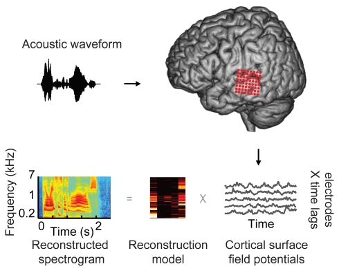
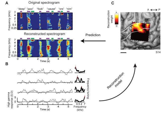
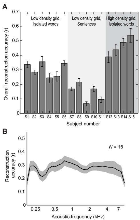
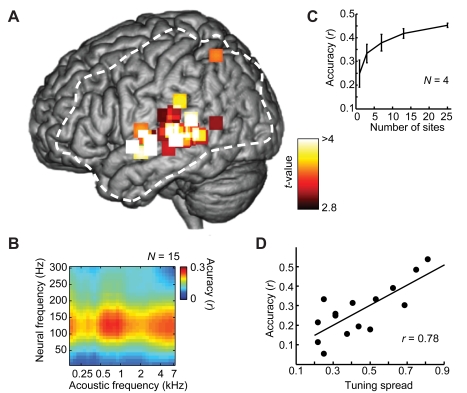
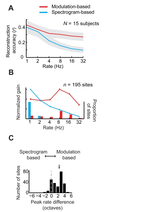
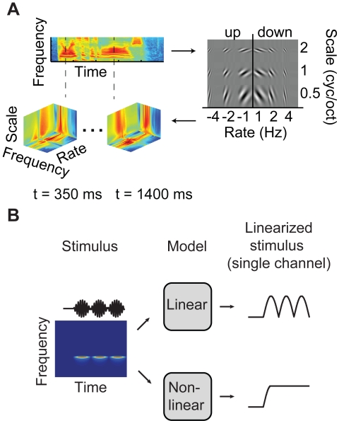
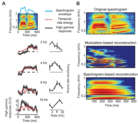
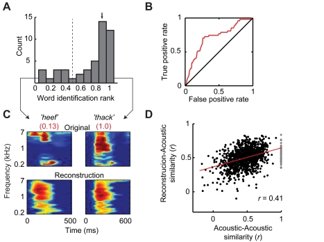
How the human auditory system extracts perceptually relevant acoustic features of speech is unknown. To address this question, we used intracranial recordings from nonprimary auditory cortex in the human superior temporal gyrus to determine what acoustic information in speech sounds can be reconstructed from population neural activity. We found that slow and intermediate temporal fluctuations, such as those corresponding to syllable rate, were accurately reconstructed using a linear model based on the auditory spectrogram. However, reconstruction of fast temporal fluctuations, such as syllable onsets and offsets, required a nonlinear sound representation based on temporal modulation energy. Reconstruction accuracy was highest within the range of spectro-temporal fluctuations that have been found to be critical for speech intelligibility. The decoded speech representations allowed readout and identification of individual words directly from brain activity during single trial sound presentations. These findings reveal neural encoding mechanisms of speech acoustic parameters in higher order human auditory cortex.
Overview
The claims and statistics of this paper haven’t been checked yet.
Free: it reads the open-access text and checks the first 5 claims that cite a source we can check. Create a free account to check every claim.
Integrity signals
Registry
Cites
Statistics
Figures
Verification
Claims the paper makes
The claims and statistics of this paper haven’t been checked yet.
Free: it reads the open-access text and checks the first 5 claims that cite a source we can check. Create a free account to check every claim.
Claims other papers make about this one
Each is checked against this paper’s own text: does it say what the citing paper says it does?
The cited source says what the claim attributes to it.
In the citing paper
“Neural activity in the STG encodes acoustic features — for example, recurring speech sound patterns in the mel-spectrogram — during speech perception53,54 and may be used to reconstruct perceived speech55,56.”
From The speech neuroprosthesis (2024) · cites this paper as [56]
Self-check
Percentages, sums and reported differences re-computed from the paper’s own numbers.
The self-check needs the paper’s full text.
Citations
Cites
The Elements of Statistical Learning
Hastie, T., Tibshirani, R., & Friedman, J. (2009) · Springer Series in Statistics · doi:10.1007/978-0-387-84858-7 · Cited by 25,970
Receptive fields, binocular interaction and functional architecture in the cat’s visual cortex
Hubel, D. H., & Wiesel, T. N. (1962) · The Journal of Physiology · doi:10.1113/jphysiol.1962.sp006837 · Cited by 13,680 · cited 1×
“The modulation model therefore represents an auditory analog to the classical energy model of complex cells in the visual system [32–36], which are invariant to the spatial phase of visual stimuli.”
MethodFundamentals of speech recognition
Rabiner, L. R., & Juang, B.-H. F. (1993) · Cited by 7,680
The cortical organization of speech processing
Hickok, G., & Poeppel, D. (2007) · Nature Reviews Neuroscience · doi:10.1038/nrn2113 · Cited by 5,495 · cited 2×
“For speech comprehension, it is hypothesized that intermediate and higher-order auditory areas extract or construct information-rich features of speech, while discarding nonessential low-level acoustic information [4,5,9, 10,43].”
BackgroundSpatiotemporal energy models for the perception of motion
Adelson, E. H., & Bergen, J. R. (1985) · Journal of the Optical Society of America A · doi:10.1364/josaa.2.000284 · Cited by 3,442 · cited 2×
“Such amplitude-based coding schemes are broadly referred to as ‘‘energy models’’ [32,33].”
BackgroundDISCONNEXION SYNDROMES IN ANIMALS AND MAN
GESCHWIND, N. (1965) · Brain · doi:10.1093/brain/88.2.237 · Cited by 3,403 · cited 5×
“To recover the acoustic waveform from the spectrogram, we used an iterative projection algorithm to estimate the phase [8].”
BackgroundMethodInfluentialTIMIT Acoustic-Phonetic Continuous Speech Corpus
Garofolo, J. S., Lamel, L. F., Fisher, W. M., Pallett, D. S., Dahlgren, N. L., Zue, V. W., & Fiscus, J. G. (2020) · Americanae (AECID Library) · doi:10.35111/17gk-bn40 · Cited by 2,508
Maps and streams in the auditory cortex: nonhuman primates illuminate human speech processing
Rauschecker, J. P., & Scott, S. K. (2009) · Nature Neuroscience · doi:10.1038/nn.2331 · Cited by 1,766 · cited 5×
“Beyond primary auditory areas, further processing in intermediate and higher-order auditory cortex likely results in additional stimulus transformations [5].”
BackgroundResultInfluentialLogothetis, N. K., & Wandell, B. A. (2004) · Annual Review of Physiology · doi:10.1146/annurev.physiol.66.082602.092845 · Cited by 1,568 · cited 1×
“This is consistent with robust speech-induced high gamma responses reported in previous intracranial studies [24–29] and with observed correlations between high gamma power and local spike rate [30].”
ResultIdentifying natural images from human brain activity
Kay, K. N., Naselaris, T., Prenger, R. J., & Gallant, J. L. (2008) · Nature · doi:10.1038/nature06713 · Cited by 1,286 · cited 2×
“An important application of this approach has also been demonstrated in the study of visual object recognition in the primate visual system [36,49,50].”
BackgroundMethod
Cited by
Cortical tracking of hierarchical linguistic structures in connected speech
Ding, N., Melloni, L., Zhang, H., Tian, X., & Poeppel, D. (2016) · Nature Neuroscience · doi:10.1038/nn.4186 · Cited by 1,059
Selective cortical representation of attended speaker in multi-talker speech perception
Mesgarani, N., & Chang, E. F. (2012) · Nature · doi:10.1038/nature11020 · Cited by 1,007
Self-citationMechanisms underlying selective neuronal tracking of attended speech at a “cocktail party”
Zion Golumbic, E. M., Ding, N., Bickel, S., Lakatos, P., Schevon, C. A., McKhann, G. M., Goodman, R. R., Emerson, R., Mehta, A. D., Simon, J. Z., et al. (2013) · Neuron · doi:10.1016/j.neuron.2012.12.037 · Cited by 909
“This selectivity itself seems to sharpen as a sentence unfolds.”
BackgroundInfluentialSpeech synthesis from neural decoding of spoken sentences
Anumanchipalli, G. K., Chartier, J., & Chang, E. F. (2019) · Nature · doi:10.1038/s41586-019-1119-1 · Cited by 883
“Meanwhile, decoding of auditory cortex responses has been more successful for speech sounds 30,31 in part because of the direct relationship between the auditory encoding of spectrotemporal information and the reconstructed spectrogram.”
BackgroundSelf-citationEmergence of neural encoding of auditory objects while listening to competing speakers
Ding, N., & Simon, J. Z. (2012) · Proceedings of the National Academy of Sciences · doi:10.1073/pnas.1205381109 · Cited by 835
“These hypothesized, object-specific neural representations are investigated and revealed, using single-trial neural recordings and an advanced neural decoding method that parallels state-of-theart analysis methods used in functional MRI (fMRI) (23) and intracranial recording (24, 25).”
MethodAttentional Selection in a Cocktail Party Environment Can Be Decoded from Single-Trial EEG
O'Sullivan, J. A., Power, A. J., Mesgarani, N., Rajaram, S., Foxe, J. J., Shinn-Cunningham, B. G., Slaney, M., Shamma, S. A., & Lalor, E. C. (2015) · Cerebral Cortex · doi:10.1093/cercor/bht355 · Cited by 824
“…studies have used recorded cortical population data to estimate the input stimulus using a mapping approach in the reverse direction (i.e., from the neural data back to the stimulus) (Rieke et al. 1995; Stanley et al. 1999; Mesgarani et al. 2009; Pasley et al. 2012; Zion Golumbic et al. 2013).”
BackgroundMethodInfluentialSelf-citationDecoding Neural Representational Spaces Using Multivariate Pattern Analysis
Haxby, J. V., Connolly, A. C., & Guntupalli, J. S. (2014) · Annual Review of Neuroscience · doi:10.1146/annurev-neuro-062012-170325 · Cited by 717
“A study of brain activity that closely resembled the original words (Pasley et al. 2012).”
BackgroundCrosse, M. J., Di Liberto, G. M., Bednar, A., & Lalor, E. C. (2016) · Frontiers in Human Neuroscience · doi:10.3389/fnhum.2016.00604 · Cited by 705
“…inclusion of all response channels in the backward model is advantageous because the reconstruction method gives a low weighting to irrelevant channels whilst allowing the model to capture additional variance using channels potentially excluded by feature selection approaches (Pasley et al., 2012).”
BackgroundMethodSpeech rhythms and multiplexed oscillatory sensory coding in the human brain
Gross, J., Hoogenboom, N., Thut, G., Schyns, P., Panzeri, S., Belin, P., & Garrod, S. (2013) · PLoS Biology · doi:10.1371/journal.pbio.1001752 · Cited by 643
Promises and limitations of human intracranial electroencephalography
Parvizi, J., & Kastner, S. (2018) · Nature Neuroscience · doi:10.1038/s41593-018-0108-2 · Cited by 631
Low-Frequency Cortical Entrainment to Speech Reflects Phoneme-Level Processing
Di Liberto, G. M., O’Sullivan, J. A., & Lalor, E. C. (2015) · Current Biology · doi:10.1016/j.cub.2015.08.030 · Cited by 578
“Robust mappings between speech spectrograms and high-gamma-frequency ECoG have been previously shown [24].”
BackgroundNeural Cross-Frequency Coupling: Connecting Architectures, Mechanisms, and Functions
Hyafil, A., Giraud, A.-L., Fontolan, L., & Gutkin, B. (2015) · Trends in Neurosciences · doi:10.1016/j.tins.2015.09.001 · Cited by 509
“While slow oscillations in sensory areas re fl ect the rhythm of the sensory signal or of sensory sampling, fast gamma oscillations underpin fi ne-grained sensory processing in a bottom-up fashion [28,39,74,83].”
Lachaux, J.-P., Axmacher, N., Mormann, F., Halgren, E., & Crone, N. E. (2012) · Progress in Neurobiology · doi:10.1016/j.pneurobio.2012.06.008 · Cited by 506
“…useful index of cortical activation with a temporal precision adequate, in most cases, to contrast and compare the time courses of cortical activations in the various language areas (Canolty et al., 2007; Crone et al., 2001b; Edwards et al., 2010; Pei et al., 2011; Pasley et al., 2012).”
BackgroundSelf-citationMaterials for flexible bioelectronic systems as chronic neural interfaces
Song, E., Li, J., Won, S. M., Bai, W., & Rogers, J. A. (2020) · Nature Materials · doi:10.1038/s41563-020-0679-7 · Cited by 498
Cortical entrainment to continuous speech: functional roles and interpretations
Ding, N., & Simon, J. Z. (2014) · Frontiers in Human Neuroscience · doi:10.3389/fnhum.2014.00311 · Cited by 443
“REVIEW ARTICLE published: 28 May 2014 doi: 10.3389/fnhum.2014.00311 Cortical entrainment to continuous speech: functional roles and interpretations”
BackgroundInfluentialSemantic reconstruction of continuous language from non-invasive brain recordings
Tang, J., LeBel, A., Jain, S., & Huth, A. G. (2023) · Nature Neuroscience · doi:10.1038/s41593-023-01304-9 · Cited by 442
“In contrast, our decoder represents language using semantic features and primarily uses data from regions that encode semantic representations 5 during language perception 2 .”
MethodA Minimally Invasive 64-Channel Wireless μECoG Implant
Muller, R., Le, H.-P., Li, W., Ledochowitsch, P., Gambini, S., Bjorninen, T., Koralek, A., Carmena, J. M., Maharbiz, M. M., Alon, E., et al. (2015) · IEEE Journal of Solid-State Circuits · doi:10.1109/jssc.2014.2364824 · Cited by 372
“I N ORDER to realize the vision of fully autonomous brain–machine interface (BMI) systems, neural implant devices must not only be effective in their function, but should also meet clinical constraints such as ease of implantation, longevity, safety, and small size.”
BackgroundInfluentialThe Cortical Organization of Syntax
Matchin, W., & Hickok, G. (2020) · Cerebral Cortex · doi:10.1093/cercor/bhz180 · Cited by 370
Buzsáki, G. (2019) · doi:10.1093/oso/9780190905385.001.0001 · Cited by 358
Rhythmic facilitation of sensory processing: A critical review
Haegens, S., & Zion Golumbic, E. (2018) · Neuroscience & Biobehavioral Reviews · doi:10.1016/j.neubiorev.2017.12.002 · Cited by 343
“, 2014), and phonetic features tracked by higher beta/gamma frequencies (Cogan and Poeppel, 2011; Pasley et al., 2012; Gross et al., 2013; Martin et al., 2016).”
BackgroundInfluentialCentral Gain Restores Auditory Processing following Near-Complete Cochlear Denervation
Chambers, A. R., Resnik, J., Yuan, Y., Whitton, J. P., Edge, A. S., Liberman, M. C., & Polley, D. B. (2016) · Neuron · doi:10.1016/j.neuron.2015.12.041 · Cited by 302
“High-fidelity sound representations at early stages of auditory processing are reformatted as abstractions of the source signal in higher centers (Atencio et al., 2012; Pasley et al., 2012; Rabinowitz et al., 2013; Wang et al., 2008).”
Brain-to-text: decoding spoken phrases from phone representations in the brain
Herff, C., Heger, D., de Pesters, A., Telaar, D., Brunner, P., Schalk, G., & Schultz, T. (2015) · Frontiers in Neuroscience · doi:10.3389/fnins.2015.00217 · Cited by 297
Speech Intelligibility Predicted from Neural Entrainment of the Speech Envelope
Vanthornhout, J., Decruy, L. P., Wouters, J. M., Simon, J. Z., & Francart, T. (2018) · Journal of the Association for Research in Otolaryngology · doi:10.1007/s10162-018-0654-z · Cited by 290
Neural processing of natural sounds
Theunissen, F. E., & Elie, J. E. (2014) · Nature Reviews Neuroscience · doi:10.1038/nrn3731 · Cited by 240
“Second, advances in both invasive [133,134] and non-invasive [135] neurophysiological recordings in humans will further allow researchers to make links between animal work and human work.”
BackgroundSantoro, R., Moerel, M., De Martino, F., Goebel, R., Ugurbil, K., Yacoub, E., & Formisano, E. (2014) · PLoS Computational Biology · doi:10.1371/journal.pcbi.1003412 · Cited by 240
“The encoding mechanism that our results support is consistent with a recent study showing that a frequency-specific representation of combined spectro-temporal modulations allows the accurate reconstruction of speech in the human posterior superior temporal gyrus [31].”
ResultNoise-robust cortical tracking of attended speech in real-world acoustic scenes
Fuglsang, S. A., Dau, T., & Hjortkjær, J. (2017) · NeuroImage · doi:10.1016/j.neuroimage.2017.04.026 · Cited by 236
Speech encoding by coupled cortical theta and gamma oscillations
Hyafil, A., Fontolan, L., Kabdebon, C., Gutkin, B., & Giraud, A.-L. (2015) · eLife · doi:10.7554/elife.06213 · Cited by 235
“Unlike the classical 50–80 Hz PING seen in in vitro preparations of rat auditory cortex (Ainsworth et al., 2011), our network produced a lower gamma frequency around 30 Hz, as observed in human auditory cortex in response to speech (Nourski et al., 2009; Pasley et al., 2012).”
BackgroundMirkovic, B., Debener, S., Jaeger, M., & De Vos, M. (2015) · Journal of Neural Engineering · doi:10.1088/1741-2560/12/4/046007 · Cited by 231
“Single-trial intracranial recordings from the auditory cortex were utilized for the purpose of explaining neural encoding mechanisms (Pasley et al 2012).”
MethodAdvances in human intracranial electroencephalography research, guidelines and good practices
Mercier, M. R., Dubarry, A.-S., Tadel, F., Avanzini, P., Axmacher, N., Cellier, D., Vecchio, M. D., Hamilton, L. S., Hermes, D., Kahana, M. J., et al. (2022) · NeuroImage · doi:10.1016/j.neuroimage.2022.119438 · Cited by 229
Self-citationNeural population coding: combining insights from microscopic and mass signals
Panzeri, S., Macke, J. H., Gross, J., & Kayser, C. (2015) · Trends in Cognitive Sciences · doi:10.1016/j.tics.2015.01.002 · Cited by 226
Speech synthesis from ECoG using densely connected 3D convolutional neural networks
Angrick, M., Herff, C., Mugler, E., Tate, M. C., Slutzky, M. W., Krusienski, D. J., & Schultz, T. (2019) · Journal of Neural Engineering · doi:10.1088/1741-2552/ab0c59 · Cited by 225
“We discarded the phase information and only used the magnitude of the spectrograms [29, 52, 28].”
BackgroundMethodReal-time decoding of question-and-answer speech dialogue using human cortical activity
Moses, D. A., Leonard, M. K., Makin, J. G., & Chang, E. F. (2019) · Nature Communications · doi:10.1038/s41467-019-10994-4 · Cited by 224
Self-citationTowards reconstructing intelligible speech from the human auditory cortex
Akbari, H., Khalighinejad, B., Herrero, J. L., Mehta, A. D., & Mesgarani, N. (2019) · Scientific Reports · doi:10.1038/s41598-018-37359-z · Cited by 221
Self-citationMoerel, M., De Martino, F., & Formisano, E. (2012) · The Journal of Neuroscience · doi:10.1523/jneurosci.1388-12.2012 · Cited by 219
Decoding speech perception from non-invasive brain recordings
Défossez, A., Caucheteux, C., Rapin, J., Kabeli, O., & King, J.-R. (2023) · Nature Machine Intelligence · doi:10.1038/s42256-023-00714-5 · Cited by 215
“To tackle this issue, previous studies have primarily used supervised models targeting well-defined features of language, such as individual letters, phonemes, or frequency bands of the audio spectrogram [5, 24, 44, 46, 57, 64, 70, 74, 76, 93].”
Method(2013) · Handbook of Clinical Neurology · doi:10.1016/b978-0-444-52901-5.00006-x · Cited by 212
Crosse, M. J., Butler, J. S., & Lalor, E. C. (2015) · The Journal of Neuroscience · doi:10.1523/jneurosci.1829-15.2015 · Cited by 208
“Our decision to include all 128 channels of EEG in the reconstruction analysis is justified because irrelevant filter channels can maintain zero weight while allowing the model to capture additional variance (Pasley et al., 2012).”
BackgroundBiosignal-Based Spoken Communication: A Survey
Schultz, T., Wand, M., Hueber, T., Krusienski, D. J., Herff, C., & Brumberg, J. S. (2017) · IEEE/ACM Transactions on Audio, Speech, and Language Processing · doi:10.1109/taslp.2017.2752365 · Cited by 201
“tening [127].”
Decoding spectrotemporal features of overt and covert speech from the human cortex
Martin, S., Brunner, P., Holdgraf, C., Heinze, H.-J., Crone, N. E., Rieger, J., Schalk, G., Knight, R. T., & Pasley, B. N. (2014) · Frontiers in Neuroengineering · doi:10.3389/fneng.2014.00014 · Cited by 200
Self-citationDecoding the auditory brain with canonical component analysis
de Cheveigné, A., Wong, D. D. E., Di Liberto, G. M., Hjortkjær, J., Slaney, M., & Lalor, E. (2018) · NeuroImage · doi:10.1016/j.neuroimage.2018.01.033 · Cited by 198
“This study builds upon a growing body of work exploring stimulusresponse relations using system-identification techniques and decoding (Lalor et al., 2009; Lalor and Foxe, 2010; Power et al., 2011, 2012; Pasley et al., 2012; Ding and Simon, 2012; Brandmeyer et al., 2013; Ding and Simon, 2013; Ding et al., 2014; O'Sull…”
Compensatory changes in cortical resource allocation in adults with hearing loss
Campbell, J., & Sharma, A. (2013) · Frontiers in Systems Neuroscience · doi:10.3389/fnsys.2013.00071 · Cited by 198
Discrete Neocortical Dynamics Predict Behavioral Categorization of Sounds
Bathellier, B., Ushakova, L., & Rumpel, S. (2012) · Neuron · doi:10.1016/j.neuron.2012.07.008 · Cited by 194
“This is in line with the observation that arrays of local field potential recordings in the human brain are sufficient to retrieve much of the information about sounds despite their lack of spatial precision and their inability to account for single-neuron activity (Pasley et al., 2012).”
Spectrotemporal modulation provides a unifying framework for auditory cortical asymmetries
Flinker, A., Doyle, W. K., Mehta, A. D., Devinsky, O., & Poeppel, D. (2019) · Nature Human Behaviour · doi:10.1038/s41562-019-0548-z · Cited by 194
Self-citationA Precluding But Not Ensuring Role of Entrained Low-Frequency Oscillations for Auditory Perception
Ng, B. S. W., Schroeder, T., & Kayser, C. (2012) · The Journal of Neuroscience · doi:10.1523/jneurosci.1877-12.2012 · Cited by 187
“Slow delta and theta oscillations entrain to sound se- quences or speech, as evidenced by studies on humans (Luo and Poeppel, 2007; Howard and Poeppel, 2010; Ng et al., 2012; Pasley et al., 2012) or animals (Lakatos et al., 2008; Kayser et al., 2009).”
BackgroundEEG-based detection of the locus of auditory attention with convolutional neural networks
Vandecappelle, S., Deckers, L., Das, N., Ansari, A. H., Bertrand, A., & Francart, T. (2021) · eLife · doi:10.7554/elife.56481 · Cited by 187
“A common approach is stimulus reconstruction, where the post-stimulus brain activity is used to decode and reconstruct the attended stimulus envelope (O’sullivan et al., 2014; Pasley et al., 2012).”
Tracing the emergence of categorical speech perception in the human auditory system
Bidelman, G. M., Moreno, S., & Alain, C. (2013) · NeuroImage · doi:10.1016/j.neuroimage.2013.04.093 · Cited by 186
“…modulations in electrical brain activity in response to salient features of speech necessary for its comprehension including voice-onset time (Sharma and Dorman, 1999), spectrotemporal modulations (Pasley et al., 2012), voice pitch (Zhang et al., 2012), and timbre cues (Agung et al., 2006).”
Classifying phonological categories in imagined and articulated speech
Zhao, S., & Rudzicz, F. (2015) · 2015 IEEE International Conference on Acoustics, Speech and Signal Processing (ICASSP) · doi:10.1109/icassp.2015.7178118 · Cited by 182
“’s work with invasive methods [4], potentially towards mapping imagined speech to synthetic speech.”
BackgroundMethodA Spatial Map of Onset and Sustained Responses to Speech in the Human Superior Temporal Gyrus
Hamilton, L. S., Edwards, E., & Chang, E. F. (2018) · Current Biology · doi:10.1016/j.cub.2018.04.033 · Cited by 180
“In agreement with previous work [12, 13, 21, 26], we found higher temporal and lower spectral modulation selectivity in caudal onset electrodes, whereas rostral sustained electrodes showed low temporal/high spectral modulation selectivity (Figure 2D).”
Self-citationEncoding and Decoding Models in Cognitive Electrophysiology
Holdgraf, C., Rieger, J. W., Micheli, C., Martin, S., Knight, R. T., & Theunissen, F. E. (2017) · Frontiers in Systems Neuroscience · doi:10.3389/fnsys.2017.00061 · Cited by 181
“…features of the sound spectrum, such as formant frequencies (Brumberg et al., 2010), amplitude power, and spectrotemporal modulations (Pasley et al., 2012; Martin et al., 2014, 2016), melfrequency cepstral-coefficients (Chakrabarti et al., 2013), or the speech envelope (Kubanek et…”
BackgroundMethodInfluentialSelf-citationLiberto, G. M. D., Peter, V., Kalashnikova, M., Goswami, U., Burnham, D. K., & Lalor, E. C. (2018) · NeuroImage · doi:10.1016/j.neuroimage.2018.03.072 · Cited by 176
Target Speaker Detection with Concealed EEG Around the Ear
Mirkovic, B., Bleichner, M. G., Vos, M. D., & Debener, S. (2016) · Frontiers in Neuroscience · doi:10.3389/fnins.2016.00349 · Cited by 175
“The procedure of choice for detecting the target speaker has been the envelope tracking algorithm (Pasley et al., 2012; O’Sullivan et al., 2014; Crosse et al., 2015; Mirkovic et al., 2015) which relates the envelope of speech to the neural signal.”
MethodSimple Acoustic Features Can Explain Phoneme-Based Predictions of Cortical Responses to Speech
Daube, C., Ince, R. A. A., & Groß, J. (2019) · Current Biology · doi:10.1016/j.cub.2019.04.067 · Cited by 176
Word pair classification during imagined speech using direct brain recordings
Martin, S., Brunner, P., Iturrate, I., Millán, J. D. R., Schalk, G., Knight, R. T., & Pasley, B. N. (2016) · Scientific Reports · doi:10.1038/srep25803 · Cited by 171
“Because high gamma neural activity is known to track the speech envelope 22,23,27,33 , we assumed that temporal variations in overt and imagined speech would also be represented by the measured neural responses.”
BackgroundSelf-citationSuppression of competing speech through entrainment of cortical oscillations
Horton, C., D'Zmura, M., & Srinivasan, R. (2013) · Journal of Neurophysiology · doi:10.1152/jn.01026.2012 · Cited by 167
Wong, D. D. E., Fuglsang, S. A., Hjortkjær, J., Ceolini, E., Slaney, M., & de Cheveigné, A. (2018) · Frontiers in Neuroscience · doi:10.3389/fnins.2018.00531 · Cited by 171
“It is likely that other neural frequency bands robustly track attended speech (e.g., high gamma power Pasley et al., 2012) and that the neural decoders potentially could benefit from having access to other neural frequency bands.”
BackgroundConstructing Noise-Invariant Representations of Sound in the Auditory Pathway
Rabinowitz, N. C., Willmore, B. D. B., King, A. J., & Schnupp, J. W. H. (2013) · PLoS Biology · doi:10.1371/journal.pbio.1001710 · Cited by 167
“Population Representations of Sound Given that m- and s-adaptation increase along the auditory pathway, how does this affect the representation of complex sounds by populations of auditory neurons? To answer this, we used a stimulus reconstruction method [42–45] that quantified how accurately the spectrogram of a pres…”
BackgroundMethodHe, B., Yuan, H., Meng, J., & Gao, S. (2020) · Springer eBooks · doi:10.1007/978-3-030-43395-6_4 · Cited by 167
Cross-Modal Re-Organization in Adults with Early Stage Hearing Loss
Campbell, J., & Sharma, A. (2014) · PLoS ONE · doi:10.1371/journal.pone.0090594 · Cited by 166
Large-scale single-neuron speech sound encoding across the depth of human cortex
Leonard, M. K., Gwilliams, L., Sellers, K. K., Chung, J. E., Xu, D., Mischler, G., Mesgarani, N., Welkenhuysen, M., Dutta, B., & Chang, E. F. (2024) · Nature · doi:10.1038/s41586-023-06839-2 · Cited by 163
“Performance was quantified using Pearson correlation between the predicted time course and the true time course for each frequency and then averaged across the 80 frequency bands 68 .”
Self-citationRiès, S., Dronkers, N. F., & Knight, R. T. (2016) · Annals of the New York Academy of Sciences · doi:10.1111/nyas.12993 · Cited by 163
Self-citationEyndhoven, S. V., Francart, T., & Bertrand, A. (2016) · IEEE Transactions on Biomedical Engineering · doi:10.1109/tbme.2016.2587382 · Cited by 162
“Earlier studies showed that the low-frequency variations of speech envelopes (between approximately 1 and 9 Hz) are encoded in the evoked brain activity [20], [21], and that this mapping differs whether the speech is attended to by the subject (or not) in a multispeaker environment [6]–[8], [22], [23].”
Neuroimaging-based biomarkers for pain: state of the field and current directions
van der Miesen, M. M., Lindquist, M. A., & Wager, T. D. (2019) · PAIN Reports · doi:10.1097/pr9.0000000000000751 · Cited by 161
“For example, a visual stimulus might be decomposed into a set of features using Gabor filters,(62) words into semantic features,(93) and speech into acoustic features.(103) The voxel’s activity is regressed on these”
MethodHullett, P. W., Hamilton, L. S., Mesgarani, N., Schreiner, C. E., & Chang, E. F. (2016) · The Journal of Neuroscience · doi:10.1523/jneurosci.1779-15.2016 · Cited by 160
“…average best temporal modulation: 2– 8 Hz; Binder et al., 1994; Tanaka et al., 2000; Harms and Melcher, 2002; Langers et al., 2003; Liégeois-Chauvel et al., 2004; Rinne et al., 2005; Schönwiesner and Zatorre, 2009; Overath et al., 2012; Pasley et al., 2012; Wang et al., 2012; Gross et al., 2013).”
BackgroundSelf-citationSpeech-Specific Tuning of Neurons in Human Superior Temporal Gyrus
Chan, A. M., Dykstra, A. R., Jayaram, V., Leonard, M. K., Travis, K. E., Gygi, B., Baker, J. M., Eskandar, E. N., Hochberg, L. R., Halgren, E., et al. (2013) · Cerebral Cortex · doi:10.1093/cercor/bht127 · Cited by 152
Delta- and theta-band cortical tracking and phase-amplitude coupling to sung speech by infants
Attaheri, A., Choisdealbha, Á. N., Liberto, G. M. D., Rocha, S., Brusini, P., Mead, N., Olawole‐Scott, H., Boutris, P., Gibbon, S., Williams, I., et al. (2021) · NeuroImage · doi:10.1016/j.neuroimage.2021.118698 · Cited by 152
Thinking out loud, an open-access EEG-based BCI dataset for inner speech recognition
Nieto, N., Peterson, V., Rufiner, H. L., Kamienkowski, J. E., & Spies, R. D. (2022) · Scientific Data · doi:10.1038/s41597-022-01147-2 · Cited by 153
Generative Adversarial Networks Conditioned by Brain Signals
Palazzo, S., Spampinato, C., Kavasidis, I., Giordano, D., & Shah, M. A. (2017) · IEEE/CVF International Conference on Computer Vision (ICCV) · doi:10.1109/iccv.2017.369 · Cited by 150
“In [20], the authors describe an approach to recreate (partially) speech stimuli based on human auditory cortex data, acquired by cortical surface electrode arrays.”
BackgroundDistinct contributions of low- and high-frequency neural oscillations to speech comprehension
Kösem, A., & van Wassenhove, V. (2016) · Language Cognition and Neuroscience · doi:10.1080/23273798.2016.1238495 · Cited by 149
“First, the content of heard and attended speech signals can be decoded from high-frequency power (Mesgarani & Chang, 2012; Pasley et al., 2012; Zion Golumbic et al., 2013).”
BackgroundInfluentialCortical gamma oscillations: the functional key is activation, not cognition
Merker, B. H. (2013) · Neuroscience & Biobehavioral Reviews · doi:10.1016/j.neubiorev.2013.01.013 · Cited by 146
Reconstructing the spectrotemporal modulations of real-life sounds from fMRI response patterns
Santoro, R., Moerel, M., Martino, F. D., Valente, G., Uǧurbil, K., Yacoub, E. S., & Formisano, E. (2017) · Proceedings of the National Academy of Sciences · doi:10.1073/pnas.1617622114 · Cited by 143
“Although consistent with recent reports of speech spectrogram reconstruction from ECoG recordings (12), this result is surprising, given the low temporal resolution of fMRI and the coarse temporal sampling [repetition time (TR) = 2.”
BackgroundResultLeong, V., & Goswami, U. (2013) · Hearing Research · doi:10.1016/j.heares.2013.07.015 · Cited by 140
“Recent advances in methods that use participants’ neural entrained responses to ‘reconstruct’ the speech envelope (thereby visualising phonological encoding in the brain) provide one means to investigate such representational integrity (Pasley et al., 2012; Ding and Simon, 2012).”
Automatic Speech Recognition from Neural Signals: A Focused Review
Herff, C., & Schultz, T. (2016) · Frontiers in Neuroscience · doi:10.3389/fnins.2016.00429 · Cited by 138
“Pasley et al. (2012) have shown that perceived speech could be reconstructed from ECoG recordings.”
BackgroundAnatomic organization of the auditory cortex
Hackett, T. A. (2015) · Handbook of clinical neurology · doi:10.1016/b978-0-444-62630-1.00002-0 · Cited by 131
Translating the Brain-Machine Interface
Thakor, N. V. (2013) · Science Translational Medicine · doi:10.1126/scitranslmed.3007303 · Cited by 128
“Beyond these, more developed applications, such as prostheses that restore speech ( 28 – 30 ) or memory ( 73 ), are also being investigated, although these research projects are in early stages of feasibility testing and demonstration.”
BackgroundAhn, S., Cho, H., Kwon, M., Kim, K., Kwon, H., Kim, B. S., Chang, W. S., Chang, J. W., & Jun, S. C. (2017) · Human Brain Mapping · doi:10.1002/hbm.23834 · Cited by 129
“Further, neurophysiological evidence of gamma band function has been found in MEG [Basirat et al., 2008; Kaiser et al., 2003; Kingyon et al., 2015; Palva et al., 2002] and ECoG studies [Crone et al., 2001a,b; Pasley et al., 2012; Potes et al., 2014; Towle et al., 2008].”
BackgroundDas, N., Bertrand, A., & Francart, T. (2018) · Journal of Neural Engineering · doi:10.1088/1741-2552/aae0a6 · Cited by 110
“This choice of the frequency range was based on earlier studies (Das et al., 2016; Ding and Simon, 2012b; Golumbic et al., 2013; Pasley et al., 2012) that showed the best attention decoding performance based on cortical envelope tracking in this range.”
BackgroundMethodAngrick, M., Ottenhoff, M. C., Diener, L., Ivucic, D., Ivucic, G., Goulis, S., Saal, J., Colon, A. J., Wagner, L., Krusienski, D. J., et al. (2021) · Communications Biology · doi:10.1038/s42003-021-02578-0 · Cited by 125
Friston, K. J., Sajid, N., Quiroga‐Martinez, D. R., Parr, T., Price, C. J., & Holmes, E. (2020) · Hearing Research · doi:10.1016/j.heares.2020.107998 · Cited by 129
Decoding spoken phonemes from sensorimotor cortex with high-density ECoG grids
Ramsey, N. F., Salari, E., Aarnoutse, E. J., Vansteensel, M. J., Bleichner, M. G., & Freudenburg, Z. V. (2018) · NeuroImage · doi:10.1016/j.neuroimage.2017.10.011 · Cited by 124
“Decoding perceived speech has been shown by several groups to be feasible from auditory cortex, which in itself contributes to understanding how the auditory cortex is organized (Formisano et al., 2008; Mesgarani et al., 2014; Pasley et al., 2012).”
How Movement Modulates Hearing
Schneider, D. M., & MOONEY, R. D. (2018) · Annual Review of Neuroscience · doi:10.1146/annurev-neuro-072116-031215 · Cited by 125
“…patient’s own speech suppresses many auditory cortical neurons relative to speech playback, while revealing a smaller number of sites (or neurons) either equally excited during both conditions or more excited during vocalization (Creutzfeldt et al. 1989, Flinker et al. 2010, Pasley et al. 2012).”
BackgroundThe myth of categorical perception
McMurray, B. (2022) · The Journal of the Acoustical Society of America · doi:10.1121/10.0016614 · Cited by 126
A Tutorial on Auditory Attention Identification Methods
Aličković, E., Lunner, T., Gustafsson, F., & Ljung, L. (2019) · Frontiers in Neuroscience · doi:10.3389/fnins.2019.00153 · Cited by 123
“…(Obleser and Weisz, 2011; Weisz et al., 2011; Henry et al., 2014) and speech entrainment (Ding and Simon, 2012a,b; Mesgarani and Chang, 2012; Pasley et al., 2012; Mirkovic et al., 2015; O’Sullivan et al., 2015, 2017; Ekin et al., 2016; Biesmans et al., 2017; Fuglsang et al., 2017; Kaya and…”
BackgroundPefkou, M., Arnal, L. H., Fontolan, L., & Giraud, A. (2017) · Journal of Neuroscience · doi:10.1523/jneurosci.2882-16.2017 · Cited by 120
Predicting BCI Subject Performance Using Probabilistic Spatio-Temporal Filters
Suk, H., Fazli, S., Mehnert, J., Müller, K., & Lee, S. (2014) · PLoS ONE · doi:10.1371/journal.pone.0087056 · Cited by 119
“, motor movement [32,33] or auditory processing [34].”
BackgroundHerff, C., Diener, L., Angrick, M., Mugler, E., Tate, M. C., Goldrick, M. A., Krusienski, D. J., Slutzky, M. W., & Schultz, T. (2019) · Frontiers in Neuroscience · doi:10.3389/fnins.2019.01267 · Cited by 118
“However, we reconstructed articulated speech from motor areas, while Pasley et al. (2012) employed activity in auditory areas during speech perception for their approach.”
BackgroundMethodResultParthasarathy, A., Hancock, K. E., Bennett, K. K., DeGruttola, V. G., & Polley, D. B. (2020) · eLife · doi:10.7554/elife.51419 · Cited by 118
“, 2013) or direct neural speech decoding (Ding and Simon, 2012; Ding and Simon, 2009; Maddox and Lee, 2018; Mesgarani et al., 2014; Mesgarani et al., 2008; Pasley et al., 2012; Presacco et al., 2016) would very likely capture even more of the unexplained variability in multitalker speech intelligibility, though they o…”
BackgroundThe effect of head-related filtering and ear-specific decoding bias on auditory attention detection*
Das, N., Biesmans, W., Bertrand, A., & Francart, T. (2016) · Journal of Neural Engineering · doi:10.1088/1741-2560/13/5/056014 · Cited by 116
Decoding Inner Speech Using Electrocorticography: Progress and Challenges Toward a Speech Prosthesis
Martin, S., Iturrate, I., Millán, J. D. R., Knight, R. T., & Pasley, B. N. (2018) · Frontiers in Neuroscience · doi:10.3389/fnins.2018.00422 · Cited by 115
“This study therefore provided a unique opportunity to apply direct (as opposed to cross-condition) receptive field modeling techniques (Aertsen et al., 1981; Clopton and Backoff, 1991; Theunissen et al., 2000; Chi et al., 2005; Pasley et al., 2012), which describe neural response properties, for example auditory frequ…”
BackgroundSelf-citationFunctional near-infrared spectroscopy for neuroimaging in cochlear implant recipients
Saliba, J., Bortfeld, H., Levitin, D. J., & Oghalai, J. S. (2016) · Hearing Research · doi:10.1016/j.heares.2016.02.005 · Cited by 114
“Because auditory perception occurs within and beyond the auditory cortex, neuroimaging has the potential to provide an additional clinical measure for assessing whether the electrical stimulation of the cochlea by the CI is reaching and stimulating auditory-specific cortical regions of the brain similar to normalheari…”
BackgroundA high-density, high-channel count, multiplexed μECoG array for auditory-cortex recordings
Escabí, M. A., Read, H. L., Viventi, J., Kim, D., Higgins, N. C., Storace, D. A., Liu, A., Gifford, A. M., Burke, J. F., Campisi, M., et al. (2014) · Journal of Neurophysiology · doi:10.1152/jn.00179.2013 · Cited by 111
Norman-Haignere, S., & McDermott, J. H. (2018) · PLoS Biology · doi:10.1371/journal.pbio.2005127 · Cited by 109
“The approach of learning separate weights for the purpose of reconstruction is standard in the sensory encoding/decoding literature [94].”
BackgroundCortical Representations of Speech in a Multitalker Auditory Scene
Puvvada, K. C., & Simon, J. Z. (2017) · Journal of Neuroscience · doi:10.1523/jneurosci.0938-17.2017 · Cited by 108
Degenhart, A. D., Eles, J. R., Dum, R. P., Mischel, J., Smalianchuk, I., Endler, B., Ashmore, R. C., Tyler‐Kabara, E. C., Hatsopoulos, N. G., Wang, W., et al. (2016) · Journal of Neural Engineering · doi:10.1088/1741-2560/13/4/046019 · Cited by 108
Moses, D. A., Mesgarani, N., Leonard, M. K., & Chang, E. F. (2016) · Journal of Neural Engineering · doi:10.1088/1741-2560/13/5/056004 · Cited by 108
“Previous research has shown that high gamma band activity ( 70 – 150 Hz ) correlates strongly with multi-unit fi ring processes in the brain [ 33 ] and is an effective representation of brain activity during speech processing [ 5, 6, 16, 34 ] .”
BackgroundSelf-citationAkram, S., Presacco, A., Simon, J. Z., Shamma, S., & Babadi, B. (2015) · NeuroImage · doi:10.1016/j.neuroimage.2015.09.048 · Cited by 107
“In the case of listening to speech, it has recently been demonstrated that the auditory response manifested in magnetoencephalographic recordings is strongly modulated by the spectrotemporal features of the speech (Ding and Simon, 2012b; Pasley et al., 2012).”
Self-citationRapid tuning shifts in human auditory cortex enhance speech intelligibility
Holdgraf, C., de Heer, W. A., Pasley, B. N., Rieger, J. W., Crone, N. E., Lin, J. J., Knight, R. T., & Theunissen, F. E. (2016) · Nature Communications · doi:10.1038/ncomms13654 · Cited by 107
“5), and (3) be located on the temporal lobe or perisylvian cortex, regions traditionally associated with spectrotemporal auditory processing 31,32,38 .”
Self-citationAdaptation of the human auditory cortex to changing background noise
Khalighinejad, B., Herrero, J. L., Mehta, A. D., & Mesgarani, N. (2019) · Nature Communications · doi:10.1038/s41467-019-10611-4 · Cited by 104
Self-citationGiordano, B. L., Esposito, M., Valente, G., & Formisano, E. (2023) · Nature Neuroscience · doi:10.1038/s41593-023-01285-9 · Cited by 105
“This is consistent with previous findings 6–8 , 46–”
ResultKong, Y.-Y., Mullangi, A., & Ding, N. (2014) · Hearing Research · doi:10.1016/j.heares.2014.07.009 · Cited by 104
“…a single speech stream is presented in a quiet listening environment, the neural responses from the auditory cortex phase lock to the temporal envelope of the speech signal (e.g., Luo and Poeppel, 2007; Aiken and Picton, 2008; Howard and Poeppel, 2010; Lalor and Foxe, 2010; Pasely et al., 2012).”
Dynamic speech representations in the human temporal lobe
Leonard, M. K., & Chang, E. F. (2014) · Trends in Cognitive Sciences · doi:10.1016/j.tics.2014.05.001 · Cited by 104
“We believe it will prove useful to apply decoding methods that have successfully uncovered speech representations in STG [3,4,54] to these aspects of neural activity that reflect the characteristics of words at both sub-lexical and abstract levels.”
Self-citation
Metadata
- Authors
- Pasley, B. N., David, S. V., Mesgarani, N., Flinker, A., Shamma, S. A., Crone, N. E., Knight, R. T., & Chang, E. F.
- Affiliations
- University of California, Berkeley (US)
- University of Maryland, College Park (US)
- University of California, San Francisco (US)
- Johns Hopkins University (US)
- Corresponding author
- Pasley, Brian N.
- ORCID
- Venue
- PLoS Biology
- Publisher
- Public Library of Science (PLoS)
- Published
- 2012-01-31
- Volume
- 10
- Issue
- 1
- Pages
- e1001251
- ISSN
- 1544-9173 (ISSN-L)
- 1545-7885
- PMC
- PMC3269422
- OpenAlex
- W2005066437
- Cited by
- 604
- References
- 61
- Citations by year
- 2026: 21 · 2025: 30 · 2024: 28 · 2023: 35 · 2022: 36 · 2021: 32 · 2020: 51 · 2019: 66 · 2018: 42 · 2017: 53 · 2016: 43 · 2015: 51 · 2014: 42 · 2013: 50 · 2012: 24
- FWCI
- 27.32
- Type
- journal article
- Language
- en
- Open access
- gold
- doi.org
- Locations
- PLoS Biology (publishedVersion, cc-by)
- Europe PMC (PubMed Central) (publishedVersion, cc-by)
- PubMed Central (publishedVersion, cc-by)
- PubMed (publishedVersion)
- DOAJ (DOAJ: Directory of Open Access Journals) (submittedVersion)
- eScholarship (California Digital Library) (submittedVersion)
- Figshare (submittedVersion, cc-by)
- Funders
- National Institutes of Health (2r01ns021135-33, 5r00ns065120-04)
- U.S. Public Health Service (P04813)
- National Institute on Deafness and Other Communication Disorders (K99DC010439, K99DC012804, R01DC012379)
- National Institute of Neurological Disorders and Stroke (NS-40596, NS-21135, K99NS065120, R56NS021135, R37NS021135, R01NS040596, R00-NS065120, R01 NS-021135)
- Topics
- Life Sciences › Neuroscience › Cognitive Neuroscience › Neuroscience and Music Perception
- Social Sciences › Psychology › Experimental and Cognitive Psychology › Phonetics and Phonology Research
- Life Sciences › Neuroscience › Cognitive Neuroscience › Neurobiology of Language and Bilingualism
- Keywords
- speech perception, auditory cortex, superior temporal gyrus, neural decoding, speech reconstruction, acoustic features, syllable rate, word recognition, nonlinear decoding, speech intelligibility
- MeSH terms
- Algorithms, Auditory Cortex, Brain Mapping, Computer Simulation, Electrodes, Implanted, Electroencephalography, Female, Humans, Male, Models, Biological, Speech Acoustics, Linear Models
About these checks
Registry, retraction, Cites and statistics results are computed, not judged, with one exception: a printed reference that no index lists is read once by a model before it counts as a citation error. Claims are extracted by a model and kept only when their quote appears verbatim in the text; each cited source is then checked, with a model’s help, for whether it says what the claim relies on. Those verdicts can be wrong — read the claim’s quote and the cited source before relying on one.
Statistics and arithmetic are recomputed, not judged.
Confidence bands are shown only for fields calibrated on our annotated test set. None is calibrated yet, so no band is shown.
What counts as a claim ›How we measure confidence ›How we check this ›
Are you an author, or do you see a problem with this page? Request a review
Data sources
Bibliographic data: Semantic Scholar, OpenAlex, Crossref.
Contains information from the Semantic Scholar Academic Graph Datasets, made available under the ODC Attribution License (ODC-BY 1.0).
Semantic Scholar’s data is described in: Kinney, R., et al. (2023). The Semantic Scholar Open Data Platform. arXiv:2301.10140.
