

The DOI matches its Crossref record; 125 of the 125 references it cites were found in a registry or an index.
Task-Based Core-Periphery Organization of Human Brain Dynamics
Open accessAbstract
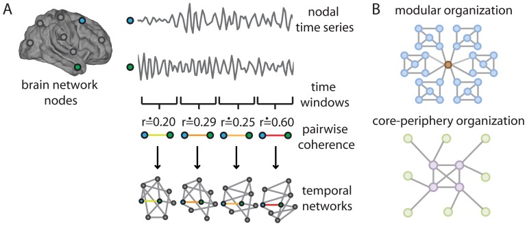
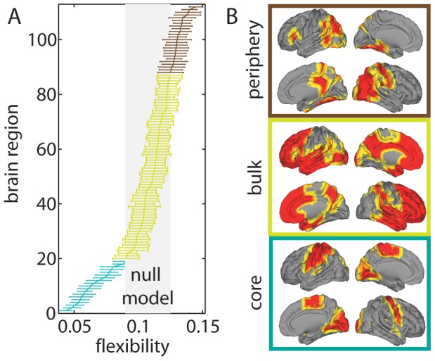
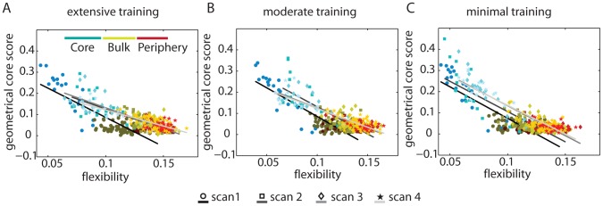
As a person learns a new skill, distinct synapses, brain regions, and circuits are engaged and change over time. In this paper, we develop methods to examine patterns of correlated activity across a large set of brain regions. Our goal is to identify properties that enable robust learning of a motor skill. We measure brain activity during motor sequencing and characterize network properties based on coherent activity between brain regions. Using recently developed algorithms to detect time-evolving communities, we find that the complex reconfiguration patterns of the brain's putative functional modules that control learning can be described parsimoniously by the combined presence of a relatively stiff temporal core that is composed primarily of sensorimotor and visual regions whose connectivity changes little in time and a flexible temporal periphery that is composed primarily of multimodal association regions whose connectivity changes frequently. The separation between temporal core and periphery changes over the course of training and, importantly, is a good predictor of individual differences in learning success. The core of dynamically stiff regions exhibits dense connectivity, which is consistent with notions of core-periphery organization established previously in social networks. Our results demonstrate that core-periphery organization provides an insightful way to understand how putative functional modules are linked. This, in turn, enables the prediction of fundamental human capacities, including the production of complex goal-directed behavior.
Overview
The claims and statistics of this paper haven’t been checked yet.
Run the check — free, no account needed. It reads the open-access text and checks the sources it cites.
Integrity signals
Registry
Cites
Statistics
Figures
Verification
Claims the paper makes
The claims and statistics of this paper haven’t been checked yet.
Run the check — free, no account needed. It reads the open-access text and checks the sources it cites.
Claims other papers make about this one
Each is checked against this paper’s own text: does it say what the citing paper says it does?
In the citing paper
“suggesting that they form a stable task-based core that supports higher order cognitive functions (40).”
From Dynamic reconfiguration of frontal brain networks during executive cognition in humans (2015) · cites this paper as [40]
Self-check
Percentages, sums and reported differences re-computed from the paper’s own numbers.
The self-check needs the paper’s full text.
Citations
Cites
Fast unfolding of communities in large networks
Blondel, V. D., Guillaume, J.-L., Lambiotte, R., & Lefebvre, E. (2008) · Journal of Statistical Mechanics: Theory and Experiment · doi:10.1088/1742-5468/2008/10/p10008 · Cited by 21,424
Finding and evaluating community structure in networks
Newman, M. E. J., & Girvan, M. (2004) · Physical Review E · doi:10.1103/physreve.69.026113 · Cited by 13,931
Advances in functional and structural MR image analysis and implementation as FSL
Smith, S. M., Jenkinson, M., Woolrich, M. W., Beckmann, C. F., Behrens, T. E. J., Johansen-Berg, H., Bannister, P. R., De Luca, M., Drobnjak, I., Flitney, D. E., et al. (2004) · NeuroImage · doi:10.1016/j.neuroimage.2004.07.051 · Cited by 13,630
Modularity and community structure in networks
Newman, M. E. J. (2006) · Proceedings of the National Academy of Sciences · doi:10.1073/pnas.0601602103 · Cited by 12,256
Complex brain networks: graph theoretical analysis of structural and functional systems
Bullmore, E., & Sporns, O. (2009) · Nature Reviews Neuroscience · doi:10.1038/nrn2575 · Cited by 11,820
Fortunato, S. (2010) · Physics Reports · doi:10.1016/j.physrep.2009.11.002 · Cited by 11,293
Statistical parametric maps in functional imaging: A general linear approach
Friston, K. J., Holmes, A. P., Worsley, K. J., Poline, J. ‐., Frith, C. D., & Frackowiak, R. S. J. (1994) · Human Brain Mapping · doi:10.1002/hbm.460020402 · Cited by 9,688
Mersenne twister: a 623-dimensionally equidistributed uniform pseudo-random number generator
Matsumoto, M., & Nishimura, T. (1998) · ACM Transactions on Modeling and Computer Simulation · doi:10.1145/272991.272995 · Cited by 5,780
Fast algorithm for detecting community structure in networks
Newman, M. E. J. (2004) · Physical Review E · doi:10.1103/physreve.69.066133 · Cited by 5,415
Finding community structure in networks using the eigenvectors of matrices
Newman, M. E. J. (2006) · Physical Review E · doi:10.1103/physreve.74.036104 · Cited by 4,799
Cited by
Sorted by citations
Kivela, M., Arenas, A., Barthelemy, M., Gleeson, J. P., Moreno, Y., & Porter, M. A. (2014) · Journal of Complex Networks · doi:10.1093/comnet/cnu016 · Cited by 3,235
Self-citationIntrinsic and task-evoked network architectures of the human brain
Cole, M. W., Bassett, D. S., Power, J. D., Braver, T. S., & Petersen, S. E. (2014) · Neuron · doi:10.1016/j.neuron.2014.05.014 · Cited by 1,564
Self-citationCommunication dynamics in complex brain networks
Avena-Koenigsberger, A., Misic, B., & Sporns, O. (2018) · Nature Reviews Neuroscience · doi:10.1038/nrn.2017.149 · Cited by 856
Small-World Brain Networks Revisited
Bassett, D. S., & Bullmore, E. T. (2016) · The Neuroscientist · doi:10.1177/1073858416667720 · Cited by 887
Self-citationDynamic reconfiguration of frontal brain networks during executive cognition in humans
Braun, U., Schäfer, A., Walter, H., Erk, S., Romanczuk-Seiferth, N., Haddad, L., Schweiger, J. I., Grimm, O., Heinz, A., Tost, H., et al. (2015) · Proceedings of the National Academy of Sciences · doi:10.1073/pnas.1422487112 · Cited by 791
Self-citationThe Segregation and Integration of Distinct Brain Networks and Their Relationship to Cognition
Cohen, J. R., & D’Esposito, M. (2016) · Journal of Neuroscience · doi:10.1523/jneurosci.2965-15.2016 · Cited by 816
Contributions and challenges for network models in cognitive neuroscience
Sporns, O. (2014) · Nature Neuroscience · doi:10.1038/nn.3690 · Cited by 767
Modern temporal network theory: a colloquium
Holme, P. (2015) · The European Physical Journal B · doi:10.1140/epjb/e2015-60657-4 · Cited by 734
Reworking the language network
Fedorenko, E., & Thompson-Schill, S. L. (2014) · Trends in Cognitive Sciences · doi:10.1016/j.tics.2013.12.006 · Cited by 615
Learning-induced autonomy of sensorimotor systems
Bassett, D. S., Yang, M., Wymbs, N. F., & Grafton, S. T. (2015) · Nature Neuroscience · doi:10.1038/nn.3993 · Cited by 603
Self-citationBetzel, R. F., & Bassett, D. S. (2017) · NeuroImage · doi:10.1016/j.neuroimage.2016.11.006 · Cited by 587
Self-citationCriticality in the brain: A synthesis of neurobiology, models and cognition
Cocchi, L., Gollo, L. L., Zalesky, A., & Breakspear, M. J. (2017) · Progress in Neurobiology · doi:10.1016/j.pneurobio.2017.07.002 · Cited by 537
Distinct Global Brain Dynamics and Spatiotemporal Organization of the Salience Network
Chen, T., Cai, W., Ryali, S., Supekar, K., & Menon, V. (2016) · PLOS Biology · doi:10.1371/journal.pbio.1002469 · Cited by 480
Cognitive Network Neuroscience
Medaglia, J. D., Lynall, M.-E., & Bassett, D. S. (2015) · Journal of Cognitive Neuroscience · doi:10.1162/jocn_a_00810 · Cited by 419
Self-citationFunctional Specialization and Flexibility in Human Association Cortex
Yeo, B. T. T., Krienen, F. M., Eickhoff, S. B., Yaakub, S. N., Fox, P. T., Buckner, R. L., Asplund, C. L., & Chee, M. W. L. (2014) · Cerebral Cortex · doi:10.1093/cercor/bhu217 · Cited by 448
Two’s company, three (or more) is a simplex
Giusti, C., Ghrist, R., & Bassett, D. S. (2016) · Journal of Computational Neuroscience · doi:10.1007/s10827-016-0608-6 · Cited by 426
Self-citationOn the nature and use of models in network neuroscience
Bassett, D. S., Zurn, P., & Gold, J. I. (2018) · Nature reviews. Neuroscience · doi:10.1038/s41583-018-0038-8 · Cited by 392
Self-citationEmergence of system roles in normative neurodevelopment
Gu, S., Satterthwaite, T. D., Medaglia, J. D., Yang, M., Gur, R. E., Gur, R. C., & Bassett, D. S. (2015) · Proceedings of the National Academy of Sciences · doi:10.1073/pnas.1502829112 · Cited by 338
Self-citationZhang, J., Cheng, W., Liu, Z., Zhang, K., Lei, X., Yao, Y., Becker, B., Liu, Y., Kendrick, K. M., Lu, G., et al. (2016) · Brain · doi:10.1093/brain/aww143 · Cited by 333
Faskowitz, J., Esfahlani, F. Z., Jo, Y., Sporns, O., & Betzel, R. F. (2020) · Nature Neuroscience · doi:10.1038/s41593-020-00719-y · Cited by 341
Collin, G., Sporns, O., Mandl, R. C. W., & van den Heuvel, M. P. (2013) · Cerebral Cortex · doi:10.1093/cercor/bht064 · Cited by 257
Towards a new approach to reveal dynamical organization of the brain using topological data analysis
Saggar, M., Sporns, O., Gonzalez-Castillo, J., Bandettini, P. A., Carlsson, G., Glover, G., & Reiss, A. L. (2018) · Nature Communications · doi:10.1038/s41467-018-03664-4 · Cited by 253
Dynamic reconfiguration of functional brain networks during working memory training
Finc, K., Bonna, K., He, X., Lydon‐Staley, D. M., Kühn, S., Duch, W., & Bassett, D. S. (2020) · Nature Communications · doi:10.1038/s41467-020-15631-z · Cited by 255
Self-citationBetzel, R. F., Fukushima, M., He, Y., Zuo, X.-N., & Sporns, O. (2016) · NeuroImage · doi:10.1016/j.neuroimage.2015.12.001 · Cited by 249
From regions to connections and networks: new bridges between brain and behavior
Mišić, B., & Sporns, O. (2016) · Current Opinion in Neurobiology · doi:10.1016/j.conb.2016.05.003 · Cited by 252
Principles of dynamic network reconfiguration across diverse brain states
Shine, J. M., & Poldrack, R. A. (2017) · NeuroImage · doi:10.1016/j.neuroimage.2017.08.010 · Cited by 247
Nestedness in complex networks: Observation, emergence, and implications
Mariani, M. S., Ren, Z.-M., Bascompte, J., & Tessone, C. J. (2019) · Physics Reports · doi:10.1016/j.physrep.2019.04.001 · Cited by 246
Multilayer modeling and analysis of human brain networks
Domenico, M. D. (2017) · GigaScience · doi:10.1093/gigascience/gix004 · Cited by 232
Dwelling quietly in the rich club: brain network determinants of slow cortical fluctuations
Gollo, L. L., Zalesky, A., Hutchison, R. M., van den Heuvel, M. P., & Breakspear, M. J. (2015) · Philosophical Transactions of the Royal Society B Biological Sciences · doi:10.1098/rstb.2014.0165 · Cited by 189
Consistency-based thresholding of the human connectome
Roberts, J. A., Perry, A., Roberts, G., Mitchell, P. B., & Breakspear, M. (2017) · NeuroImage · doi:10.1016/j.neuroimage.2016.09.053 · Cited by 189
Optimal trajectories of brain state transitions
Gu, S., Betzel, R. F., Mattar, M. G., Cieslak, M., Delio, P. R., Grafton, S. T., Pasqualetti, F., & Bassett, D. S. (2017) · NeuroImage · doi:10.1016/j.neuroimage.2017.01.003 · Cited by 183
Self-citationGraph Frequency Analysis of Brain Signals
Huang, W., Goldsberry, L., Wymbs, N. F., Grafton, S. T., Bassett, D. S., & Ribeiro, A. (2016) · IEEE Journal of Selected Topics in Signal Processing · doi:10.1109/jstsp.2016.2600859 · Cited by 182
Self-citationFrom maps to multi-dimensional network mechanisms of mental disorders
Braun, U., Schaefer, A., Betzel, R. F., Tost, H., Meyer-Lindenberg, A., & Bassett, D. S. (2018) · Neuron · doi:10.1016/j.neuron.2017.11.007 · Cited by 177
Self-citationA Functional Cartography of Cognitive Systems
Mattar, M. G., Cole, M. W., Thompson‐Schill, S. L., & Bassett, D. S. (2015) · PLoS Computational Biology · doi:10.1371/journal.pcbi.1004533 · Cited by 177
Self-citationFunctional Network Dynamics of the Language System
Chai, L. R., Mattar, M. G., Blank, I., Fedorenko, E. G., & Bassett, D. S. (2016) · Cerebral Cortex · doi:10.1093/cercor/bhw238 · Cited by 169
Self-citationNetwork structure shapes spontaneous functional connectivity dynamics
Shen, K., Hutchison, R. M., Bezgin, G., Everling, S., & McIntosh, A. R. (2015) · The Journal of Neuroscience · doi:10.1523/jneurosci.4903-14.2015 · Cited by 171
Detection of functional brain network reconfiguration during task-driven cognitive states
Telesford, Q. K., Lynall, M.-E., Vettel, J. M., Miller, M. B., Grafton, S. T., & Bassett, D. S. (2016) · NeuroImage · doi:10.1016/j.neuroimage.2016.05.078 · Cited by 171
Self-citationDynamic graph metrics: Tutorial, toolbox, and tale
Sizemore, A. E., & Bassett, D. S. (2017) · NeuroImage · doi:10.1016/j.neuroimage.2017.06.081 · Cited by 171
Self-citationIntegration and segregation of large-scale brain networks during short-term task automatization
Mohr, H., Wolfensteller, U., Betzel, R. F., Mišić, B., Sporns, O., Richiardi, J., & Ruge, H. (2016) · Nature Communications · doi:10.1038/ncomms13217 · Cited by 170
A Dynamic Core Network and Global Efficiency in the Resting Human Brain
de Pasquale, F., Penna, S. D., Sporns, O., Romani, G. L., & Corbetta, M. (2015) · Cerebral Cortex · doi:10.1093/cercor/bhv185 · Cited by 163
Estimating time-varying brain connectivity networks from functional MRI time series
Monti, R. P., Hellyer, P. J., Sharp, D. J., Leech, R., Anagnostopoulos, C., & Montana, G. (2014) · NeuroImage · doi:10.1016/j.neuroimage.2014.07.033 · Cited by 165
Dynamic reorganization of brain functional networks during cognition
Bola, M., & Sabel, B. A. (2015) · NeuroImage · doi:10.1016/j.neuroimage.2015.03.057 · Cited by 162
Vaiana, M., & Muldoon, S. F. (2018) · Journal of Nonlinear Science · doi:10.1007/s00332-017-9436-8 · Cited by 160
Positive affect, surprise, and fatigue are correlates of network flexibility
Betzel, R. F., Satterthwaite, T. D., Gold, J. I., & Bassett, D. S. (2017) · Scientific Reports · doi:10.1038/s41598-017-00425-z · Cited by 178
Self-citationResting-state functional MRI studies on infant brains: A decade of gap-filling efforts
Zhang, H., Shen, D. G., & Lin, W. (2018) · NeuroImage · doi:10.1016/j.neuroimage.2018.07.004 · Cited by 167
Brain and cognitive reserve: Translation via network control theory
Medaglia, J. D., Pasqualetti, F., Hamilton, R. H., Thompson‐Schill, S. L., & Bassett, D. S. (2017) · Neuroscience & Biobehavioral Reviews · doi:10.1016/j.neubiorev.2017.01.016 · Cited by 164
Self-citationLocal Patterns to Global Architectures: Influences of Network Topology on Human Learning
Karuza, E. A., Thompson‐Schill, S. L., & Bassett, D. S. (2016) · Trends in Cognitive Sciences · doi:10.1016/j.tics.2016.06.003 · Cited by 160
Self-citationCore-Periphery Structure in Networks (Revisited)
Rombach, P., Porter, M. A., Fowler, J. H., & Mucha, P. J. (2017) · SIAM Review · doi:10.1137/17m1130046 · Cited by 192
Self-citationBrain connectivity dynamics during social interaction reflect social network structure
Schmälzle, R., O’Donnell, M. B., Garcia, J. O., Cascio, C. N., Bayer, J., Bassett, D. S., Vettel, J. M., & Falk, E. B. (2017) · Proceedings of the National Academy of Sciences · doi:10.1073/pnas.1616130114 · Cited by 141
Self-citationMapping Multiplex Hubs in Human Functional Brain Networks
De Domenico, M., Sasai, S., & Arenas, A. (2016) · Frontiers in Neuroscience · doi:10.3389/fnins.2016.00326 · Cited by 144
Temporal hierarchy of intrinsic neural timescales converges with spatial core-periphery organization
Golesorkhi, M., Gómez‐Pilar, J., Tumati, S., Fraser, M., & Northoff, G. (2021) · Communications Biology · doi:10.1038/s42003-021-01785-z · Cited by 132
Sun, J., Liu, Z., Rolls, E. T., Chen, Q., Yao, Y., Yang, W., Wei, D., Zhang, Q., Zhang, J., Feng, J., et al. (2018) · Cerebral Cortex · doi:10.1093/cercor/bhy010 · Cited by 138
Jeub, L. G. S., Balachandran, P., Porter, M. A., Mucha, P. J., & Mahoney, M. W. (2015) · Physical Review E · doi:10.1103/physreve.91.012821 · Cited by 134
Self-citationNetwork and Multilayer Network Approaches to Understanding Human Brain Dynamics
Muldoon, S. F., & Bassett, D. S. (2016) · Philosophy of Science · doi:10.1086/687857 · Cited by 134
Self-citationGenerative models for network neuroscience: prospects and promise
Betzel, R. F., & Bassett, D. S. (2017) · Journal of The Royal Society Interface · doi:10.1098/rsif.2017.0623 · Cited by 127
Self-citationBrain Network Adaptability across Task States
Davison, E. N., Schlesinger, K. J., Bassett, D. S., Lynall, M.-E., Miller, M. B., Grafton, S. T., & Carlson, J. M. (2015) · PLoS Computational Biology · doi:10.1371/journal.pcbi.1004029 · Cited by 129
Self-citationReplay, the default mode network and the cascaded memory systems model
Kaefer, K., Stella, F., McNaughton, B. L., & Battaglia, F. P. (2022) · Nature reviews. Neuroscience · doi:10.1038/s41583-022-00620-6 · Cited by 132
Persistent homology of time-dependent functional networks constructed from coupled time series
Stolz, B. J., Harrington, H. A., & Porter, M. A. (2017) · Chaos An Interdisciplinary Journal of Nonlinear Science · doi:10.1063/1.4978997 · Cited by 124
Self-citationChoosing Wavelet Methods, Filters, and Lengths for Functional Brain Network Construction
Zhang, Z., Telesford, Q. K., Giusti, C., Lim, K. O., & Bassett, D. S. (2016) · PLoS ONE · doi:10.1371/journal.pone.0157243 · Cited by 122
Self-citationIndividual differences and time-varying features of modular brain architecture
Liao, X., Cao, M., Xia, M., & Yong He, A. (2017) · NeuroImage · doi:10.1016/j.neuroimage.2017.02.066 · Cited by 113
Loss of consciousness reduces the stability of brain hubs and the heterogeneity of brain dynamics
López‐González, A., Panda, R., Ponce‐Alvarez, A., Zamora‐López, G., Escrichs, A., Martial, C., Thibaut, A., Gosseries, O., Kringelbach, M. L., Annen, J., et al. (2021) · Communications Biology · doi:10.1038/s42003-021-02537-9 · Cited by 116
BETZEL, R. F., GRIFFA, A., AVENA-KOENIGSBERGER, A., GOÑI, J., THIRAN, J.-P., HAGMANN, P., & SPORNS, O. (2013) · Network Science · doi:10.1017/nws.2013.19 · Cited by 113
Evolution of network architecture in a granular material under compression
Papadopoulos, L., Puckett, J. G., Daniels, K. E., & Bassett, D. S. (2016) · Physical review. E · doi:10.1103/physreve.94.032908 · Cited by 103
Self-citationBassett, D. S., & Mattar, M. G. (2017) · Trends in Cognitive Sciences · doi:10.1016/j.tics.2017.01.010 · Cited by 111
Self-citationDynamic Flexibility in Striatal-Cortical Circuits Supports Reinforcement Learning
Gerraty, R. T., Davidow, J. Y., Foerde, K., Galván, A., Bassett, D. S., & Shohamy, D. (2018) · Journal of Neuroscience · doi:10.1523/jneurosci.2084-17.2018 · Cited by 102
Self-citationPaunov, A. M., Blank, I., & Fedorenko, E. G. (2019) · Journal of Neurophysiology · doi:10.1152/jn.00619.2018 · Cited by 101
Cocchi, L., Sale, M. V., Gollo, L. L., Bell, P. T., Nguyen, V. T., Zalesky, A., Breakspear, M. J., & Mattingley, J. B. (2016) · eLife · doi:10.7554/elife.15252 · Cited by 100
Cortical cores in network dynamics
de Pasquale, F., Corbetta, M., Betti, V., & Penna, S. D. (2017) · NeuroImage · doi:10.1016/j.neuroimage.2017.09.063 · Cited by 108
Brain enhancement through cognitive training: a new insight from brain connectome
Taya, F., Sun, Y., Babiloni, F., Thakor, N. V., & Bezerianos, A. (2015) · Frontiers in Systems Neuroscience · doi:10.3389/fnsys.2015.00044 · Cited by 116
Evolution of brain network dynamics in neurodevelopment
Chai, L. R., Khambhati, A. N., Ciric, R., Moore, T. M., Gur, R. C., Gur, R. E., Satterthwaite, T. D., & Bassett, D. S. (2017) · Network Neuroscience · doi:10.1162/netn_a_00001 · Cited by 100
Self-citationDisrupted dynamic network reconfiguration of the language system in temporal lobe epilepsy
He, X., Bassett, D. S., Chaitanya, G., Sperling, M. R., Kozlowski, L., & Tracy, J. I. (2018) · Brain · doi:10.1093/brain/awy042 · Cited by 93
Self-citationStructurally-Constrained Relationships between Cognitive States in the Human Brain
Hermundstad, A. M., Brown, K., Bassett, D. S., Aminoff, E., Frithsen, A., Johnson, A., Tipper, C. M., Miller, M. B., Grafton, S. T., & Carlson, J. M. (2014) · PLoS Computational Biology · doi:10.1371/journal.pcbi.1003591 · Cited by 91
Self-citationA clarified typology of core-periphery structure in networks
Gallagher, R. J., Young, J.-G., & Welles, B. F. (2021) · Science Advances · doi:10.1126/sciadv.abc9800 · Cited by 95
Yu, Q., Du, Y., Chen, J., Jing Sui (Beijing Normal University), my correct affiliation is beijing normal university, N. Q. U. O. S. A. T., Adalı, T., Pearlson, G. D., & Calhoun, V. D. (2018) · Proceedings of the IEEE · doi:10.1109/jproc.2018.2825200 · Cited by 96
Rich-club neurocircuitry: function, evolution, and vulnerability
Griffa, A., & van den Heuvel, M. P. (2018) · Dialogues in Clinical Neuroscience · doi:10.31887/dcns.2018.20.2/agriffa · Cited by 94
Functional brain networks: great expectations, hard times and the big leap forward
Papo, D., Zanin, M., Pineda‐Pardo, J. A., Boccaletti, S., & Buldú, J. M. (2014) · Philosophical Transactions of the Royal Society B Biological Sciences · doi:10.1098/rstb.2013.0525 · Cited by 87
Schoonheim, M. M., Broeders, T. A. A., & Geurts, J. J. G. (2022) · NeuroImage Clinical · doi:10.1016/j.nicl.2022.103108 · Cited by 95
Resolving Structural Variability in Network Models and the Brain
Klimm, F., Bassett, D. S., Carlson, J. M., & Mucha, P. J. (2014) · PLoS Computational Biology · doi:10.1371/journal.pcbi.1003491 · Cited by 89
Self-citationDetection of core–periphery structure in networks using spectral methods and geodesic paths
Cucuringu, M., Rombach, P., Lee, S. H., & Porter, M. A. (2016) · European Journal of Applied Mathematics · doi:10.1017/s095679251600022x · Cited by 94
Self-citationSample entropy reveals an age-related reduction in the complexity of dynamic brain
Jia, Y., Gu, H., & Luo, Q. (2017) · Scientific Reports · doi:10.1038/s41598-017-08565-y · Cited by 86
Functional connectomics from a “big data” perspective
Xia, M., & Yong He, A. (2017) · NeuroImage · doi:10.1016/j.neuroimage.2017.02.031 · Cited by 85
Flexible Coordinator and Switcher Hubs for Adaptive Task Control
Cocuzza, C. V., Ito, T., Schultz, D. H., Bassett, D. S., & Cole, M. W. (2020) · Journal of Neuroscience · doi:10.1523/jneurosci.2559-19.2020 · Cited by 82
Self-citationSantoro, A., Battiston, F., Lucas, M., Petri, G., & Amico, E. (2024) · Nature Communications · doi:10.1038/s41467-024-54472-y · Cited by 100
Griffa, A., Ricaud, B., Benzi, K., Bresson, X., Daducci, A., Vandergheynst, P., Thiran, J., & Hagmann, P. (2017) · NeuroImage · doi:10.1016/j.neuroimage.2017.04.015 · Cited by 82
Zheng, H., Li, F., Bo, Q., Li, X., Yao, L., Yao, Z., Wang, C., & Wu, X. (2017) · Journal of Affective Disorders · doi:10.1016/j.jad.2017.11.026 · Cited by 79
Finding multiple core-periphery pairs in networks
Kojaku, S., & Masuda, N. (2017) · Physical review. E · doi:10.1103/physreve.96.052313 · Cited by 79
Frequency-based brain networks: From a multiplex framework to a full multilayer description
Buldú, J. M., & Porter, M. A. (2017) · Network Neuroscience · doi:10.1162/netn_a_00033 · Cited by 76
Self-citationResting state fMRI based multilayer network configuration in patients with schizophrenia
Gifford, G., Crossley, N. A., Kempton, M. J., Morgan, S. E., Dazzan, P., Young, J., & McGuire, P. K. (2020) · NeuroImage Clinical · doi:10.1016/j.nicl.2020.102169 · Cited by 75
Dynamical bridge between brain and mind
Rabinovich, M. I., Simmons, A. N., & Varona, P. (2015) · Trends in Cognitive Sciences · doi:10.1016/j.tics.2015.06.005 · Cited by 71
Density-based and transport-based core-periphery structures in networks
Lee, S. H., Cucuringu, M., & Porter, M. A. (2014) · Physical Review E · doi:10.1103/physreve.89.032810 · Cited by 66
Self-citationIndividualized functional networks reconfigure with cognitive state
Salehi, M., Karbasi, A., Barron, D. S., Scheinost, D., & Constable, R. T. (2019) · NeuroImage · doi:10.1016/j.neuroimage.2019.116233 · Cited by 68
Dynamic changes in brain lateralization correlate with human cognitive performance
Wu, X., Kong, X., Vatansever, D., Liu, Z., Zhang, K., Sahakian, B. J., Robbins, T. W., Feng, J., Thompson, P. M., & Zhang, J. (2022) · PLoS Biology · doi:10.1371/journal.pbio.3001560 · Cited by 72
Core-periphery structure requires something else in the network
Kojaku, S., & Masuda, N. (2018) · New Journal of Physics · doi:10.1088/1367-2630/aab547 · Cited by 76
Centrality Measures in Complex Networks: A SurveyPreprint
Saxena, A., & Iyengar, S. R. S. (2020) · arXiv (Cornell University) · doi:10.48550/arxiv.2011.07190 · Cited by 160
Khambhati, A. N., Kahn, A. E., Costantini, J. G., Ezzyat, Y., Solomon, E. A., Gross, R. E., Jobst, B. C., Sheth, S. A., Zaghloul, K. A., Worrell, G. A., et al. (2019) · Network Neuroscience · doi:10.1162/netn_a_00089 · Cited by 62
Self-citationHansen, J. Y., Shafiei, G., Voigt, K., Liang, E. X., Cox, S. M. L., Leyton, M., Jamadar, S. D., & Mišić, B. (2023) · PLoS Biology · doi:10.1371/journal.pbio.3002314 · Cited by 70
Cohesive network reconfiguration accompanies extended training
Telesford, Q. K., Ashourvan, A., Wymbs, N. F., Grafton, S. T., Vettel, J. M., & Bassett, D. S. (2017) · Human Brain Mapping · doi:10.1002/hbm.23699 · Cited by 62
Self-citationMedaglia, J. D., Satterthwaite, T. D., Kelkar, A., Ciric, R., Moore, T. M., Ruparel, K., Gur, R. C., Gur, R. E., & Bassett, D. S. (2018) · NeuroImage · doi:10.1016/j.neuroimage.2017.10.048 · Cited by 64
Self-citationMemory systems 2018 – Towards a new paradigm
Ferbinteanu, J. (2018) · Neurobiology of Learning and Memory · doi:10.1016/j.nlm.2018.11.005 · Cited by 75
Metadata
- Authors
- Bassett, D. S., Wymbs, N. F., Rombach, M. P., Porter, M. A., Mucha, P. J., & Grafton, S. T.
- Affiliations
- University of California, Santa Barbara (US)
- University of Oxford (GB)
- University of North Carolina at Chapel Hill (US)
- Corresponding author
- Bassett, Danielle S.
- Wymbs, Nicholas F.
- Rombach, M. Puck
- Porter, Mason A.
- Mucha, Peter J.
- Grafton, Scott T.
- Venue
- PLoS Computational Biology
- Publisher
- Public Library of Science (PLoS)
- Published
- 2013-09-26
- Volume
- 9
- Issue
- 9
- Pages
- e1003171
- ISSN
- 1553-734X (ISSN-L)
- 1553-7358
- PMC
- PMC3784512
- OpenAlex
- W2962725064
- Cited by
- 356
- References
- 124
- Citations by year
- 2026: 12 · 2025: 15 · 2024: 24 · 2023: 23 · 2022: 28 · 2021: 32 · 2020: 29 · 2019: 31 · 2018: 37 · 2017: 51 · 2016: 34 · 2015: 21 · 2014: 15 · 2013: 4
- FWCI
- 13.29
- Type
- journal article
- Language
- en
- Update notices
- correction (2014-04-11)
- Open access
- gold
- doi.org
- Locations
- PLoS Computational Biology (publishedVersion, cc-by)
- Europe PMC (PubMed Central) (publishedVersion, cc-by)
- PubMed Central (publishedVersion, cc-by)
- PubMed (publishedVersion)
- Oxford University Research Archive (ORA) (University of Oxford) (acceptedVersion)
- Carolina Digital Repository (University of North Carolina at Chapel Hill) (submittedVersion)
- RePEc: Research Papers in Economics (submittedVersion)
- DOAJ (DOAJ: Directory of Open Access Journals) (submittedVersion, cc-by-sa)
- eScholarship (California Digital Library) (submittedVersion)
- eScholarship (California Digital Library) (submittedVersion, cc-by)
- Figshare (submittedVersion, cc-by)
- UNC Libraries
- Funders
- David and Lucile Packard Foundation (W911NF-09-D-0001)
- James S. McDonnell Foundation (220020177)
- John Templeton Foundation
- Errett Fisher Foundation
- European Commission (FP7 ICT, 317614, ICT-2011, FP7‐ICT‐2011‐8, FP7‐ICT‐2011)
- Engineering and Physical Sciences Research Council (EP/J001759/1, 317614, 220020177)
- National Institute of General Medical Sciences (R21GM099493, D-0001)
- National Institute of Neurological Disorders and Stroke (NS 44393, P01NS044393)
- Army Research Office (#W911NF-09-D-0001, W911NF)
- FP7 Information and Communication Technologies (FP7-ICT-2011-8)
- Institute for Collaborative Biotechnologies (W911NF‐09‐D‐0001)
- Topics
- Life Sciences › Neuroscience › Cognitive Neuroscience › Functional Brain Connectivity Studies
- Life Sciences › Neuroscience › Cognitive Neuroscience › Neural dynamics and brain function
- Physical Sciences › Physics and Astronomy › Statistical and Nonlinear Physics › Complex Network Analysis Techniques
- Keywords
- brain dynamics, motor skill learning, motor sequencing, sensorimotor regions, individual differences in learning, goal-directed behavior, brain connectivity
- MeSH terms
- Brain, Humans, Learning, Task Performance and Analysis
About these checks
Registry, retraction, Cites and statistics results are computed, not judged, with one exception: a printed reference that no index lists is read once by a model before it counts as a citation error. Claims are extracted by a model and kept only when their quote appears verbatim in the text; each cited source is then checked, with a model’s help, for whether it says what the claim relies on. Those verdicts can be wrong — read the claim’s quote and the cited source before relying on one.
Statistics and arithmetic are recomputed, not judged.
Confidence bands are shown only for fields calibrated on our annotated test set. None is calibrated yet, so no band is shown.
What counts as a claim ›How we measure confidence ›How we check this ›
Are you an author, or do you see a problem with this page? Request a review
