

Untangling Brain-Wide Dynamics in Consciousness by Cross-Embedding
Open accessThe DOI matches its Crossref record; 78 of the 78 references it cites were found in a registry or an index.
Abstract
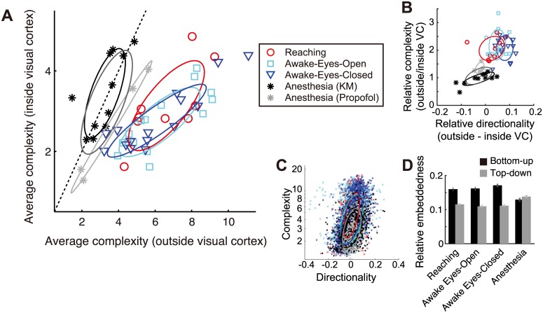
Brain-wide interactions generating complex neural dynamics are considered crucial for emergent cognitive functions. However, the irreducible nature of nonlinear and high-dimensional dynamical interactions challenges conventional reductionist approaches. We introduce a model-free method, based on embedding theorems in nonlinear state-space reconstruction, that permits a simultaneous characterization of complexity in local dynamics, directed interactions between brain areas, and how the complexity is produced by the interactions. We demonstrate this method in large-scale electrophysiological recordings from awake and anesthetized monkeys. The cross-embedding method captures structured interaction underlying cortex-wide dynamics that may be missed by conventional correlation-based analysis, demonstrating a critical role of time-series analysis in characterizing brain state. The method reveals a consciousness-related hierarchy of cortical areas, where dynamical complexity increases along with cross-area information flow. These findings demonstrate the advantages of the cross-embedding method in deciphering large-scale and heterogeneous neuronal systems, suggesting a crucial contribution by sensory-frontoparietal interactions to the emergence of complex brain dynamics during consciousness.
Overview
The claims and statistics of this paper haven’t been checked yet.
Free: it reads the open-access text and checks the first 5 claims that cite a source we can check. Create a free account to check every claim.
Integrity signals
Registry
Cites
Statistics
Figures




Verification
Claims the paper makes
The claims and statistics of this paper haven’t been checked yet.
Free: it reads the open-access text and checks the first 5 claims that cite a source we can check. Create a free account to check every claim.
Claims other papers make about this one
Each is checked against this paper’s own text: does it say what the citing paper says it does?
The check wasn’t confident either way, so it gives no verdict — never disputed.
In the citing paper
“IIT’s Φ cannot be easily computed from large-scale data, making it difficult to test the theory (for attempts, see Oizumi et al., 2016 and Tajima et al., 2015).”
From Conscious Processing and the Global Neuronal Workspace Hypothesis (2020) · cites this paper as Tajima et al., 2015
Experimental — accuracy not yet measured
Self-check
Percentages, sums and reported differences re-computed from the paper’s own numbers.
The self-check needs the paper’s full text.
Citations
Cites
Investigating causal relations by econometric models and cross-spectral methods
Granger, C. W. J. (1969) · Econometrica · doi:10.2307/1912791 · Cited by 22,989
A neural substrate of prediction and reward
Schultz, W., Dayan, P., & Montague, P. R. (1997) · Science · doi:10.1126/science.275.5306.1593 · Cited by 9,388 · cited 1×
“Embedding describes the observability of information in one brain area by another area, fulfilling a prerequisite for the actor-critic models of brain systems [58].”
BackgroundPermutation Entropy: A Natural Complexity Measure for Time Series
Bandt, C., & Pompe, B. (2002) · Physical Review Letters · doi:10.1103/physrevlett.88.174102 · Cited by 4,867 · cited 1×
“We compared the present complexitymeasure to the five other related measures (Materials and Methods): (i) correlation dimension [29], (ii) dimensionality derived from principle component analysis (PCA), (iii) permutation entropy [30,31], (iv) algorithmic (KolmogorovChaitin) complexity [32,33], and (v) the optimal embe…”
MethodCharacterization of Strange Attractors
Grassberger, P., & Procaccia, I. (1983) · Physical Review Letters · doi:10.1103/physrevlett.50.346 · Cited by 4,857 · cited 2×
“The correlation dimension was computed with the algorithm proposed by [29]; the PCA dimension was quantified by the number of dimension explaining 90% of the all variance; the permutation entropy was derived using the algorithm proposed by [31]; the algorithmic complexity was derived with the method proposed by [75];…”
MethodInvestigating Causal Relations by Econometric Models and Cross-Spectral Methods
Granger, C. W. J. (2010) · Essays in Econometrics · doi:10.1017/cbo9780511753978.002 · Cited by 4,762
Measuring Information Transfer
Schreiber, T. (2000) · Physical Review Letters · doi:10.1103/physrevlett.85.461 · Cited by 4,530 · cited 1×
“It is worth noting that detecting a clear causal relationship by Transfer entropy [69,70], Granger causality [71] or spectral Granger causality [72,73] is not straightforward unless the system’s dynamical properties are well known, due to the confounding effects of phase delay [74] or self-predictability in determinis…”
BackgroundDetermining embedding dimension for phase-space reconstruction using a geometrical construction
Kennel, M. B., Brown, R., & Abarbanel, H. D. I. (1992) · Physical Review A · doi:10.1103/physreva.45.3403 · Cited by 3,776 · cited 2×
“The complexity of dynamics concerning pairwise interaction was quantified using minimum embedding dimension d that yielded 95% of optimal estimation accuracy maxd ry;ŷðxt dÞ, which is an extension of the false-neighbor method [27,28,68] to the present cross-embedding.”
BackgroundMethodThalamocortical oscillations in the sleeping and aroused brain
Steriade, M., McCormick, D. A., & Sejnowski, T. J. (1993) · Science · doi:10.1126/science.8235588 · Cited by 3,564
Experimental and theoretical approaches to conscious processing
Dehaene, S., & Changeux, J.-P. (2011) · Neuron · doi:10.1016/j.neuron.2011.03.018 · Cited by 2,573
Detecting Causality in Complex Ecosystems
Sugihara, G., May, R., Ye, H., Hsieh, C.-H., Deyle, E., Fogarty, M., & Munch, S. (2012) · Science · doi:10.1126/science.1227079 · Cited by 2,539 · cited 10×
“However, the directionality of causality between as pair of nodes should be detected by a node asking the other node whether there is any asymmetry of observability (conditional entropy) of a node by the other node [21], even under some stochasticity due to system noise (S4 Fig).”
BackgroundMethodInfluentialMeasurement of Linear Dependence and Feedback between Multiple Time Series
Geweke, J. (1982) · Journal of the American Statistical Association · doi:10.1080/01621459.1982.10477803 · Cited by 2,060 · cited 1×
“It is worth noting that detecting a clear causal relationship by Transfer entropy [69,70], Granger causality [71] or spectral Granger causality [72,73] is not straightforward unless the system’s dynamical properties are well known, due to the confounding effects of phase delay [74] or self-predictability in determinis…”
BackgroundSauer, T., Yorke, J. A., & Casdagli, M. (1991) · Journal of Statistical Physics · doi:10.1007/bf01053745 · Cited by 2,045
An information integration theory of consciousness
Tononi, G. (2004) · BMC Neuroscience · doi:10.1186/1471-2202-5-42 · Cited by 1,958
Nonlinear forecasting as a way of distinguishing chaos from measurement error in time series
Sugihara, G., & May, R. M. (1990) · Nature · doi:10.1038/344734a0 · Cited by 1,932 · cited 4×
“) Note that in real data with a limited sample size, the accuracies sometimes did not have plateaus but have a peak followed by a gradual decrease [23].”
BackgroundMethodInfluentialSteriade, M., Nunez, A., & Amzica, F. (1993) · The Journal of Neuroscience · doi:10.1523/jneurosci.13-08-03252.1993 · Cited by 1,903
Context-dependent computation by recurrent dynamics in prefrontal cortex
Mante, V., Sussillo, D., Shenoy, K. V., & Newsome, W. T. (2013) · Nature · doi:10.1038/nature12742 · Cited by 1,847
Intrinsic functional architecture in the anaesthetized monkey brain
Vincent, J. L., Patel, G. H., Fox, M. D., Snyder, A. Z., Baker, J. T., Van Essen, D. C., Zempel, J. M., Snyder, L. H., Corbetta, M., & Raichle, M. E. (2007) · Nature · doi:10.1038/nature05758 · Cited by 1,786 · cited 2×
“This fact may explain why some studies [37,40–42] but not others [13,43] have reported changes in the resting-state functional connectivity depending on arousal level.”
MethodResultNeural population dynamics during reaching
Churchland, M. M., Cunningham, J. P., Kaufman, M. T., Foster, J. D., Nuyujukian, P., Ryu, S. I., & Shenoy, K. V. (2012) · Nature · doi:10.1038/nature11129 · Cited by 1,626
Tononi, G. (1998) · Science · doi:10.1126/science.282.5395.1846 · Cited by 1,561
Breakdown of cortical effective connectivity during sleep
Massimini, M., Ferrarelli, F., Huber, R., Esser, S. K., Singh, H., & Tononi, G. (2005) · Science · doi:10.1126/science.1117256 · Cited by 1,534
Consciousness as integrated information: a provisional manifesto
Tononi, G. (2008) · The Biological Bulletin · doi:10.2307/25470707 · Cited by 1,529 · cited 2×
“This can reconcile two contrasting views on conscious process—concerning whether conscious processes are localized to specific “workspace” areas [17,18] or distributed across the entire system [4,19,20]—from the viewpoint of information coding by dynamical systems.”
BackgroundResultWhole-brain functional imaging at cellular resolution using light-sheet microscopy
Ahrens, M. B., Orger, M. B., Robson, D. N., Li, J. M., & Keller, P. J. (2013) · Nature Methods · doi:10.1038/nmeth.2434 · Cited by 1,392
General anaesthesia: from molecular targets to neuronal pathways of sleep and arousal
Franks, N. P. (2008) · Nature Reviews Neuroscience · doi:10.1038/nrn2372 · Cited by 1,295
Alkire, M. T., Hudetz, A. G., & Tononi, G. (2008) · Science · doi:10.1126/science.1149213 · Cited by 1,245
Atmospheric Predictability as Revealed by Naturally Occurring Analogues
Lorenz, E. N. (1969) · Journal of the Atmospheric Sciences · doi:10.1175/1520-0469(1969)26<636:aparbn>2.0.co;2 · Cited by 1,076 · cited 3×
“Although the original protocol uses this delay-vector for subsequent nonlinear forecasting analysis [22,23,63], we found that it makes the results vulnerable to the time-scale heterogeneity in the system.”
BackgroundMethodThe MVGC multivariate Granger causality toolbox: A new approach to Granger-causal inference
Barnett, L., & Seth, A. K. (2014) · Journal of Neuroscience Methods · doi:10.1016/j.jneumeth.2013.10.018 · Cited by 1,044
A hierarchy of intrinsic timescales across primate cortex
Murray, J. D., Bernacchia, A., Freedman, D. J., Romo, R., Wallis, J. D., Cai, X., Padoa-Schioppa, C., Pasternak, T., Seo, H., Lee, D., et al. (2014) · Nature Neuroscience · doi:10.1038/nn.3862 · Cited by 990 · cited 2×
“If the estimate is systematically affected by those signal properties, it complicates the interpretation of the complexity measure because different brain areas are known to exhibit different timescales [24] and experimental observations inevitably involve noise.”
BackgroundThe neural correlate of (un)awareness: lessons from the vegetative state
Laureys, S. (2005) · Trends in Cognitive Sciences · doi:10.1016/j.tics.2005.10.010 · Cited by 813
(2014) · Progress in Molecular Biology and Translational Science · doi:10.1016/c2012-0-00157-3 · Cited by 799
Spatiotemporal Dynamics of Cortical Sensorimotor Integration in Behaving Mice
Ferezou, I., Haiss, F., Gentet, L. J., Aronoff, R., Weber, B., & Petersen, C. C. H. (2007) · Neuron · doi:10.1016/j.neuron.2007.10.007 · Cited by 697
Raichle, M. E. (2011) · Brain Connectivity · doi:10.1089/brain.2011.0019 · Cited by 672 · cited 1×
“The brain is a complex system with restless activity dynamics [1].”
BackgroundElectrophysiological correlates of the brain's intrinsic large-scale functional architecture
He, B. J., Snyder, A. Z., Zempel, J. M., Smyth, M. D., & Raichle, M. E. (2008) · Proceedings of the National Academy of Sciences · doi:10.1073/pnas.0807010105 · Cited by 670
Tagliazucchi, E., & Laufs, H. (2014) · Neuron · doi:10.1016/j.neuron.2014.03.020 · Cited by 644
Boveroux, P., Vanhaudenhuyse, A., Bruno, M.-A., Noirhomme, Q., Lauwick, S., Luxen, A., Degueldre, C., Plenevaux, A., Schnakers, C., Phillips, C., et al. (2010) · Anesthesiology · doi:10.1097/aln.0b013e3181f697f5 · Cited by 630
Sitt, J. D., King, J.-R., El Karoui, I., Rohaut, B., Faugeras, F., Gramfort, A., Cohen, L., Sigman, M., Dehaene, S., & Naccache, L. (2014) · Brain · doi:10.1093/brain/awu141 · Cited by 608
Logical basis for information theory and probability theory
Kolmogorov, A. (1968) · IEEE Transactions on Information Theory · doi:10.1109/tit.1968.1054210 · Cited by 592
A Pathway in Primate Brain for Internal Monitoring of Movements
Sommer, M. A., & Wurtz, R. H. (2002) · Science · doi:10.1126/science.1069590 · Cited by 565 · cited 1×
“While a similar concept has been proposed in terms of anatomical connectivity as an internal monitoring property [59], it has not been linked to neuronal dynamics.”
BackgroundFrom the connectome to brain function
Bargmann, C. I., & Marder, E. (2013) · Nature Methods · doi:10.1038/nmeth.2451 · Cited by 561 · cited 3×
“How brain-wide interaction produces specific dynamics underlying cognitive functions is a central question in neuroscience [2,3].”
BackgroundNeural Mechanisms of Object-Based Attention
Baldauf, D., & Desimone, R. (2014) · Science · doi:10.1126/science.1247003 · Cited by 536
Easily calculable measure for the complexity of spatiotemporal patterns
Kaspar, F., & Schuster, H. G. (1987) · Physical Review A · doi:10.1103/physreva.36.842 · Cited by 505 · cited 1×
“The correlation dimension was computed with the algorithm proposed by [29]; the PCA dimension was quantified by the number of dimension explaining 90% of the all variance; the permutation entropy was derived using the algorithm proposed by [31]; the algorithmic complexity was derived with the method proposed by [75];…”
MethodPreserved Feedforward But Impaired Top-Down Processes in the Vegetative State
Boly, M., Garrido, M. I., Gosseries, O., Bruno, M.-A., Boveroux, P., Schnakers, C., Massimini, M., Litvak, V., Laureys, S., & Friston, K. (2011) · Science · doi:10.1126/science.1202043 · Cited by 498
Transient Dynamics for Neural Processing
Rabinovich, M., Huerta, R., & Laurent, G. (2008) · Science · doi:10.1126/science.1155564 · Cited by 491 · cited 1×
“How the brain utilizes such temporally encoded information remains an open problem, nevertheless, temporal sequences in nonstationary attractor dynamics have been suggested to subserve behaviorally relevant information [60,61].”
BackgroundSejnowski, T. J., Koch, C., & Churchland, P. S. (1988) · Science · doi:10.1126/science.3045969 · Cited by 458
Cortical network functional connectivity in the descent to sleep
Larson-Prior, L. J., Zempel, J. M., Nolan, T. S., Prior, F. W., Snyder, A. Z., & Raichle, M. E. (2009) · Proceedings of the National Academy of Sciences · doi:10.1073/pnas.0900924106 · Cited by 450 · cited 1×
“This fact may explain why some studies [37,40–42] but not others [13,43] have reported changes in the resting-state functional connectivity depending on arousal level.”
ResultA robust method for detecting interdependences: application to intracranially recorded EEG
Arnhold, J., Grassberger, P., Lehnertz, K., & Elger, C. E. (1999) · Physica D: Nonlinear Phenomena · doi:10.1016/s0167-2789(99)00140-2 · Cited by 439
Propofol Anesthesia and Sleep: A High-Density EEG Study
Murphy, M., Bruno, M.-A., Riedner, B. A., Boveroux, P., Noirhomme, Q., Landsness, E. C., Brichant, J.-F., Phillips, C., Massimini, M., Laureys, S., et al. (2011) · Sleep · doi:10.1093/sleep/34.3.283 · Cited by 418
A Robust Method for Detecting Interdependences: Application to Intracranially Recorded EEGPreprint
Arnhold, J., Grassberger, P., Lehnertz, K., & Elger, C. E. (2013) · Cited by 412
Support for a synaptic chain model of neuronal sequence generation
Long, M. A., Jin, D. Z., & Fee, M. S. (2010) · Nature · doi:10.1038/nature09514 · Cited by 399 · cited 1×
“How the brain utilizes such temporally encoded information remains an open problem, nevertheless, temporal sequences in nonstationary attractor dynamics have been suggested to subserve behaviorally relevant information [60,61].”
BackgroundDirect test for determinism in a time series
Kaplan, D. T., & Glass, L. (1992) · Physical Review Letters · doi:10.1103/physrevlett.68.427 · Cited by 380 · cited 2×
“The complexity of dynamics concerning pairwise interaction was quantified using minimum embedding dimension d that yielded 95% of optimal estimation accuracy maxd ry;ŷðxt dÞ, which is an extension of the false-neighbor method [27,28,68] to the present cross-embedding.”
MethodInformation Sharing in the Brain Indexes Consciousness in Noncommunicative Patients
King, J.-R., Sitt, J. D., Faugeras, F., Rohaut, B., El Karoui, I., Cohen, L., Naccache, L., & Dehaene, S. (2013) · Current Biology · doi:10.1016/j.cub.2013.07.075 · Cited by 370 · cited 1×
“The unconscious (anesthetized) state was modeled by a network having only weak long-range coupling among the three clusters, but is moderately coupled within individual clusters (Fig 8A), which follows the experimental findings [40].”
Estimating Granger Causality from Fourier and Wavelet Transforms of Time Series Data
Dhamala, M., Rangarajan, G., & Ding, M. (2008) · Physical Review Letters · doi:10.1103/physrevlett.100.018701 · Cited by 346 · cited 1×
“It is worth noting that detecting a clear causal relationship by Transfer entropy [69,70], Granger causality [71] or spectral Granger causality [72,73] is not straightforward unless the system’s dynamical properties are well known, due to the confounding effects of phase delay [74] or self-predictability in determinis…”
BackgroundPractical considerations of permutation entropy: A tutorial review
Riedl, M., Müller, A., & Wessel, N. (2013) · The European Physical Journal Special Topics · doi:10.1140/epjst/e2013-01862-7 · Cited by 339 · cited 2×
“The correlation dimension was computed with the algorithm proposed by [29]; the PCA dimension was quantified by the number of dimension explaining 90% of the all variance; the permutation entropy was derived using the algorithm proposed by [31]; the algorithmic complexity was derived with the method proposed by [75];…”
MethodLehnertz, K., & Elger, C. E. (1995) · Electroencephalography and Clinical Neurophysiology · doi:10.1016/0013-4694(95)00071-6 · Cited by 325 · cited 2×
“the correlation dimension [11] or the algorithmic complexity [12]) and others evaluate neural interaction (e.”
BackgroundBeyond the Connectome: The Dynome
Kopell, N. J., Gritton, H. J., Whittington, M. A., & Kramer, M. A. (2014) · Neuron · doi:10.1016/j.neuron.2014.08.016 · Cited by 323
Connectivity Changes Underlying Spectral EEG Changes during Propofol-Induced Loss of Consciousness
Boly, M., Moran, R., Murphy, M., Boveroux, P., Bruno, M.-A., Noirhomme, Q., Ledoux, D., Bonhomme, V., Brichant, J.-F., Tononi, G., et al. (2012) · The Journal of Neuroscience · doi:10.1523/jneurosci.3769-11.2012 · Cited by 307
Ganguli, S., & Sompolinsky, H. (2012) · Annual Review of Neuroscience · doi:10.1146/annurev-neuro-062111-150410 · Cited by 256 · cited 1×
“It is also intuitively understandable that virtually any random projection does not break the topology of the attractor (except for special cases), which is a consequence of random projection theory [25].”
BackgroundFaes, L., Nollo, G., & Porta, A. (2011) · Physical Review E · doi:10.1103/physreve.83.051112 · Cited by 253 · cited 2×
“(B) The p-value distribution in transfer entropy, where we used nonuniform embedding-dimension technique [70] for a fair comparison.”
BackgroundMethodSpectral Signatures of Reorganised Brain Networks in Disorders of Consciousness
Chennu, S., Finoia, P., Kamau, E., Allanson, J., Williams, G. B., Monti, M. M., Noreika, V., Arnatkeviciute, A., Canales-Johnson, A., Olivares, F., et al. (2014) · PLoS Computational Biology · doi:10.1371/journal.pcbi.1003887 · Cited by 243
Thalamic deactivation at sleep onset precedes that of the cerebral cortex in humans
Magnin, M., Rey, M., Bastuji, H., Guillemant, P., Mauguière, F., & Garcia-Larrea, L. (2010) · Proceedings of the National Academy of Sciences · doi:10.1073/pnas.0909710107 · Cited by 230
Velly, L. J., Rey, M. F., Bruder, N. J., Gouvitsos, F. A., Witjas, T., Regis, J. M., Peragut, J. C., & Gouin, F. M. (2007) · Anesthesiology · doi:10.1097/01.anes.0000270734.99298.b4 · Cited by 217
Delay Embeddings for Forced Systems. I. Deterministic Forcing
Stark, J. (1999) · Journal of Nonlinear Science · doi:10.1007/s003329900072 · Cited by 212 · cited 1×
“It is a direct consequence of a mathematical theorem proven by Stark [26].”
BackgroundNonlinear prediction as a way of distinguishing chaos from random fractal sequences
Tsonis, A. A., & Elsner, J. B. (1992) · Nature · doi:10.1038/358217a0 · Cited by 203
Delay Embeddings for Forced Systems. II. Stochastic Forcing
Stark, J., Broomhead, D. S., Davies, M. E., & Huke, J. (2003) · Journal of Nonlinear Science · doi:10.1007/s00332-003-0534-4 · Cited by 179
False neighbors and false strands: A reliable minimum embedding dimension algorithm
Kennel, M. B., & Abarbanel, H. D. I. (2002) · Physical review. E, Statistical physics, plasmas, fluids, and related interdisciplinary topics · doi:10.1103/physreve.66.026209 · Cited by 173 · cited 4×
“The complexity of dynamics concerning pairwise interaction was quantified using minimum embedding dimension d that yielded 95% of optimal estimation accuracy maxd ry;ŷðxt dÞ, which is an extension of the false-neighbor method [27,28,68] to the present cross-embedding.”
BackgroundMethodInfluentialLee, U., Mashour, G. A., Kim, S., Noh, G.-J., & Choi, B.-M. (2009) · Consciousness and Cognition · doi:10.1016/j.concog.2008.10.005 · Cited by 141
Information-theoretic computation complexity
Chaitin, G. (1974) · IEEE Transactions on Information Theory · doi:10.1109/tit.1974.1055172 · Cited by 130
Causal density and integrated information as measures of conscious level
Seth, A. K., Barrett, A. B., & Barnett, L. (2011) · Philosophical Transactions of the Royal Society A: Mathematical, Physical and Engineering Sciences · doi:10.1098/rsta.2011.0079 · Cited by 129
INFORMATION-THEORETIC COMPUTATIONAL COMPLEXITY
Chaitin, G. J. (1987) · Information, Randomness & Incompleteness · doi:10.1142/9789814434058_0003 · Cited by 117 · cited 1×
“We compared the present complexitymeasure to the five other related measures (Materials and Methods): (i) correlation dimension [29], (ii) dimensionality derived from principle component analysis (PCA), (iii) permutation entropy [30,31], (iv) algorithmic (KolmogorovChaitin) complexity [32,33], and (v) the optimal embe…”
MethodNagasaka, Y., Shimoda, K., & Fujii, N. (2011) · PLoS ONE · doi:10.1371/journal.pone.0022561 · Cited by 104 · cited 1×
“The details on the recording apparatus have previously been reported [62], and part of the dataset is available online (http://neurotycho.”
BackgroundSelf-citationLarge-Scale Information Flow in Conscious and Unconscious States: an ECoG Study in Monkeys
Yanagawa, T., Chao, Z. C., Hasegawa, N., & Fujii, N. (2013) · PLoS ONE · doi:10.1371/journal.pone.0080845 · Cited by 82 · cited 2×
“We observed slow wave oscillations in the neural signal [42] as an additional confirmation of LOC.”
MethodSelf-citationIdentifying hidden common causes from bivariate time series: A method using recurrence plots
Hirata, Y., & Aihara, K. (2010) · Physical Review E · doi:10.1103/physreve.81.016203 · Cited by 71
Walling, P. T., & Hicks, K. N. (2006) · Anesthesiology · doi:10.1097/00000542-200611000-00013 · Cited by 48
Neural mechanisms of object-based attention
Baldauf, D., & Desimone, R. (2014) · Journal of Vision · doi:10.1167/14.10.1119 · Cited by 46
Reconstruction of Shared Nonlinear Dynamics in a Network
SAUER, T. D. (2004) · Physical Review Letters · doi:10.1103/physrevlett.93.198701 · Cited by 41
Method of false nearest neighbors: A cautionary note
Fredkin, D. R., & Rice, J. A. (1995) · Physical review. E, Statistical physics, plasmas, fluids, and related interdisciplinary topics · doi:10.1103/physreve.51.2950 · Cited by 40 · cited 2×
“This problem does not arise after the effect of signal autocorrelation [67,68] is eliminated by applying the above-mentioned coordinate-randomization procedure.”
BackgroundMethodvan den Broek, P. L. C., van Rijn, C. M., van Egmond, J., Coenen, A. M. L., & Booij, L. H. D. J. (2006) · European Journal of Anaesthesiology · doi:10.1017/s0265021505001857 · Cited by 26
Algorithmic complexity as an index of cortical function in awake and pentobarbital-anesthetized rats
Shaw, F.-Z., Chen, R., Tsao, H., & Yen, C. (1999) · Journal of Neuroscience Methods · doi:10.1016/s0165-0270(99)00133-8 · Cited by 25 · cited 1×
“the correlation dimension [11] or the algorithmic complexity [12]) and others evaluate neural interaction (e.”
BackgroundConfounding Effects of Phase Delays on Causality Estimation
Vakorin, V. A., Mišić, B., Krakovska, O., Bezgin, G., & McIntosh, A. R. (2013) · PLoS ONE · doi:10.1371/journal.pone.0053588 · Cited by 22 · cited 1×
“It is worth noting that detecting a clear causal relationship by Transfer entropy [69,70], Granger causality [71] or spectral Granger causality [72,73] is not straightforward unless the system’s dynamical properties are well known, due to the confounding effects of phase delay [74] or self-predictability in determinis…”
Background
Research works printed but not linked: 2
- M Riedl, 2013, Practical considerations of permutation entropy, Eur Phys J, 222, 249
- AN Kolmogorov, 1965, Three approaches to the definition of the concept of quantity of information, IEEE Trans Inf Theory, 14, 662
Cited by
Conscious Processing and the Global Neuronal Workspace Hypothesis
Mashour, G. A., Roelfsema, P., Changeux, J.-P., & Dehaene, S. (2020) · Neuron · doi:10.1016/j.neuron.2020.01.026 · Cited by 1,164
“IIT’s F cannot be easily computed from large-scale data, making it difficult to test the theory (for attempts, see Oizumi et al., 2016 and Tajima et al., 2015).”
MethodSocial Influence as Intrinsic Motivation for Multi-Agent Deep Reinforcement Learning
Jaques, N., Lazaridou, A., Hughes, E., Gülçehre, Ç., Ortega, P. A., Strouse, D., Leibo, J. Z., & de Freitas, N. (2018) · arXiv (Cornell University) · doi:10.48550/arxiv.1810.08647 · Cited by 241
“The limitation of this approach is that CCM estimates of causality are known to degrade in the presence of stochastic effects (Tajima et al., 2015).”
BackgroundGordon, N., Tsuchiya, N., Koenig‐Robert, R., & Hohwy, J. (2019) · PLoS Biology · doi:10.1371/journal.pbio.3000233 · Cited by 88
Consciousness & Brain Functional Complexity in Propofol Anaesthesia
Varley, T. F., Luppi, A. I., Pappas, I., Naçi, L., Ram, A., Owen, A. M., Menon, D. K., & Stamatakis, E. A. (2020) · Scientific Reports · doi:10.1038/s41598-020-57695-3 · Cited by 93
Recent developments in empirical dynamic modelling
Munch, S. B., Rogers, T. L., & Sugihara, G. (2022) · Methods in Ecology and Evolution · doi:10.1111/2041-210x.13983 · Cited by 98
“Alternatively, the time- scale problem can be circumvented using an ensemble of randomly generated delay vectors (see e.g. Tajima et al., 2015).”
Method
Metadata
- Authors
- Tajima, S., Yanagawa, T., Fujii, N., & Toyoizumi, T.
- Affiliations
- University of Geneva (CH)
- RIKEN Center for Brain Science (JP)
- Tokyo Institute of Technology (JP)
- Corresponding author
- Tajima, Satohiro
- Yanagawa, Toru
- Fujii, Naotaka
- Toyoizumi, Taro
- Venue
- PLOS Computational Biology
- Publisher
- Public Library of Science (PLoS)
- Published
- 2015-11-19
- Volume
- 11
- Issue
- 11
- Pages
- e1004537
- ISSN
- 1553-734X (ISSN-L)
- 1553-7358
- PMC
- PMC4652869
- OpenAlex
- W2173362524
- Cited by
- 76
- References
- 78
- Citations by year
- 2026: 2 · 2025: 5 · 2024: 8 · 2023: 9 · 2022: 8 · 2021: 5 · 2020: 12 · 2019: 7 · 2018: 6 · 2017: 11 · 2016: 2 · 2015: 1
- FWCI
- 4.01
- Type
- journal article
- Language
- en
- Open access
- gold
- doi.org
- Licence
- Locations
- PLoS Computational Biology (publishedVersion, cc-by)
- Europe PMC (PubMed Central) (publishedVersion, cc-by)
- PubMed Central (publishedVersion, cc-by)
- PubMed (publishedVersion)
- RePEc: Research Papers in Economics (submittedVersion)
- DOAJ (DOAJ: Directory of Open Access Journals) (submittedVersion, cc-by-sa)
- Figshare (submittedVersion, cc-by)
- Funders
- Japan Agency for Medical Research and Development
- Japan Society for the Promotion of Science
- RIKEN
- RIKEN Brain Science Institute
- Topics
- Life Sciences › Neuroscience › Cognitive Neuroscience › Neural dynamics and brain function
- Life Sciences › Neuroscience › Cognitive Neuroscience › Functional Brain Connectivity Studies
- Physical Sciences › Physics and Astronomy › Statistical and Nonlinear Physics › Chaos control and synchronization
- Keywords
- consciousness, dynamical complexity, cortical hierarchy, information flow, electrophysiological recording, model-independent analysis
- MeSH terms
- Algorithms, Animals, Brain, Consciousness, Electroencephalography, Macaca, Wakefulness, Computational Biology
About these checks
Registry, retraction, Cites and statistics results are computed, not judged, with one exception: a printed reference that no index lists is read once by a model before it counts as a citation error. Claims are extracted by a model and kept only when their quote appears verbatim in the text; each cited source is then checked, with a model’s help, for whether it says what the claim relies on. Those verdicts can be wrong — read the claim’s quote and the cited source before relying on one.
Statistics and arithmetic are recomputed, not judged.
Confidence bands are shown only for fields calibrated on our annotated test set. None is calibrated yet, so no band is shown.
What counts as a claim ›How we measure confidence ›How we check this ›
Are you an author, or do you see a problem with this page? Request a review
Data sources
Bibliographic data: Semantic Scholar, OpenAlex, Crossref.
Contains information from the Semantic Scholar Academic Graph Datasets, made available under the ODC Attribution License (ODC-BY 1.0).
Semantic Scholar’s data is described in: Kinney, R., et al. (2023). The Semantic Scholar Open Data Platform. arXiv:2301.10140.
