

The DOI matches its Crossref record; 6 of the 6 references it cites were found in a registry or an index.
Perturbing a quantum black hole
Abstract
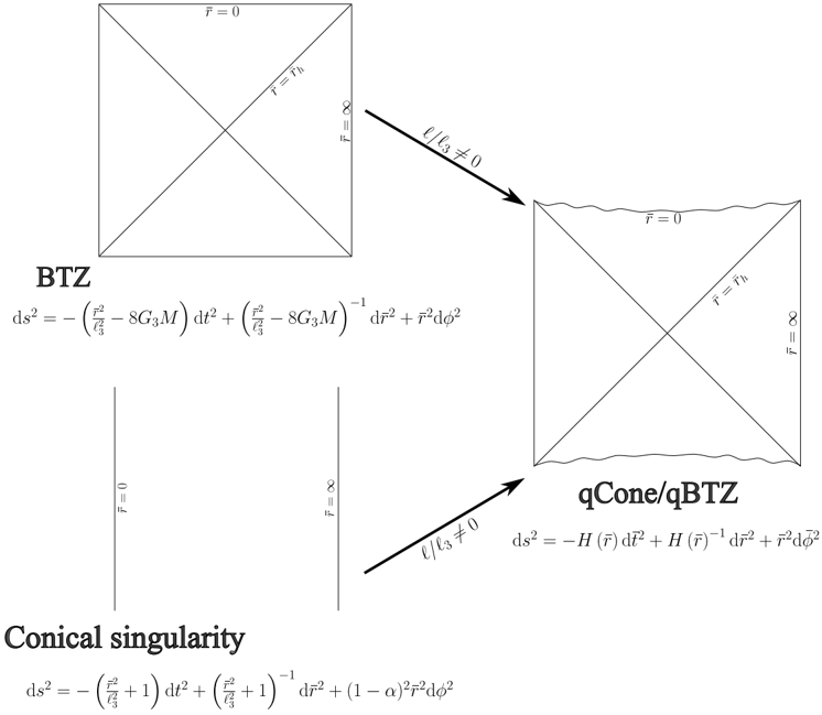
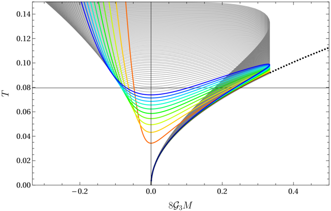
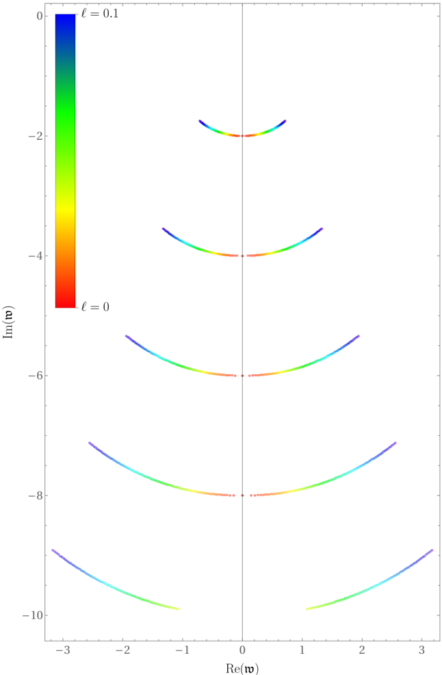
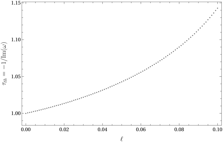
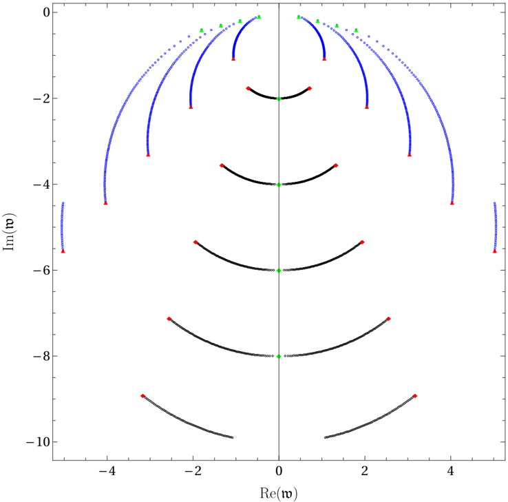
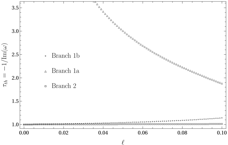
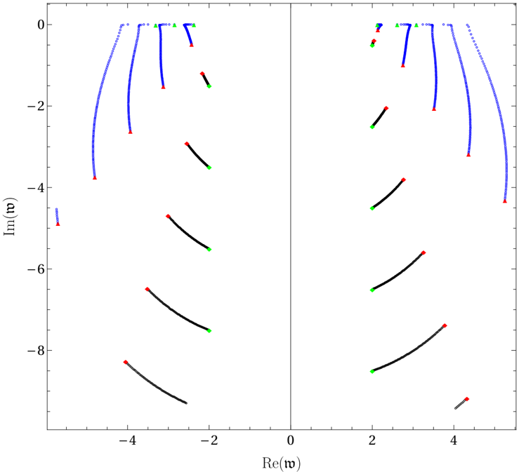
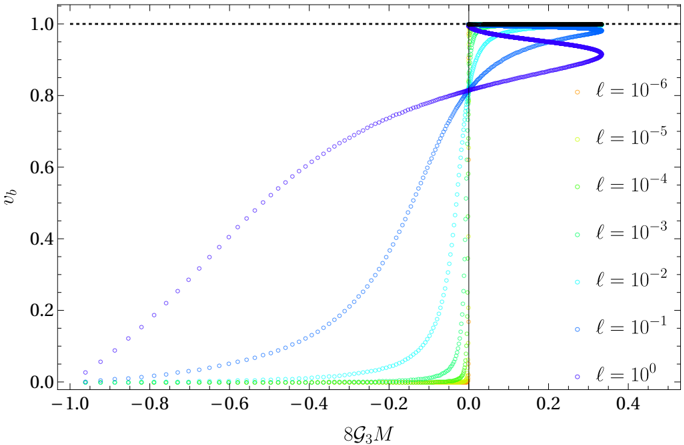
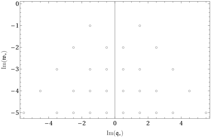
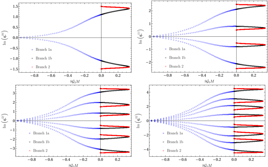
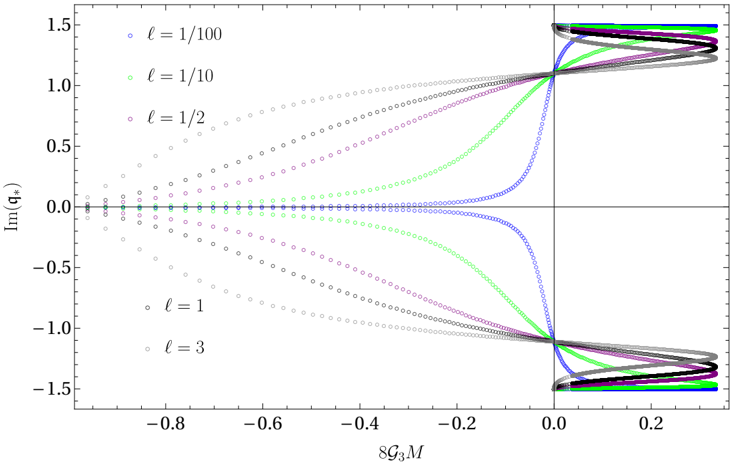
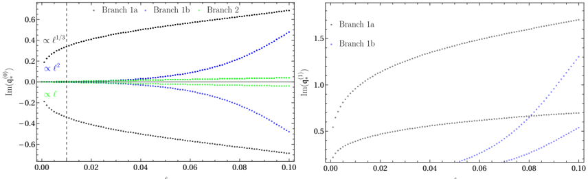
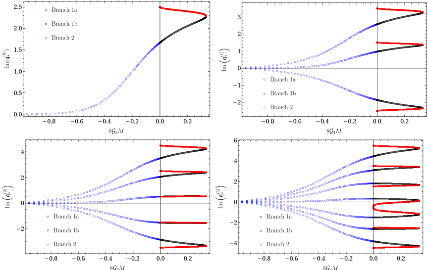
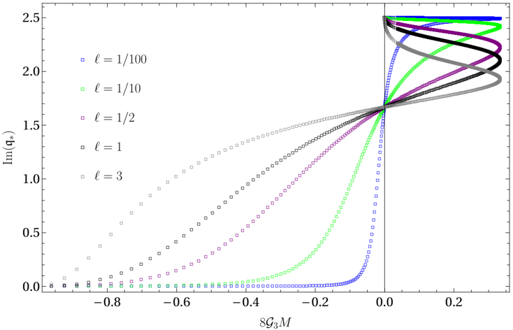
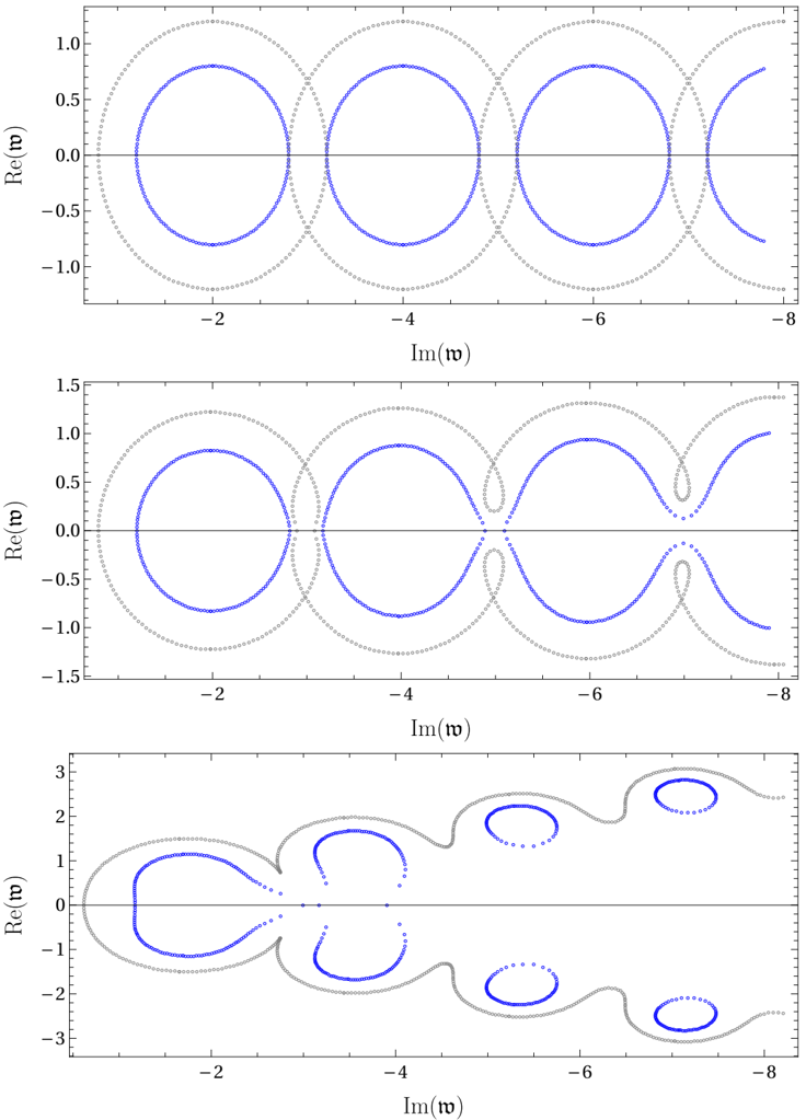
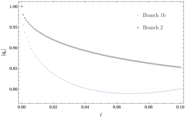
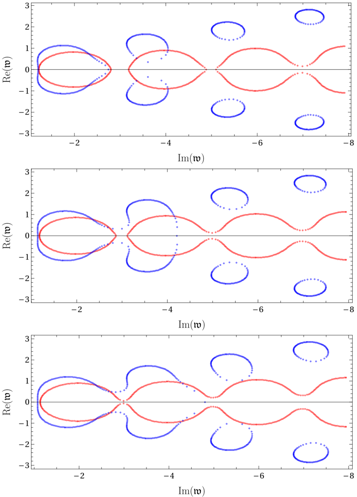
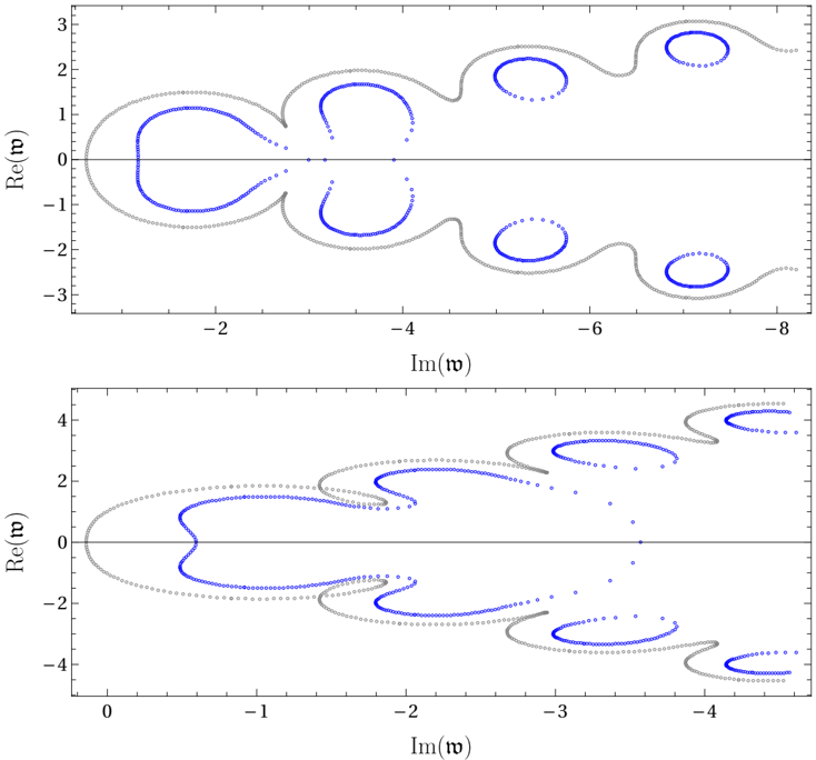
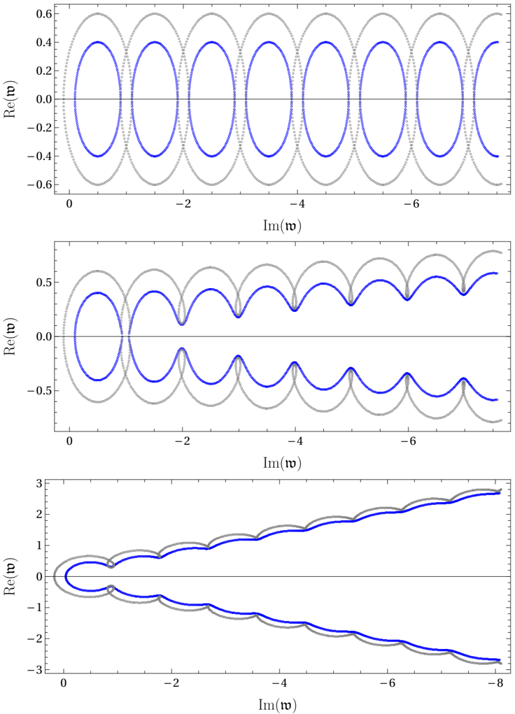
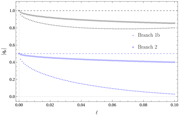
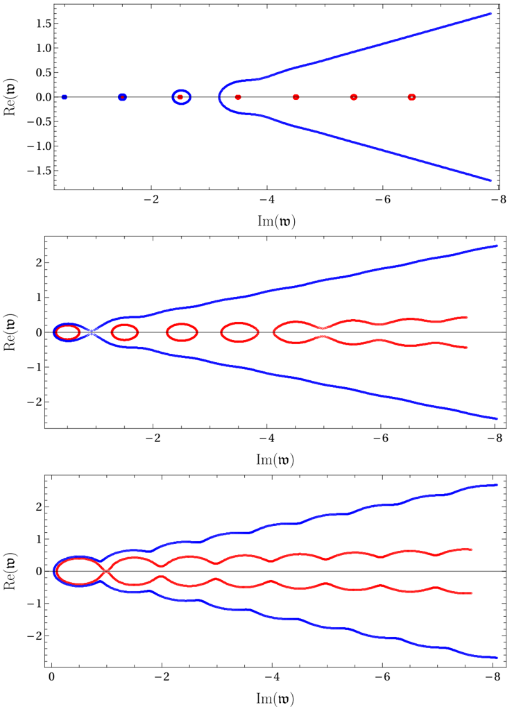
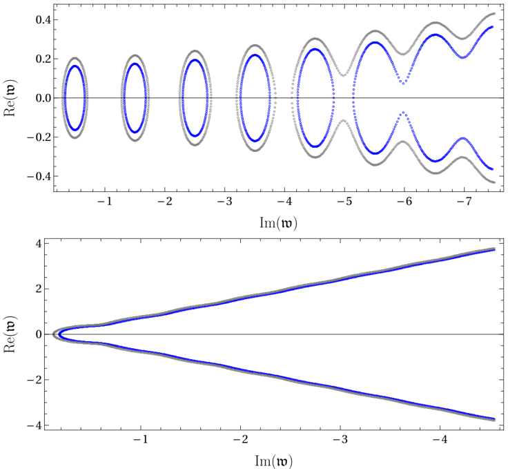
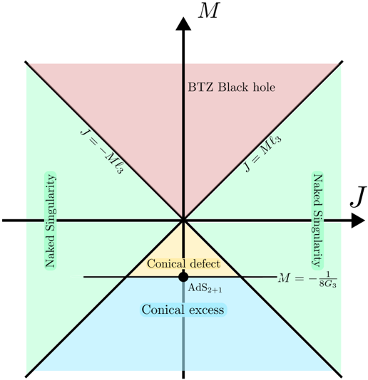
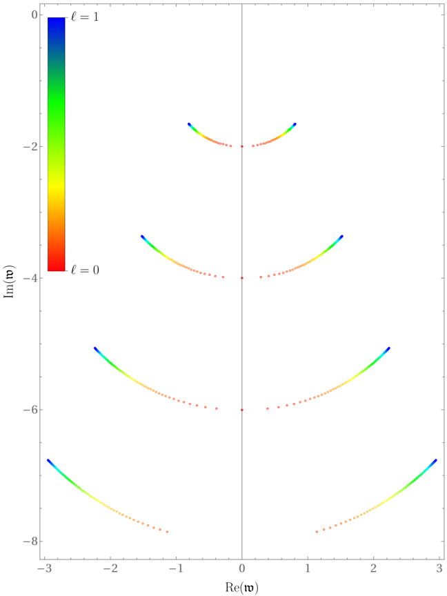
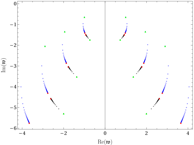
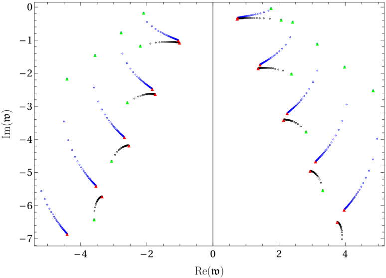
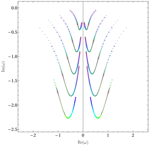
A bstract: We analyze the analytic structure of correlators in the field theory dual to the quantum Bañados-Teitelboim-Zanelli (qBTZ) black hole, a braneworld model incorporating exact backreaction from quantum conformal matter. We first compute the quasi-normal mode (QNM) spectrum of operators with dimension ∆ and spin s = 0, ±1/2. The leading QNMs and their overtones display qualitatively different behavior depending on the branch of qBTZ solution, which corresponds to distinct CFT states: branch 1 is a conical singularity dressed with a horizon while branch 2 is a quantum-corrected BTZ black hole. Consequently, the relaxation of probe matter effectively differentiates the CFT states and identifies the corresponding bulk descriptions. We then turn to pole-skipping locations where Green’s functions are not unique. At these points, frequency is proportional to temperature, but momentum exhibits complex temperature dependence due to quantum effects. Under the assumption that the pole-skipping point closest to the origin reflects quantum chaos, we infer the likely behavior of the quantum Lyapunov exponent and butterfly velocity in the dual theory. Finally, we examine pole collisions in complex momentum space, showing that quantum corrections imprint a unique signature on the analytic structure of the poles in retarded Green’s functions, resulting in level-crossing phenomena that differ notably from the level-touching phenomena in the uncorrected BTZ geometry.
Overview
The claims and statistics of this paper haven’t been checked yet.
Run the check — free, no account needed. It reads the open-access text and checks the sources it cites.
Integrity signals
Registry
Cites
Statistics
Figures
Verification
Claims the paper makes
The claims and statistics of this paper haven’t been checked yet.
Run the check — free, no account needed. It reads the open-access text and checks the sources it cites.
Claims other papers make about this one
Each is checked against this paper’s own text: does it say what the citing paper says it does?
The source backs part of the claim, not all of it — or backs it for a different population, condition or comparison.
In the citing paper
“Considering probe fields of brane localized matter, dual to CFT operators with conformal dimension ∆ ∈ [1,2] and spin s = 0, ±1/2, it was found that the QNMs and their overtones exhibit qualitatively different behavior depending on the branch of the qBTZ solution selected.”
From Three-Dimensional Quantum Black Holes: A Primer (2024) · cites this paper as [317]
Experimental — accuracy not yet measuredThe cited source says what the claim attributes to it.
In the citing paper
“A detailed study of QNMs of the quantum BTZ black hole provides some preliminary insights [317].”
From Three-Dimensional Quantum Black Holes: A Primer (2024) · cites this paper as [317]
In the citing paper
“Specifically, for the quantum BTZ black hole, the momentum of the pole-skipping points exhibits a non-trivial dependence on the parameter controlling the strength of backreaction.”
From Three-Dimensional Quantum Black Holes: A Primer (2024) · cites this paper as [317]
In the citing paper
“The pole structure of retarded two-point CFT correlators dual to quantum BTZ QNMs, moreover, exhibits a markedly different behavior than its classical counterpart [317].”
From Three-Dimensional Quantum Black Holes: A Primer (2024) · cites this paper as [317]
In the citing paper
“Further, by studying pole collisions in complex momentum space, quantum corrections have a significant impact on the analytic structure of the poles of retarded Green's functions.”
From Three-Dimensional Quantum Black Holes: A Primer (2024) · cites this paper as [317]
Self-check
Percentages, sums and reported differences re-computed from the paper’s own numbers.
The self-check needs the paper’s full text.
Citations
Cites
Quasinormal modes of AdS black holes and the approach to thermal equilibrium
Horowitz, G. T., & Hubeny, V. E. (2000) · Physical Review D · doi:10.1103/physrevd.62.024027 · Cited by 926
The Page curve of Hawking radiation from semiclassical geometry
Almheiri, A., Mahajan, R., Maldacena, J., & Zhao, Y. (2020) · Journal of High Energy Physics · doi:10.1007/jhep03(2020)149 · Cited by 898
Shenker, S. H., & Stanford, D. (2015) · Journal of High Energy Physics · doi:10.1007/jhep05(2015)132 · Cited by 604
Scalar, electromagnetic, and Weyl perturbations of BTZ black holes: Quasinormal modes
Cardoso, V., & Lemos, J. P. S. (2001) · Physical Review D · doi:10.1103/physrevd.63.124015 · Cited by 372
Birmingham, D. (2001) · Physical Review D · doi:10.1103/physrevd.64.064024 · Cited by 222
Three-Dimensional Quantum Black Holes: A Primer
Panella, E., Pedraza, J. F., & Svesko, A. (2024) · Universe · doi:10.3390/universe10090358 · Cited by 24
Self-citation
Research works printed but not linked: 118
- E. Witten, Anti-de Sitter space and holography, Adv. Theor. Math. Phys. 2 (1998) 253 [hep-th/9802150] [INSPIRE]. · DOI · Paper page
- S.S. Gubser, I.R. Klebanov and A.M. Polyakov, Gauge theory correlators from noncritical string theory, Phys. Lett. B 428 (1998) 105 [hep-th/9802109] [INSPIRE]. · DOI · Paper page
- T.R. Govindarajan and V. Suneeta, Quasinormal modes of AdS black holes: A Superpotential approach, Class. Quant. Grav. 18 (2001) 265 [gr-qc/0007084] [INSPIRE]. · DOI
- D. Birmingham, I. Sachs and S.N. Solodukhin, Conformal field theory interpretation of black hole quasinormal modes, Phys. Rev. Lett. 88 (2002) 151301 [hep-th/0112055] [INSPIRE]. · DOI · Paper page
- D.T. Son and A.O. Starinets, Minkowski space correlators in AdS / CFT correspondence: Recipe and applications, JHEP 09 (2002) 042 [hep-th/0205051] [INSPIRE]. · DOI · Paper page
- P. Kovtun, D.T. Son and A.O. Starinets, Viscosity in strongly interacting quantum field theories from black hole physics, Phys. Rev. Lett. 94 (2005) 111601 [hep-th/0405231] [INSPIRE]. · DOI
- G. Policastro, D.T. Son and A.O. Starinets, From AdS / CFT correspondence to hydrodynamics, JHEP 09 (2002) 043 [hep-th/0205052] [INSPIRE]. · DOI
- G. Policastro, D.T. Son and A.O. Starinets, From AdS / CFT correspondence to hydrodynamics. 2. Sound waves, JHEP 12 (2002) 054 [hep-th/0210220] [INSPIRE]. · DOI
- M. Natsuume and T. Okamura, Holographic chaos, pole-skipping, and regularity, PTEP 2020 (2020) 013B07 [arXiv:1905.12014] [INSPIRE]. · DOI
- M. Natsuume and T. Okamura, Nonuniqueness of Green’s functions at special points, JHEP 12 (2019) 139 [arXiv:1905.12015] [INSPIRE]. · DOI
- M. Blake, R.A. Davison and D. Vegh, Horizon constraints on holographic Green’s functions, JHEP 01 (2020) 077 [arXiv:1904.12883] [INSPIRE]. · DOI
- S.H. Shenker and D. Stanford, Black holes and the butterfly effect, JHEP 03 (2014) 067 [arXiv:1306.0622] [INSPIRE]. · DOI · Paper page
- S. Grozdanov, K. Schalm and V. Scopelliti, Black hole scrambling from hydrodynamics, Phys. Rev. Lett. 120 (2018) 231601 [arXiv:1710.00921] [INSPIRE]. · DOI · Paper page
- B. Withers, Short-lived modes from hydrodynamic dispersion relations, JHEP 06 (2018) 059 [arXiv:1803.08058] [INSPIRE]. · DOI
- S. Grozdanov, P.K. Kovtun, A.O. Starinets and P. Tadić, Convergence of the Gradient Expansion in Hydrodynamics, Phys. Rev. Lett. 122 (2019) 251601 [arXiv:1904.01018] [INSPIRE]. · DOI
- S. Grozdanov, P.K. Kovtun, A.O. Starinets and P. Tadić, The complex life of hydrodynamic modes, JHEP 11 (2019) 097 [arXiv:1904.12862] [INSPIRE]. · DOI · Paper page
- M.P. Heller et al., Convergence of hydrodynamic modes: insights from kinetic theory and holography, SciPost Phys. 10 (2021) 123 [arXiv:2012.15393] [INSPIRE]. · DOI
- S. Grozdanov, Bounds on transport from univalence and pole-skipping, Phys. Rev. Lett. 126 (2021) 051601 [arXiv:2008.00888] [INSPIRE]. · DOI
- J. Carballo and B. Withers, Transient dynamics of quasinormal mode sums, JHEP 10 (2024) 084 [arXiv:2406.06685] [INSPIRE]. · DOI
- C. Pantelidou and B. Withers, Thermal three-point functions from holographic Schwinger-Keldysh contours, JHEP 04 (2023) 050 [arXiv:2211.09140] [INSPIRE]. · DOI
- S. Grozdanov and T. Lemut, Reconstruction of spectra and an algorithm based on the theorems of Darboux and Puiseux, JHEP 02 (2023) 131 [arXiv:2209.02788] [INSPIRE]. · DOI
- S. Grozdanov, T. Lemut and J.F. Pedraza, Reconstruction of the quasinormal spectrum from pole skipping, Phys. Rev. D 108 (2023) L101901 [arXiv:2308.01371] [INSPIRE]. · DOI
- D. Areán, D.G. Fariña and K. Landsteiner, Pseudospectra of holographic quasinormal modes, JHEP 12 (2023) 187 [arXiv:2307.08751] [INSPIRE]. · DOI
- B. Cownden, C. Pantelidou and M. Zilhão, The pseudospectra of black holes in AdS, JHEP 05 (2024) 202 [arXiv:2312.08352] [INSPIRE]. · DOI
- R. Emparan, G.T. Horowitz and R.C. Myers, Exact description of black holes on branes, JHEP 01 (2000) 007 [hep-th/9911043] [INSPIRE]. · DOI · Paper page
- R. Emparan, G.T. Horowitz and R.C. Myers, Exact description of black holes on branes. 2. Comparison with BTZ black holes and black strings, JHEP 01 (2000) 021 [hep-th/9912135] [INSPIRE]. · DOI · Paper page
- R. Emparan, A. Fabbri and N. Kaloper, Quantum black holes as holograms in AdS brane worlds, JHEP 08 (2002) 043 [hep-th/0206155] [INSPIRE]. · DOI · Paper page
- L. Randall and R. Sundrum, An alternative to compactification, Phys. Rev. Lett. 83 (1999) 4690 [hep-th/9906064] [INSPIRE]. · DOI · Paper page
- L. Randall and R. Sundrum, A large mass hierarchy from a small extra dimension, Phys. Rev. Lett. 83 (1999) 3370 [hep-ph/9905221] [INSPIRE]. · DOI · Paper page
- A. Karch and L. Randall, Locally localized gravity, JHEP 05 (2001) 008 [hep-th/0011156] [INSPIRE]. · DOI · Paper page
- A. Karch and L. Randall, Open and closed string interpretation of SUSY CFT’s on branes with boundaries, JHEP 06 (2001) 063 [hep-th/0105132] [INSPIRE]. · DOI · Paper page
- R. Emparan, A.M. Frassino and B. Way, Quantum BTZ black hole, JHEP 11 (2020) 137 [arXiv:2007.15999] [INSPIRE]. · DOI · Paper page
- R. Emparan et al., Black holes in dS3, JHEP 11 (2022) 073 [arXiv:2207.03302] [INSPIRE]. · DOI · Paper page
- E. Panella and A. Svesko, Quantum Kerr-de Sitter black holes in three dimensions, JHEP 06 (2023) 127 [arXiv:2303.08845] [INSPIRE]. · DOI · Paper page
- Y. Feng et al., Quantum charged black holes, JHEP 08 (2024) 184 [arXiv:2404.07192] [INSPIRE]. · DOI · Paper page
- A. Climent, R. Emparan and R.A. Hennigar, Chemical potential and charge in quantum black holes, JHEP 08 (2024) 150 [arXiv:2404.15148] [INSPIRE]. · DOI · Paper page
- H. Geng and A. Karch, Massive islands, JHEP 09 (2020) 121 [arXiv:2006.02438] [INSPIRE]. · DOI · Paper page
- H. Geng et al., Information Transfer with a Gravitating Bath, SciPost Phys. 10 (2021) 103 [arXiv:2012.04671] [INSPIRE]. · DOI
- H.Z. Chen et al., Quantum Extremal Islands Made Easy, Part I: Entanglement on the Brane, JHEP 10 (2020) 166 [arXiv:2006.04851] [INSPIRE]. · DOI
- H.Z. Chen et al., Quantum Extremal Islands Made Easy, Part II: Black Holes on the Brane, JHEP 12 (2020) 025 [arXiv:2010.00018] [INSPIRE]. · DOI · Paper page
- R. Emparan, A.M. Frassino, M. Sasieta and M. Tomašević, Holographic complexity of quantum black holes, JHEP 02 (2022) 204 [arXiv:2112.04860] [INSPIRE]. · DOI · Paper page
- A.M. Frassino, J.F. Pedraza, A. Svesko and M.R. Visser, Higher-Dimensional Origin of Extended Black Hole Thermodynamics, Phys. Rev. Lett. 130 (2023) 161501 [arXiv:2212.14055] [INSPIRE]. · DOI · Paper page
- B. Chen, Y. Liu and B. Yu, Holographic complexity of rotating quantum black holes, JHEP 01 (2024) 055 [arXiv:2307.15968] [INSPIRE]. · DOI
- M. Kolanowski and M. Tomašević, Singularities in 2D and 3D quantum black holes, JHEP 12 (2023) 102 [arXiv:2310.06014] [INSPIRE]. · DOI · Paper page
- A.M. Frassino, J.F. Pedraza, A. Svesko and M.R. Visser, Reentrant phase transitions of quantum black holes, Phys. Rev. D 109 (2024) 124040 [arXiv:2310.12220] [INSPIRE]. · DOI · Paper page
- C.V. Johnson and R. Nazario, Specific heats for quantum BTZ black holes in extended thermodynamics, Phys. Rev. D 110 (2024) 106004 [arXiv:2310.12212] [INSPIRE]. · DOI
- S.A. Hosseini Mansoori, J.F. Pedraza and M. Rafiee, Criticality and thermodynamic geometry of quantum BTZ black holes, Phys. Rev. D 111 (2025) 024012 [arXiv:2403.13063] [INSPIRE]. · DOI
- S.-P. Wu and S.-W. Wei, Thermodynamical topology of quantum BTZ black hole, Phys. Rev. D 110 (2024) 024054 [arXiv:2403.14167] [INSPIRE]. · DOI
- A.M. Frassino, J.V. Rocha and A.P. Sanna, Weak cosmic censorship and the rotating quantum BTZ black hole, JHEP 07 (2024) 226 [arXiv:2405.04597] [INSPIRE]. · DOI · Paper page
- A.M. Frassino, R.A. Hennigar, J.F. Pedraza and A. Svesko, Quantum Inequalities for Quantum Black Holes, Phys. Rev. Lett. 133 (2024) 181501 [arXiv:2406.17860] [INSPIRE]. · DOI · Paper page
- Z.-M. Xu, P.-P. Zhang, B. Wu and X. Zhang, Thermodynamic bounce effect in quantum BTZ black hole, JHEP 12 (2024) 181 [arXiv:2407.08241] [INSPIRE]. · DOI
- H. Chung, L. Randall, M.J. Rodriguez and O. Varela, Quasinormal ringing on the brane, Class. Quant. Grav. 33 (2016) 245013 [arXiv:1508.02611] [INSPIRE]. · DOI
- S. Bhattacharjee, S. Sarkar and A. Bhattacharyya, Scalar perturbations of black holes in Jackiw-Teitelboim gravity, Phys. Rev. D 103 (2021) 024008 [arXiv:2011.08179] [INSPIRE]. · DOI
- M. Casals, A. Fabbri, C. Martínez and J. Zanelli, Quantum dress for a naked singularity, Phys. Lett. B 760 (2016) 244 [arXiv:1605.06078] [INSPIRE]. · DOI
- M. Casals, A. Fabbri, C. Martínez and J. Zanelli, Quantum Backreaction on Three-Dimensional Black Holes and Naked Singularities, Phys. Rev. Lett. 118 (2017) 131102 [arXiv:1608.05366] [INSPIRE]. · DOI
- J.M. Maldacena, Eternal black holes in anti-de Sitter, JHEP 04 (2003) 021 [hep-th/0106112] [INSPIRE]. · DOI · Paper page
- G. Festuccia and H. Liu, Excursions beyond the horizon: Black hole singularities in Yang-Mills theories. I, JHEP 04 (2006) 044 [hep-th/0506202] [INSPIRE]. · DOI
- G. Festuccia and H. Liu, The arrow of time, black holes, and quantum mixing of large N Yang-Mills theories, JHEP 12 (2007) 027 [hep-th/0611098] [INSPIRE]. · DOI
- L. Fidkowski, V. Hubeny, M. Kleban and S. Shenker, The black hole singularity in AdS/CFT, JHEP 02 (2004) 014 [hep-th/0306170] [INSPIRE]. · DOI
- V.E. Hubeny, H. Liu and M. Rangamani, Bulk-cone singularities & signatures of horizon formation in AdS/CFT, JHEP 01 (2007) 009 [hep-th/0610041] [INSPIRE]. · DOI
- G.T. Horowitz, H. Leung, L. Queimada and Y. Zhao, Boundary signature of singularity in the presence of a shock wave, SciPost Phys. 16 (2024) 060 [arXiv:2310.03076] [INSPIRE]. · DOI
- E. Cáceres, A.K. Patra and J.F. Pedraza, Shock waves, black hole interiors and holographic RG flows, JHEP 07 (2024) 052 [arXiv:2311.12940] [INSPIRE]. · DOI
- J. Maldacena, S.H. Shenker and D. Stanford, A bound on chaos, JHEP 08 (2016) 106 [arXiv:1503.01409] [INSPIRE]. · DOI
- N. Abbasi and M. Kaminski, Constraints on quasinormal modes and bounds for critical points from pole-skipping, JHEP 03 (2021) 265 [arXiv:2012.15820] [INSPIRE]. · DOI
- C. Cartwright, Example of the convergence of hydrodynamics in strong external fields, Phys. Rev. D 110 (2024) 026021 [arXiv:2403.12638] [INSPIRE]. · DOI
- J.C. Schindler and A. Aguirre, Algorithms for the explicit computation of Penrose diagrams, Class. Quant. Grav. 35 (2018) 105019 [arXiv:1802.02263] [INSPIRE]. · DOI
- M. Briceño, C. Martínez and J. Zanelli, Central singularity of the BTZ geometries, Phys. Rev. D 110 (2024) 024075 [arXiv:2404.06552] [INSPIRE]. · DOI
- A. Castro, S. Detournay, N. Iqbal and E. Perlmutter, Holographic entanglement entropy and gravitational anomalies, JHEP 07 (2014) 114 [arXiv:1405.2792] [INSPIRE]. · DOI
- Y. Liu and A. Raju, Quantum Chaos in Topologically Massive Gravity, JHEP 12 (2020) 027 [arXiv:2005.08508] [INSPIRE]. · DOI
- M. Natsuume and T. Okamura, Pole-skipping and zero temperature, Phys. Rev. D 103 (2021) 066017 [arXiv:2011.10093] [INSPIRE]. · DOI
- M.A.G. Amano, C. Cartwright, M. Kaminski and J. Wu, Relativistic hydrodynamics under rotation: Prospects and limitations from a holographic perspective, Prog. Part. Nucl. Phys. 139 (2024) 104135 [arXiv:2308.11686] [INSPIRE]. · DOI
- M. Natsuume and T. Okamura, Pole-skipping with finite-coupling corrections, Phys. Rev. D 100 (2019) 126012 [arXiv:1909.09168] [INSPIRE]. · DOI
- J. de Boer, E. Llabrés, J.F. Pedraza and D. Vegh, Chaotic strings in AdS/CFT, Phys. Rev. Lett. 120 (2018) 201604 [arXiv:1709.01052] [INSPIRE]. · DOI
- M. Mezei, On entanglement spreading from holography, JHEP 05 (2017) 064 [arXiv:1612.00082] [INSPIRE]. · DOI
- D. Giataganas, U. Gürsoy and J.F. Pedraza, Strongly-coupled anisotropic gauge theories and holography, Phys. Rev. Lett. 121 (2018) 121601 [arXiv:1708.05691] [INSPIRE]. · DOI
- W. Fischler, V. Jahnke and J.F. Pedraza, Chaos and entanglement spreading in a non-commutative gauge theory, JHEP 11 (2018) 072 [Erratum ibid. 02 (2021) 149] [arXiv:1808.10050] [INSPIRE]. · DOI
- U. Gürsoy, M. Järvinen, G. Nijs and J.F. Pedraza, On the interplay between magnetic field and anisotropy in holographic QCD, JHEP 03 (2021) 180 [arXiv:2011.09474] [INSPIRE]. · DOI
- S. Eccles et al., Speeding up the spread of quantum information in chaotic systems, JHEP 12 (2021) 019 [arXiv:2108.12688] [INSPIRE]. · DOI
- R.M. Wald, General Relativity, Chicago Univ. Pr., Chicago, U.S.A. (1984) [https://doi.org/10.7208/chicago/9780226870373.001.0001] [INSPIRE]. · DOI · Paper page
- M. Natsuume and T. Okamura, Pole skipping in a non-black-hole geometry, Phys. Rev. D 108 (2023) 046012 [arXiv:2306.03930] [INSPIRE]. · DOI
- H.-S. Jeong, C.-W. Ji and K.-Y. Kim, Pole-skipping in rotating BTZ black holes, JHEP 08 (2023) 139 [arXiv:2306.14805] [INSPIRE]. · DOI
- M. Blake and R.A. Davison, Chaos and pole-skipping in rotating black holes, JHEP 01 (2022) 013 [arXiv:2111.11093] [INSPIRE]. · DOI
- M.A.G. Amano et al., Chaos and pole-skipping in a simply spinning plasma, JHEP 02 (2023) 253 [arXiv:2211.00016] [INSPIRE]. · DOI
- N. Abbasi and S. Tahery, Complexified quasinormal modes and the pole-skipping in a holographic system at finite chemical potential, JHEP 10 (2020) 076 [arXiv:2007.10024] [INSPIRE]. · DOI
- H.-S. Jeong, K.-Y. Kim and Y.-W. Sun, The breakdown of magneto-hydrodynamics near AdS2 fixed point and energy diffusion bound, JHEP 02 (2022) 006 [arXiv:2105.03882] [INSPIRE]. · DOI
- A. Jansen and C. Pantelidou, Quasinormal modes in charged fluids at complex momentum, JHEP 10 (2020) 121 [arXiv:2007.14418] [INSPIRE]. · DOI
- C. Cartwright et al., Convergence of hydrodynamics in a rotating strongly coupled plasma, Phys. Rev. D 108 (2023) 046014 [arXiv:2112.10781] [INSPIRE]. · DOI
- N. Iqbal and H. Liu, Real-time response in AdS/CFT with application to spinors, Fortsch. Phys. 57 (2009) 367 [arXiv:0903.2596] [INSPIRE]. · DOI
- S.S. Gubser, Absorption of photons and fermions by black holes in four-dimensions, Phys. Rev. D 56 (1997) 7854 [hep-th/9706100] [INSPIRE]. · DOI
- U.H. Danielsson, E. Keski-Vakkuri and M. Kruczenski, Black hole formation in AdS and thermalization on the boundary, JHEP 02 (2000) 039 [hep-th/9912209] [INSPIRE]. · DOI
- S.B. Giddings and A. Nudelman, Gravitational collapse and its boundary description in AdS, JHEP 02 (2002) 003 [hep-th/0112099] [INSPIRE]. · DOI
- J. Abajo-Arrastia, J. Aparicio and E. Lopez, Holographic Evolution of Entanglement Entropy, JHEP 11 (2010) 149 [arXiv:1006.4090] [INSPIRE]. · DOI
- V. Balasubramanian et al., Thermalization of Strongly Coupled Field Theories, Phys. Rev. Lett. 106 (2011) 191601 [arXiv:1012.4753] [INSPIRE]. · DOI
- V. Balasubramanian et al., Holographic Thermalization, Phys. Rev. D 84 (2011) 026010 [arXiv:1103.2683] [INSPIRE]. · DOI
- J. Aparicio and E. Lopez, Evolution of Two-Point Functions from Holography, JHEP 12 (2011) 082 [arXiv:1109.3571] [INSPIRE]. · DOI
- Y. Sekino and L. Susskind, Fast Scramblers, JHEP 10 (2008) 065 [arXiv:0808.2096] [INSPIRE]. · DOI · Paper page
- N. Lashkari et al., Towards the Fast Scrambling Conjecture, JHEP 04 (2013) 022 [arXiv:1111.6580] [INSPIRE]. · DOI
- H. van Dam and M.J.G. Veltman, Massive and massless Yang-Mills and gravitational fields, Nucl. Phys. B 22 (1970) 397 [INSPIRE]. · DOI · Paper page
- I.I. Kogan, S. Mouslopoulos and A. Papazoglou, The m → 0 limit for massive graviton in dS4 and AdS4: How to circumvent the van Dam-Veltman-Zakharov discontinuity, Phys. Lett. B 503 (2001) 173 [hep-th/0011138] [INSPIRE]. · DOI
- E.A. Bergshoeff, O. Hohm and P.K. Townsend, Massive Gravity in Three Dimensions, Phys. Rev. Lett. 102 (2009) 201301 [arXiv:0901.1766] [INSPIRE]. · DOI
- M. Alishahiha, A. Davody, A. Naseh and S.F. Taghavi, On butterfly effect in Higher Derivative Gravities, JHEP 11 (2016) 032 [arXiv:1610.02890] [INSPIRE]. · DOI
- M.M. Qaemmaqami, Butterfly effect in 3D gravity, Phys. Rev. D 96 (2017) 106012 [arXiv:1707.00509] [INSPIRE]. · DOI
- W.-H. Huang, Butterfly Velocity in Quadratic Gravity, Class. Quant. Grav. 35 (2018) 195004 [arXiv:1804.05527] [INSPIRE]. · DOI
- J. Barrat, A. Gimenez-Grau and P. Liendo, A dispersion relation for defect CFT, JHEP 02 (2023) 255 [arXiv:2205.09765] [INSPIRE]. · DOI
- L. Bianchi and D. Bonomi, Conformal dispersion relations for defects and boundaries, SciPost Phys. 15 (2023) 055 [arXiv:2205.09775] [INSPIRE]. · DOI
- M. Bañados, C. Teitelboim and J. Zanelli, The black hole in three-dimensional space-time, Phys. Rev. Lett. 69 (1992) 1849 [hep-th/9204099] [INSPIRE]. · DOI · Paper page
- M. Bañados, M. Henneaux, C. Teitelboim and J. Zanelli, Geometry of the (2+1) black hole, Phys. Rev. D 48 (1993) 1506 [Erratum ibid. 88 (2013) 069902] [gr-qc/9302012] [INSPIRE]. · DOI · Paper page
- O. Miskovic and J. Zanelli, Couplings between Chern-Simons gravities and 2p-branes, Phys. Rev. D 80 (2009) 044003 [arXiv:0901.0737] [INSPIRE]. · DOI
- O. Miskovic and J. Zanelli, On the negative spectrum of the 2+1 black hole, Phys. Rev. D 79 (2009) 105011 [arXiv:0904.0475] [INSPIRE]. · DOI
- W. Israel, Singular hypersurfaces and thin shells in general relativity, Nuovo Cim. B 44S10 (1966) 1 [Erratum ibid. 48 (1967) 463] [INSPIRE]. · DOI · Paper page
- K. Lanczos, Flächenhafte Verteilung der Materie in der Einsteinschen Gravitationstheorie, Annalen Phys. 379 (1924) 518 [INSPIRE]. · DOI
- E. Poisson, A Relativist’s Toolkit: The Mathematics of Black-Hole Mechanics, Cambridge University Press (2009) [https://doi.org/10.1017/CBO9780511606601] [INSPIRE]. · DOI · Paper page
- S. Cremonini, J.T. Liu and P. Szepietowski, Higher Derivative Corrections to R-charged Black Holes: Boundary Counterterms and the Mass-Charge Relation, JHEP 03 (2010) 042 [arXiv:0910.5159] [INSPIRE]. · DOI · Paper page
- A. Jansen, Overdamped modes in Schwarzschild-de Sitter and a Mathematica package for the numerical computation of quasinormal modes, Eur. Phys. J. Plus 132 (2017) 546 [arXiv:1709.09178] [INSPIRE]. · DOI
- M. Henneaux, Boundary terms in the AdS / CFT correspondence for spinor fields, in the proceedings of the International Meeting on Mathematical Methods in Modern Theoretical Physics (ISPM 98), Tbilisi, Georgia, September 05–18 (1998) [hep-th/9902137] [INSPIRE]. · arXiv
- N. Ceplak, K. Ramdial and D. Vegh, Fermionic pole-skipping in holography, JHEP 07 (2020) 203 [arXiv:1910.02975] [INSPIRE]. · DOI
- R.J. Walker, Algebraic curves, vol. 58, Springer (1950).
- C.T.C. Wall, Singular Points of Plane Curves, Cambridge University Press (2004) [https://doi.org/10.1017/cbo9780511617560]. · DOI
Cited by
Sorted by citations
Three-Dimensional Quantum Black Holes: A Primer
Panella, E., Pedraza, J. F., & Svesko, A. (2024) · Universe · doi:10.3390/universe10090358 · Cited by 24
Self-citation
Metadata
- Authors
- Cartwright, C., Gürsoy, U., Pedraza, J. F., & Planas, G. P.
- Affiliations
- Utrecht University
- Instituto de Física Teórica UAM/CSIC
- Venue
- Journal of High Energy Physics
- Published
- 2025-03-06
- Volume
- 2025
- Issue
- 3
- ISSN
- 1029-8479
- Cited by
- 7
- References
- 6
- Language
- en
About these checks
Registry, retraction, Cites and statistics results are computed, not judged, with one exception: a printed reference that no index lists is read once by a model before it counts as a citation error. Claims are extracted by a model and kept only when their quote appears verbatim in the text; each cited source is then checked, with a model’s help, for whether it says what the claim relies on. Those verdicts can be wrong — read the claim’s quote and the cited source before relying on one.
Statistics and arithmetic are recomputed, not judged.
Confidence bands are shown only for fields calibrated on our annotated test set. None is calibrated yet, so no band is shown.
What counts as a claim ›How we measure confidence ›How we check this ›
Are you an author, or do you see a problem with this page? Request a review
