

The Python’s Lunch: geometric obstructions to decoding Hawking radiation
Open accessThe DOI matches its Crossref record; 81 of the 81 references it cites were found in a registry or an index.
Abstract
A bstract: According to Harlow and Hayden [ arXiv:1301.4504 ] the task of distilling information out of Hawking radiation appears to be computationally hard despite the fact that the quantum state of the black hole and its radiation is relatively un-complex. We trace this computational difficulty to a geometric obstruction in the Einstein-Rosen bridge connecting the black hole and its radiation. Inspired by tensor network models, we conjecture a precise formula relating the computational hardness of distilling information to geometric properties of the wormhole — specifically to the exponential of the difference in generalized entropies between the two non-minimal quantum extremal surfaces that constitute the obstruction. Due to its shape, we call this obstruction the ‘Python’s Lunch’, in analogy to the reptile’s postprandial bulge.
Overview
The claims and statistics of this paper haven’t been checked yet.
Free: it reads the open-access text and checks the first 5 claims that cite a source we can check. Create a free account to check every claim.
Integrity signals
Registry
Cites
Statistics
Figures






Verification
Claims the paper makes
The claims and statistics of this paper haven’t been checked yet.
Free: it reads the open-access text and checks the first 5 claims that cite a source we can check. Create a free account to check every claim.
Claims other papers make about this one
Each is checked against this paper’s own text: does it say what the citing paper says it does?
The source backs part of the claim, not all of it — or backs it for a different population, condition or comparison.
In the citing paper
“In fact, for evaporating black holes, there is good reason to think that it is exponentially complicated [65,66].”
From Replica wormholes and the black hole interior (2022) · cites this paper as [66]
Experimental — accuracy not yet measuredThe cited source says what the claim attributes to it.
In the citing paper
“A remarkable geometric way of capturing this complexity was proposed in [236] based on the generic existence of non-minimal extremal surfaces forming a Python-lunch geometry (sandwiched between minimal extremal surfaces or behind one of them) and interpreting this geometry in terms of tensor network constructions.”
From Holographic spacetime, black holes and quantum error correcting codes: a review (2022) · cites this paper as [236]
The cited source says what the claim attributes to it.
In the citing paper
“In all cases, the inher-ent chaos in microstate dynamics should connect the Python's lunch geometric mechanism of generating exponential complexity [236] in encoding with the pseudorandomness mechanism discussed in [258].”
From Holographic spacetime, black holes and quantum error correcting codes: a review (2022) · cites this paper as [236]
Self-check
Percentages, sums and reported differences re-computed from the paper’s own numbers.
The self-check needs the paper’s full text.
Citations
Cites
A fast quantum mechanical algorithm for database search
Grover, L. K. (1996) · Proceedings of the twenty-eighth annual ACM symposium on Theory of computing - STOC '96 · doi:10.1145/237814.237866 · Cited by 8,830 · cited 1×
“In the previous subsection we argued that we can decode Hawking radiation by projecting out m qubits, and provided a version of a Grover search [14, 15] that allows to do this”
Method(1988) · Elsevier eBooks · doi:10.1016/c2013-0-11200-7 · Cited by 5,131
Quantum Mechanics Helps in Searching for a Needle in a Haystack
Grover, L. K. (1997) · Physical Review Letters · doi:10.1103/physrevlett.79.325 · Cited by 4,306 · cited 1×
“where C TN NlogN. 4.3 Post-selection is Superpolynomial In the previous subsection we argued that we can decode Hawking radiation by projecting out mqubits, and provided a version of a Grover search [14, 15] that allows to do this projection with a unitary that has complexity p 2m. Can we rule out the possibility that…”
BackgroundInfluentialRyu, S., & Takayanagi, T. (2006) · Physical Review Letters · doi:10.1103/physrevlett.96.181602 · Cited by 4,302 · cited 1×
“However, the covariant surface that is analogous to the minimal cut through a tensor network is the HRT surface [23, 24, 25], the minimal area extremal surface homologous to one end of the wormhole.”
BackgroundA covariant holographic entanglement entropy proposal
Hubeny, V. E., Rangamani, M., & Takayanagi, T. (2007) · Journal of High Energy Physics · doi:10.1088/1126-6708/2007/07/062 · Cited by 1,822 · cited 1×
“However, the covariant surface that is analogous to the minimal cut through a tensor network is the HRT surface [23, 24, 25], the minimal area extremal surface homologous to one end of the wormhole.”
BackgroundA Covariant Holographic Entanglement Entropy Proposal
Hubeny, V. E., Rangamani, M., & Takayanagi, T. (2007) · arXiv · doi:10.48550/arxiv.0705.0016 · Cited by 1,822 · cited 1×
“However, the covariant surface that is analogous to the minimal cut through a tensor network is the HRT surface [23, 24, 25], the minimal area extremal surface homologous to one end of the wormhole.”
BackgroundAverage entropy of a subsystem
Page, D. N. (1993) · Physical Review Letters · doi:10.1103/physrevlett.71.1291 · Cited by 1,578 · cited 1×
“n we will see how a Python’s Lunch explains the exponential diculty of decoding Hawking radiation. After the Page time an evaporating black hole is maximally entangled with its own Hawking radiation [30]. Harlow and Hayden [1] asked how hard it is to isolate a degree of freedom r in the radiation that is entangled wit…”
BackgroundAverage Entropy of a Subsystem
Page, D. N. (1993) · arXiv · doi:10.48550/arxiv.gr-qc/9305007 · Cited by 1,578 · cited 1×
“n we will see how a Python’s Lunch explains the exponential diculty of decoding Hawking radiation. After the Page time an evaporating black hole is maximally entangled with its own Hawking radiation [30]. Harlow and Hayden [1] asked how hard it is to isolate a degree of freedom r in the radiation that is entangled wit…”
BackgroundBlack Holes: Complementarity or Firewalls?
Almheiri, A., Marolf, D., Polchinski, J., & Sully, J. (2012) · arXiv · doi:10.48550/arxiv.1207.3123 · Cited by 1,471
Strengths and Weaknesses of Quantum Computing
Bennett, C. H., Bernstein, E., Brassard, G., & Vazirani, U. (1997) · SIAM Journal on Computing · doi:10.1137/s0097539796300933 · Cited by 1,470
Black holes: complementarity or firewalls?
Almheiri, A., Marolf, D., Polchinski, J., & Sully, J. (2013) · Journal of High Energy Physics · doi:10.1007/jhep02(2013)062 · Cited by 1,470
Black holes as mirrors: quantum information in random subsystems
Hayden, P., & Preskill, J. (2007) · Journal of High Energy Physics · doi:10.1088/1126-6708/2007/09/120 · Cited by 1,332 · cited 1×
“13 This is the Hayden-Preskill decoding task [32] and is also expected to be exponentially hard.”
BackgroundCool horizons for entangled black holes
Maldacena, J., & Susskind, L. (2013) · arXiv · doi:10.48550/arxiv.1306.0533 · Cited by 1,310 · cited 5×
“This new black hole is entangled with the first black hole, and the entanglement can be interpreted, according to ER=EPR [5], as a wormhole connecting them.”
BackgroundInfluentialSelf-citationCool horizons for entangled black holes
Maldacena, J., & Susskind, L. (2013) · Fortschritte der Physik · doi:10.1002/prop.201300020 · Cited by 1,304 · cited 5×
“This new black hole is entangled with the first black hole, and the entanglement can be interpreted, according to ER=EPR [5], as a wormhole connecting them.”
BackgroundInfluentialSelf-citationGeneralized gravitational entropy
Lewkowycz, A., & Maldacena, J. (2013) · Journal of High Energy Physics · doi:10.1007/jhep08(2013)090 · Cited by 1,183
A Covariant Holographic Entanglement Entropy ProposalPreprint
Hubeny, V. E., Rangamani, M., & Takayanagi, T. (2008) · Cited by 1,170
The stretched horizon and black hole complementarity
Susskind, L., Thorlacius, L., & Uglum, J. (1993) · Physical Review D · doi:10.1103/physrevd.48.3743 · Cited by 1,081
Self-citationBlack holes: Complementarity or firewalls?
Almheiri, A., Marolf, D., Polchinski, J., & Sully, J. (2013) · eScholarship (California Digital Library) · Cited by 978
Quantum corrections to holographic entanglement entropy
Faulkner, T., Lewkowycz, A., & Maldacena, J. (2013) · Journal of High Energy Physics · doi:10.1007/jhep11(2013)074 · Cited by 945 · cited 1×
“reference system instead of a late-time Hawking quantum. 12The idea of entanglement wedge reconstruction was originally conjectured in [40, 41, 28], and established in [42, 43, 44] using the ideas of [45, 46]. 13In this context, the entanglement wedge of the Hawking radiation is dened as the bulk domain of dependence…”
MethodReplica wormholes and the entropy of Hawking radiation
Almheiri, A., Hartman, T., Maldacena, J., Shaghoulian, E., & Tajdini, A. (2020) · Journal of High Energy Physics · doi:10.1007/jhep05(2020)013 · Cited by 910 · cited 1×
“lty in doing either task comes from the exponentially large restricted complexity of the combined state of the black hole and Hawking radiation. Building on earlier ideas in [33, 34], it was shown in [35, 36, 37, 38, 39] that the information-theoretic achievability (or otherwise) of the Hayden-Preskill and Harlow-Hayd…”
MethodThe Page curve of Hawking radiation from semiclassical geometry
Almheiri, A., Mahajan, R., Maldacena, J., & Zhao, Y. (2020) · Journal of High Energy Physics · doi:10.1007/jhep03(2020)149 · Cited by 898 · cited 2×
“conditions, as in [36, 37].”
MethodHolographic Complexity Equals Bulk Action?
Brown, A. R., Roberts, D. A., Susskind, L., Swingle, B., & Zhao, Y. (2016) · Physical Review Letters · doi:10.1103/physrevlett.116.191301 · Cited by 852 · cited 1×
“volume of the maximal-volume slice [2], and the action of the Wheeler-de Witt patch [3, 4].”
BackgroundSelf-citationQuantum extremal surfaces: holographic entanglement entropy beyond the classical regime
Engelhardt, N., & Wall, A. C. (2015) · Journal of High Energy Physics · doi:10.1007/jhep01(2015)073 · Cited by 836
(1996) · Cited by 824
Entanglement as Topology: Hopf Linking as the Geometric Origin of Quantum Correlation
Novickis, A. (2026) · doi:10.5281/zenodo.20549411 · Cited by 821
The entropy of bulk quantum fields and the entanglement wedge of an evaporating black hole
Almheiri, A., Engelhardt, N., Marolf, D., & Maxfield, H. (2019) · Journal of High Energy Physics · doi:10.1007/jhep12(2019)063 · Cited by 818 · cited 10×
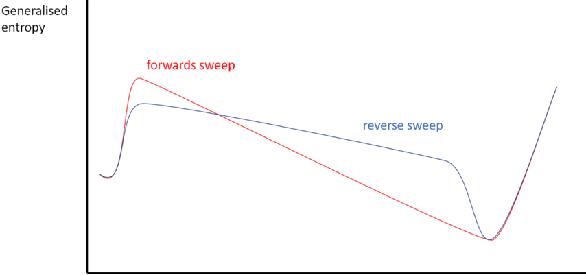
“However, the bulge surface that corresponds to the maximum size in the ‘forwards sweep’ was briefly discussed in [36].”
BackgroundMethodResultInfluentialReplica wormholes and the black hole interior
Penington, G., Shenker, S. H., Stanford, D., & Yang, Z. (2019) · arXiv · doi:10.48550/arxiv.1911.11977 · Cited by 809
Self-citationReplica wormholes and the black hole interior
Penington, G., Shenker, S. H., Stanford, D., & Yang, Z. (2022) · Journal of High Energy Physics · doi:10.1007/jhep03(2022)205 · Cited by 807
Self-citationBulk locality and quantum error correction in AdS/CFT
Almheiri, A., Dong, X., & Harlow, D. (2015) · Journal of High Energy Physics · doi:10.1007/jhep04(2015)163 · Cited by 802
Computational complexity and black hole horizons
Susskind, L. (2016) · Fortschritte der Physik · doi:10.1002/prop.201500092 · Cited by 767 · cited 2×
“volume of the maximal-volume slice [2], and the action of the Wheeler-de Witt patch [3, 4].”
BackgroundSelf-citationThe Page curve of Hawking radiation from semiclassical geometry
Almheiri, A., Mahajan, R., Maldacena, J., & Zhao, Y. (2019) · arXiv · doi:10.48550/arxiv.1908.10996 · Cited by 748 · cited 2×
“conditions, as in [36, 37].”
MethodSimulating Hamiltonian Dynamics with a Truncated Taylor Series
Berry, D. W., Childs, A. M., Cleve, R., Kothari, R., & Somma, R. D. (2015) · Physical Review Letters · doi:10.1103/physrevlett.114.090502 · Cited by 742 · cited 2×
“There are also other known lower bounds for more general classes of algorithms that perform amplitude amplification [20, 21, 22] and which are closely related to our state-independent protocol from Appendix A.”
BackgroundOperator Spreading in Random Unitary Circuits
Nahum, A., Vijay, S., & Haah, J. (2018) · Physical Review X · doi:10.1103/physrevx.8.021014 · Cited by 738 · cited 1×
“Modeling black holes as a quantum computer has been extremely fruitful in the study of quantum information scrambling [6, 7], onset of random matrix behavior [8] and derivation of the RT formula [9].”
BackgroundThe entropy of bulk quantum fields and the entanglement wedge of an evaporating black hole
Almheiri, A., Engelhardt, N., Marolf, D. M., & Maxfield, H. (2019) · eScholarship (California Digital Library) · Cited by 734
Complexity, action, and black holes
Brown, A. R., Roberts, D. A., Susskind, L., Swingle, B., & Zhao, Y. (2016) · Physical Review D · doi:10.1103/physrevd.93.086006 · Cited by 640 · cited 5×
“r end surface. It is given by C R= O texp h1 2 S rad + A 0 A hor 4G N i : (5.5) The factor of there comes from the volume of the lunch, which controls C TN according to the conjectures of Refs. [2, 3, 4]. The rst phase transition happens at the Page time, where the EW surface becomes nonempty. This means that the larg…”
BackgroundMethodInfluentialSelf-citationGrover’s quantum searching algorithm is optimal
Zalka, C. (1999) · Physical Review A · doi:10.1103/physreva.60.2746 · Cited by 635 · cited 1×
“h a speed up would be to change the coecient in the exponent of the conjecture Eq. 4.6 from 1/2 to 1/3.) It has been proved that Grover search amongst ditems cannot be implemented faster than ˇ 4 p d[17, 18, 19],9 but we have an advantage not available in the Grover task, which is that we know in advance which nal sta…”
BackgroundInfluentialHolographic duality from random tensor networks
Hayden, P., Nezami, S., Qi, X.-L., Thomas, N., Walter, M., & Yang, Z. (2016) · Journal of High Energy Physics · doi:10.1007/jhep11(2016)009 · Cited by 599 · cited 1×
“Modeling black holes as a quantum computer has been extremely fruitful in the study of quantum information scrambling [6, 7], onset of random matrix behavior [8] and derivation of the RT formula [9].”
BackgroundMaximin surfaces, and the strong subadditivity of the covariant holographic entanglement entropy
Wall, A. C. (2014) · Classical and Quantum Gravity · doi:10.1088/0264-9381/31/22/225007 · Cited by 545 · cited 5×
“We use ‘maximin’ techniques [28, 29] to sketch an argument that almost all spacetimes with more than one extremal surface will contain a Python’s Lunch.”
BackgroundMethodResultInfluentialGilyén, A., Su, Y., Low, G. H., & Wiebe, N. (2019) · Proceedings of the 51st Annual ACM SIGACT Symposium on Theory of Computing · doi:10.1145/3313276.3316366 · Cited by 542 · cited 2×
“(9)There are also other known lower bounds for more general classes of algorithms that perform amplitude amplification [20, 21, 22] and which are closely related to our state-independent protocol from Appendix A.”
BackgroundReconstruction of Bulk Operators within the Entanglement Wedge in Gauge-Gravity Duality
Dong, X., Harlow, D., & Wall, A. C. (2016) · Physical Review Letters · doi:10.1103/physrevlett.117.021601 · Cited by 541 · cited 1×
“eedom r now needs to purify the reference system instead of a late-time Hawking quantum. 12The idea of entanglement wedge reconstruction was originally conjectured in [40, 41, 28], and established in [42, 43, 44] using the ideas of [45, 46]. 13In this context, the entanglement wedge of the Hawking radiation is dened a…”
MethodReconstruction of Bulk Operators within the Entanglement Wedge in Gauge-Gravity Duality
Dong, X., Harlow, D., & Wall, A. C. (2016) · arXiv · doi:10.48550/arxiv.1601.05416 · Cited by 541
Quantum Computation as Geometry
Nielsen, M. A., Dowling, M. R., Gu, M., & Doherty, A. C. (2006) · Science · doi:10.1126/science.1121541 · Cited by 539 · cited 2×
“There is also a ‘continuous’ variant on the unitary circuit complexity, which is defined using the Nielsen geometry [50].”
BackgroundMethodRelative entropy equals bulk relative entropy
Jafferis, D. L., Lewkowycz, A., Maldacena, J., & Suh, S. J. (2016) · Journal of High Energy Physics · doi:10.1007/jhep06(2016)004 · Cited by 539
Relative entropy equals bulk relative entropy
Jafferis, D. L., Lewkowycz, A., Maldacena, J., & Suh, S. J. (2015) · arXiv · doi:10.48550/arxiv.1512.06431 · Cited by 534
Traversable wormholes via a double trace deformation
Gao, P., Jafferis, D. L., & Wall, A. C. (2017) · Journal of High Energy Physics · doi:10.1007/jhep12(2017)151 · Cited by 520 · cited 1×
“ts. 7 Not only must these qubits be entangled, they must also be brought to have low complexity in order to successfully teleport. In the language of ER=EPR, if we want to make a wormhole traversable [10, 11], we rst need to make it as short as possible. Why might one want to shorten the wormhole by processes which do…”
BackgroundTraversable Wormholes via a Double Trace Deformation
Gao, P., Jafferis, D. L., & Wall, A. C. (2016) · arXiv · doi:10.48550/arxiv.1608.05687 · Cited by 520 · cited 1×
“ts. 7 Not only must these qubits be entangled, they must also be brought to have low complexity in order to successfully teleport. In the language of ER=EPR, if we want to make a wormhole traversable [10, 11], we rst need to make it as short as possible. Why might one want to shorten the wormhole by processes which do…”
BackgroundKhemani, V., Vishwanath, A., & Huse, D. A. (2018) · Physical Review X · doi:10.1103/physrevx.8.031057 · Cited by 498 · cited 1×
“other denitions but for our purposes this denition will do. The complexity of 2Modeling black holes as a quantum computer has been extremely fruitful in the study of quantum information scrambling [6, 7], onset of random matrix behavior [8] and derivation of the RT formula [9]. 4 Uwill be denoted by C(U):By constructi…”
BackgroundInfluentialThe gravity dual of a density matrix
Czech, B., Karczmarek, J. L., Nogueira, F., & Van Raamsdonk, M. (2012) · Classical and Quantum Gravity · doi:10.1088/0264-9381/29/15/155009 · Cited by 428 · cited 1×
“(14)The idea of entanglement wedge reconstruction was originally conjectured in [28, 40, 41], and established in [42–44] using the ideas of [45, 46].”
MethodCausality & holographic entanglement entropy
Headrick, M., Hubeny, V. E., Lawrence, A., & Rangamani, M. (2014) · Journal of High Energy Physics · doi:10.1007/jhep12(2014)162 · Cited by 418 · cited 1×
“yden task except the degree of freedom r now needs to purify the reference system instead of a late-time Hawking quantum. 12The idea of entanglement wedge reconstruction was originally conjectured in [40, 41, 28], and established in [42, 43, 44] using the ideas of [45, 46]. 13In this context, the entanglement wedge of…”
MethodDiving into traversable wormholes
Maldacena, J., Stanford, D., & Yang, Z. (2017) · Fortschritte der Physik · doi:10.1002/prop.201700034 · Cited by 358 · cited 1×
“In the language of ER=EPR, if we want to make a wormhole traversable [10, 11], we first need to make it as short as possible.”
BackgroundTime dependence of Hawking radiation entropy
Page, D. N. (2013) · Journal of Cosmology and Astroparticle Physics · doi:10.1088/1475-7516/2013/09/028 · Cited by 354 · cited 1×
“he evaporation is irreversible, this happens when the horizon area A hor is slightly larger than half its initial area A 0 (for Schwarzschild black holes in our universe it happens when A hor ˘0:6A 0 [49]). The important point is that the geometry has a Python’s Lunch separating the two minima. The generalized entropy…”
BackgroundInfluentialBousso, R., Fisher, Z., Leichenauer, S., & Wall, A. C. (2016) · Physical Review D · doi:10.1103/physrevd.93.064044 · Cited by 330 · cited 1×
“ace (not just the HRT surface) must contain the causal wedge, and hence the entire spacetime, by standard focussing arguments (this requires the generalized second law or quantum focussing conjecture [52] in the case of quantum extremal surfaces). It is therefore entirely consistent that they should always have very h…”
BackgroundInfluentialAddendum to computational complexity and black hole horizons
Susskind, L. (2016) · Fortschritte der Physik · doi:10.1002/prop.201500093 · Cited by 324
Self-citationThe Page curve of Hawking radiation from semiclassical geometry
Almheiri, A. (2023) · OSTI OAI (U.S. Department of Energy Office of Scientific and Technical Information) · doi:10.1007/jhep03%282020%29149 · Cited by 324
Quantum computation vs. firewalls
Harlow, D., & Hayden, P. (2013) · Journal of High Energy Physics · doi:10.1007/jhep06(2013)085 · Cited by 310 · cited 6×
“Computational complexity is relevant to the study of quantum gravity in (at least) two ways: in its traditional role as a measure of the difficulty of carrying out tasks [1]; and as a possible holographic dual for properties of the spacetime behind horizons [2, 3, 4].”
BackgroundMethodInfluentialThe Complexity of Quantum States and Transformations: From Quantum Money to Black HolesPreprint
Aaronson, S. (2016) · arXiv (Cornell University) · doi:10.48550/arxiv.1607.05256 · Cited by 304
Entanglement and alpha entropies for a massive Dirac field in two dimensions
Casini, H., Fosco, C. D., & Huerta, M. (2005) · Journal of Statistical Mechanics: Theory and Experiment · doi:10.1088/1742-5468/2005/07/p07007 · Cited by 293 · cited 1×
“The outgoing entropy is now the entropy of the union of the two intervals [−1, U1] and [U2, U3], which for c Dirac fermions is given by (see [59])”
BackgroundEntanglement Wedge Reconstruction via Universal Recovery Channels
Cotler, J., Hayden, P., Penington, G., Salton, G., Swingle, B., & Walter, M. (2019) · Physical Review X · doi:10.1103/physrevx.9.031011 · Cited by 221
Self-citationEntanglement Wedge Reconstruction via Universal Recovery Channels
Cotler, J., Hayden, P., Penington, G., Salton, G., Swingle, B., & Walter, M. (2017) · arXiv · doi:10.48550/arxiv.1704.05839 · Cited by 221
Self-citationOnset of random matrix behavior in scrambling systems
Gharibyan, H., Hanada, M., Shenker, S. H., & Tezuka, M. (2018) · Journal of High Energy Physics · doi:10.1007/jhep07(2018)124 · Cited by 173 · cited 1×
“Modeling black holes as a quantum computer has been extremely fruitful in the study of quantum information scrambling [6, 7], onset of random matrix behavior [8] and derivation of the RT formula [9].”
BackgroundSelf-citationExistence and regularity of minimal surfaces on Riemannian manifolds
Pitts, J. T. (1976) · Bulletin of the American Mathematical Society · doi:10.1090/s0002-9904-1976-14075-x · Cited by 170 · cited 1×
“Our understanding of the results of Almgrem-Pitts min-max theory [55, 56, 57] is that this will not end up being the case.”
BackgroundEntropy, extremality, euclidean variations, and the equations of motion
Dong, X. (2023) · OSTI OAI (U.S. Department of Energy Office of Scientific and Technical Information) · doi:10.1007/jhep01%282018%29081 · Cited by 150
Entropy, extremality, euclidean variations, and the equations of motion
Dong, X., & Lewkowycz, A. (2018) · Journal of High Energy Physics · doi:10.1007/jhep01(2018)081 · Cited by 135
Entropy, Extremality, Euclidean Variations, and the Equations of Motion
Dong, X., & Lewkowycz, A. (2017) · arXiv · doi:10.48550/arxiv.1705.08453 · Cited by 135
Learning the Alpha-bits of black holes
Hayden, P., & Penington, G. (2019) · Journal of High Energy Physics · doi:10.1007/jhep12(2019)007 · Cited by 125 · cited 1×
“Building on earlier ideas in [33, 34], it was shown in [35, 36, 37, 38, 39] that the information-theoretic achievability (or otherwise) of the Hayden-Preskill and Harlow-Hayden tasks could be understood holographically using entanglement wedge reconstruction.”
MethodSelf-citationExistence and Regularity of Minimal Surfaces on Riemannian Manifolds. (MN-27)
Pitts, J. T. (1981) · Princeton University Press eBooks · doi:10.1515/9781400856459 · Cited by 122
Optimizing quantum optimization algorithms via faster quantum gradient computation
Gilyén, A., Arunachalam, S., & Wiebe, N. (2019) · Proceedings of the Thirtieth Annual ACM-SIAM Symposium on Discrete Algorithms · doi:10.1137/1.9781611975482.87 · Cited by 103 · cited 2×
“(9)There are also other known lower bounds for more general classes of algorithms that perform amplitude amplification [20, 21, 22] and which are closely related to our state-independent protocol from Appendix A.”
BackgroundPure states in the SYK model and nearly-$AdS_2$ gravity
Kourkoulou, I., & Maldacena, J. (2017) · arXiv · doi:10.48550/arxiv.1707.02325 · Cited by 101 · cited 1×
“The answer (see [51, 33, 35, 36] for similar discussion) is that, by measuring the Hawking radiation, we necessarily create a small positive-energy localized shock that approaches the horizon of the black hole as we go backwards in time.”
BackgroundThe min-max construction of minimal surfaces
Colding, T., & Lellis, C. D. (2003) · Surveys in Differential Geometry · doi:10.4310/sdg.2003.v8.n1.a3 · Cited by 98 · cited 1×
“functions ˚ 3 could approach a function that is not smooth and non-degenerate, for which a maximal area level set is not well dened. Our understanding of the results of Almgrem-Pitts min-max theory [55, 56, 57] is that this will not end up being the case. Instead, the minimax surface ˜ 3 2C 3 should be a well dened va…”
BackgroundCollins, B. (2002) · arXiv (Cornell University) · doi:10.48550/arxiv.math-ph/0205010 · Cited by 84 · cited 2×
“epetitions (independent of j i) will work for an arbitrary input state j i. This implies that the rst and second moment calculations will be exactly given by Haar averages using Weingarten coecients [53]. Specically, we rst compute the mean of the sin2 , sin2 = E U2Haar h0j mUjsij0i n 2 = 1 2m : (A.33) In addition, we…”
MethodBulk Reconstruction in the Entanglement Wedge in AdS/CFTPreprint
Dong, X., Harlow, D., & Wall, A. C. (2016) · arXiv (Cornell University) · Cited by 82
Akers, C., Engelhardt, N., Penington, G., & Usatyuk, M. (2020) · Journal of High Energy Physics · doi:10.1007/jhep08(2020)140 · Cited by 79 · cited 3×
“eless, every example that we consider of a spacetime with more than one extremal surface will turn out to have a Python’s Lunch. In Appendix B, we explain this phenomenon. We use ‘maximin’ techniques [28, 29] to sketch an argument that almost all spacetimes with more than one extremal surface will contain a Python’s L…”
BackgroundMethodInfluentialSelf-citationEfficient decoding for the Hayden-Preskill protocol
Yoshida, B., & Kitaev, A. (2017) · arXiv · doi:10.48550/arxiv.1710.03363 · Cited by 64
Entanglement Wedge Reconstruction and the Information Paradox
Penington, G. (2019) · arXiv · doi:10.48550/arxiv.1905.08255 · Cited by 56 · cited 9×
“For an evaporating black hole, the location of the end surfaces were calculated in [35, 36].”
BackgroundMethodResultInfluentialSelf-citationHolographic Quantum Error Correction and the Projected Black Hole Interior
Almheiri, A. (2018) · arXiv (Cornell University) · doi:10.48550/arxiv.1810.02055 · Cited by 28
A paucity of bulk entangling surfaces: AdS wormholes with de Sitter interiors
Fischetti, S., Marolf, D., & Wall, A. C. (2015) · eScholarship (California Digital Library) · Cited by 28
A paucity of bulk entangling surfaces: AdS wormholes with de Sitter interiors
Fischetti, S., Marolf, D., & Wall, A. C. (2015) · Classical and Quantum Gravity · doi:10.1088/0264-9381/32/6/065011 · Cited by 27 · cited 1×
“For known examples, involving timelike de Sitter boundaries, where maximin surfaces do not exist, see [58].”
BackgroundQuantum Computing, Postselection, and Probabilistic Polynomial-TimePreprint
Aaronson, S. (2004) · arXiv (Cornell University) · doi:10.48550/arxiv.quant-ph/0412187 · Cited by 9 · cited 1×
“cision problems you can solve on a quantum computer if you were allowed post-selections (including post-selections onto states with exponentially small amplitude) is called PostBQP. It has been shown [16] that PostBQP is a fantastically powerful class { it is equal to the class PP. Conversely, if you could use a norma…”
BackgroundThe min--max construction of minimal surfacesPreprint
Colding, T., & Lellis, C. D. (2003) · arXiv (Cornell University) · doi:10.48550/arxiv.math/0303305 · Cited by 1 · cited 1×
“functions ˚ 3 could approach a function that is not smooth and non-degenerate, for which a maximal area level set is not well dened. Our understanding of the results of Almgrem-Pitts min-max theory [55, 56, 57] is that this will not end up being the case. Instead, the minimax surface ˜ 3 2C 3 should be a well dened va…”
BackgroundComplexity, action, and black holes
Brown, A. R., Roberts, D. A., Susskind, L., et al. (2015) · DSpace@MIT (Massachusetts Institute of Technology) · doi:10.48550/arxiv.1512.04993 · Cited by 1 · cited 5×
“r end surface. It is given by C R= O texp h1 2 S rad + A 0 A hor 4G N i : (5.5) The factor of there comes from the volume of the lunch, which controls C TN according to the conjectures of Refs. [2, 3, 4]. The rst phase transition happens at the Page time, where the EW surface becomes nonempty. This means that the larg…”
BackgroundMethodInfluentialSelf-citation(1998) · doi:10.1002/(sici)1521-3978(199806)46:4/5<493::aid-prop493>3.0.co;2-p
Research works printed but not linked: 1
- W.K. Allard, Notes on the theory of varifolds, in Théorie des variétés minimales et applications, Astérisque 154–155, Société Mathématique de France (1987), pp. 73–93 and online at http://www.numdam.org/item/AST_1987_154-155_73_0.
Cited by
Replica wormholes and the black hole interior
Penington, G., Shenker, S. H., Stanford, D., & Yang, Z. (2019) · arXiv · doi:10.48550/arxiv.1911.11977 · Cited by 809
“ch higher complexity, as a unitary operator, than the simple description (3.12) would suggest. In fact, for evaporating black holes, there is good reason to think that it is exponentially complicated [62, 63]. 3.4 Gravitational replica trick for the Petz map The above discussion of the Petz map motivates us to amend t…”
BackgroundInfluentialSelf-citationReplica wormholes and the black hole interior
Penington, G., Shenker, S. H., Stanford, D., & Yang, Z. (2022) · Journal of High Energy Physics · doi:10.1007/jhep03(2022)205 · Cited by 807
“ch higher complexity, as a unitary operator, than the simple description (3.12) would suggest. In fact, for evaporating black holes, there is good reason to think that it is exponentially complicated [62, 63]. 3.4 Gravitational replica trick for the Petz map The above discussion of the Petz map motivates us to amend t…”
BackgroundInfluentialSelf-citationThe entropy of Hawking radiation
Almheiri, A., Hartman, T., Maldacena, J., Shaghoulian, E., & Tajdini, A. (2021) · Reviews of Modern Physics · doi:10.1103/revmodphys.93.035002 · Cited by 706
“The actual quantum operations we would need to perform on the radiation are expected to be exceedingly complex, with a complexity that is (roughly) exponential in the black hole entropy [21,79].”
The entropy of Hawking radiation
Almheiri, A., Hartman, T., Maldacena, J., Shaghoulian, E., & Tajdini, A. (2020) · arXiv · doi:10.48550/arxiv.2006.06872 · Cited by 706
“The actual quantum operations we would need to perform on the radiation are expected to be exceedingly complex, with a complexity that is (roughly) exponential in the black hole entropy [21,79].”
Hartman, T., Jiang, Y., & Shaghoulian, E. (2020) · Journal of High Energy Physics · doi:10.1007/jhep11(2020)111 · Cited by 162
Metadata
- Authors
- Brown, A. R., Gharibyan, H., Penington, G., & Susskind, L.
- Affiliations
- Google (United States) (US)
- California Institute of Technology (US)
- Stanford University (US)
- Corresponding author
- Gharibyan, Hrant
- Venue
- Journal of High Energy Physics
- Published
- 2020-08
- Volume
- 2020
- Issue
- 8
- ISSN
- 1029-8479 (ISSN-L)
- OpenAlex
- W2990791203
- Cited by
- 124
- References
- 70
- Citations by year
- 2026: 9 · 2025: 26 · 2024: 22 · 2023: 25 · 2022: 18 · 2021: 16 · 2020: 7
- FWCI
- 7.30
- Type
- journal article
- Language
- en
- Open access
- diamond
- doi.org
- Licence
- cc-by
- creativecommons.org/licenses/by/4.0 (tdm)
- creativecommons.org/licenses/by/4.0 (vor, 24 d)
- Locations
- Journal of High Energy Physics (publishedVersion, cc-by)
- arXiv (Cornell University) (submittedVersion)
- OSTI OAI (U.S. Department of Energy Office of Scientific and Technical Information) (submittedVersion)
- CaltechAUTHORS (California Institute of Technology) (submittedVersion, cc-by)
- DOAJ (DOAJ: Directory of Open Access Journals) (submittedVersion, cc-by-sa)
- arXiv (Cornell University)
- Funders
- National Science Foundation (1316699)
- U.S. Department of Energy (DESC0019380)
- Simons Foundation
- Air Force Office of Scientific Research (FA9550-, FA9550-16-1-0082, FA9550-16, -16-1-, FA9550-16-1)
- Topics
- Physical Sciences › Physics and Astronomy › Nuclear and High Energy Physics › Black Holes and Theoretical Physics
- Physical Sciences › Physics and Astronomy › Atomic and Molecular Physics, and Optics › Quantum many-body systems
- Physical Sciences › Physics and Astronomy › Nuclear and High Energy Physics › Noncommutative and Quantum Gravity Theories
- Keywords
- Hawking radiation, black holes, quantum extremal surfaces, generalized entropy, Einstein-Rosen bridge, wormholes, computational hardness, information distillation, tensor networks
About these checks
Registry, retraction, Cites and statistics results are computed, not judged, with one exception: a printed reference that no index lists is read once by a model before it counts as a citation error. Claims are extracted by a model and kept only when their quote appears verbatim in the text; each cited source is then checked, with a model’s help, for whether it says what the claim relies on. Those verdicts can be wrong — read the claim’s quote and the cited source before relying on one.
Statistics and arithmetic are recomputed, not judged.
Confidence bands are shown only for fields calibrated on our annotated test set. None is calibrated yet, so no band is shown.
What counts as a claim ›How we measure confidence ›How we check this ›
Are you an author, or do you see a problem with this page? Request a review
Data sources
Bibliographic data: Semantic Scholar, OpenAlex, Crossref.
Contains information from the Semantic Scholar Academic Graph Datasets, made available under the ODC Attribution License (ODC-BY 1.0).
Semantic Scholar’s data is described in: Kinney, R., et al. (2023). The Semantic Scholar Open Data Platform. arXiv:2301.10140.
