Cited by 223Single-cell and spatial transcriptomicsBioinformatics and Genomic NetworksSpatial and Panel Data Analysis

The DOI matches its Crossref record; 7 of the 7 references it cites were found in a registry or an index.

Deciphering spatial domains from spatial multi-omics with SpatialGlue

Open access

Published version of a preprint

Abstract

Advances in spatial omics technologies now allow multiple types of data to be acquired from the same tissue slice. To realize the full potential of such data, we need spatially informed methods for data integration. Here, we introduce SpatialGlue, a graph neural network model with a dual-attention mechanism that deciphers spatial domains by intra-omics integration of spatial location and omics measurement followed by cross-omics integration. We demonstrated SpatialGlue on data acquired from different tissue types using different technologies, including spatial epigenome-transcriptome and transcriptome-proteome modalities. Compared to other methods, SpatialGlue captured more anatomical details and more accurately resolved spatial domains such as the cortex layers of the brain. Our method also identified cell types like spleen macrophage subsets located at three different zones that were not available in the original data annotations. SpatialGlue scales well with data size and can be used to integrate three modalities. Our spatial multi-omics analysis tool combines the information from complementary omics modalities to obtain a holistic view of cellular and tissue properties.

Overview

The claims and statistics of this paper haven’t been checked yet.

Run the check — free, no account needed. It reads the open-access text and checks the sources it cites.

A few free checks a day · papers already verified open instantly · results are public

Integrity signals

Registry

Crossref · 10.1038/s41592-024-02316-4

Cites

0 citation errors · 0 not checkable

Statistics

Figures

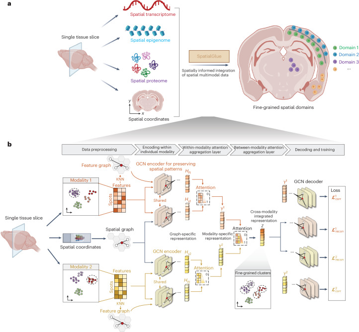
Fig. 1 Interpretable deep dual-attention model for spatial multi-omics data analysis. a, SpatialGlue overview. SpatialGlue is designed to integrate the different omics modalities with spatial information to obtain a comprehensive molecular view of the tissue under study. b, SpatialGlue model structure. SpatialGlue first uses the k-nearest-neighbor (KNN) algorithm to construct a spatial neighbor graph using the spatial coordinates and a feature neighbor graph with the normalized expression data for each omics modality. Then for each modality, a GNN encoder takes in the normalized expressions and the neighbor graph to learn two graph-specific representations by iteratively aggregating representations of neighbors. To capture the importance of different graphs, we designed a within-modality attention aggregation layer to adaptively integrate graph-specific representations and obtain a modality-specific representation. Finally, to preserve the importance of different modalities, SpatialGlue uses a between-modality attention aggregation layer to adaptively integrate modality-specific representations and output the final integrated representation of spots.
Fig. 1 Interpretable deep dual-attention model for spatial multi-omics data analysis. a, SpatialGlue overview. SpatialGlue is designed to integrate the different omics modalities with spatial information to obtain a comprehensive molecular view of the tissue under study. b, SpatialGlue model structure. SpatialGlue first uses the k-nearest-neighbor (KNN) algorithm to construct a spatial neighbor graph using the spatial coordinates and a feature neighbor graph with the normalized expression data for each omics modality. Then for each modality, a GNN encoder takes in the normalized expressions and the neighbor graph to learn two graph-specific representations by iteratively aggregating representations of neighbors. To capture the importance of different graphs, we designed a within-modality attention aggregation layer to adaptively integrate graph-specific representations and obtain a modality-specific representation. Finally, to preserve the importance of different modalities, SpatialGlue uses a between-modality attention aggregation layer to adaptively integrate modality-specific representations and output the final integrated representation of spots.CC BY · PubMed Central
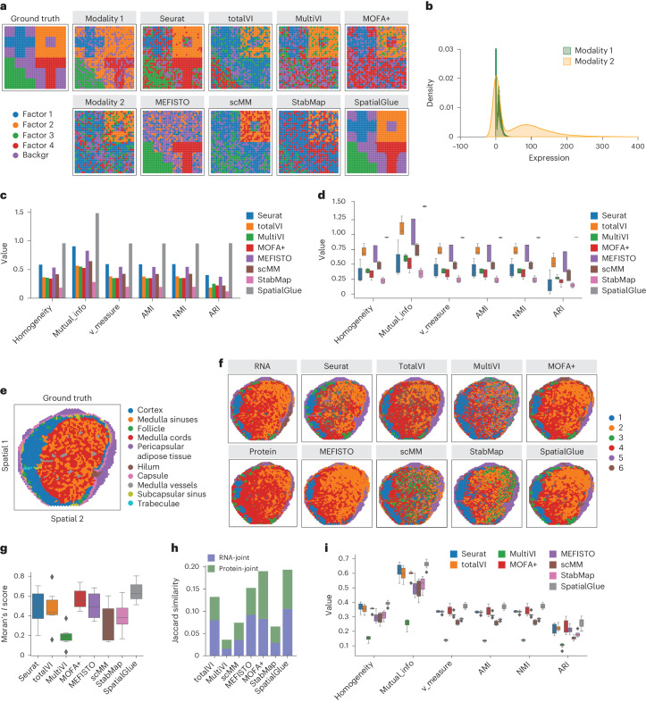
Fig. 2 SpatialGlue accurately identified spatial domains in simulated and real data. a, Spatial plots of the simulated data, from left to right: ground truth, generated raw data of individual modalities, and clustering results by single-cell and spatial multi-omics integration methods—Seurat, totalVI, MultiVI, MOFA+, MEFISTO, scMM, StabMap and SpatialGlue. ‘backgr’ means background. b, Density distribution of the simulated data modalities. c, Quantitative evaluation of methods with six supervised metrics. d, Box plots of the six metrics with the scores from five simulated datasets. In the box plot, the center line denotes the median, box limits denote the upper and lower quartiles, and whiskers denote the 1.5 times the interquartile range. n = 5 simulated samples. e, Manual annotation of human lymph node sample A1. f, Spatial plots of lymph node sample A1, clustering of individual RNA and protein modalities (left), clustering results (right) from single and spatial multi-omics integration methods—Seurat, totalVI, MultiVI, MOFA+, MEFISTO, scMM, StabMap and SpatialGlue. Note that the colors of clusters do not directly correspond to the same captured structures across different methods. g, Box plots of Moran’s I score of the eight methods. h, Jaccard similarity scores of the eight methods. In the box plot, the center line denotes the median, box limits denote the upper and lower quartiles, and whiskers denote the 1.5 times the interquartile range. n = 6 clusters. i, Box plots of six supervised metrics with scores of clustering results with the number of clusters ranging from 4 to 11. In the box plot, the center line denotes the median, box limits denote the upper and lower quartiles, and whiskers denote 1.5 times the interquartile range. n = 12 clustering results with different resolutions for each method.
Fig. 2 SpatialGlue accurately identified spatial domains in simulated and real data. a, Spatial plots of the simulated data, from left to right: ground truth, generated raw data of individual modalities, and clustering results by single-cell and spatial multi-omics integration methods—Seurat, totalVI, MultiVI, MOFA+, MEFISTO, scMM, StabMap and SpatialGlue. ‘backgr’ means background. b, Density distribution of the simulated data modalities. c, Quantitative evaluation of methods with six supervised metrics. d, Box plots of the six metrics with the scores from five simulated datasets. In the box plot, the center line denotes the median, box limits denote the upper and lower quartiles, and whiskers denote the 1.5 times the interquartile range. n = 5 simulated samples. e, Manual annotation of human lymph node sample A1. f, Spatial plots of lymph node sample A1, clustering of individual RNA and protein modalities (left), clustering results (right) from single and spatial multi-omics integration methods—Seurat, totalVI, MultiVI, MOFA+, MEFISTO, scMM, StabMap and SpatialGlue. Note that the colors of clusters do not directly correspond to the same captured structures across different methods. g, Box plots of Moran’s I score of the eight methods. h, Jaccard similarity scores of the eight methods. In the box plot, the center line denotes the median, box limits denote the upper and lower quartiles, and whiskers denote the 1.5 times the interquartile range. n = 6 clusters. i, Box plots of six supervised metrics with scores of clustering results with the number of clusters ranging from 4 to 11. In the box plot, the center line denotes the median, box limits denote the upper and lower quartiles, and whiskers denote 1.5 times the interquartile range. n = 12 clustering results with different resolutions for each method.CC BY · PubMed Central
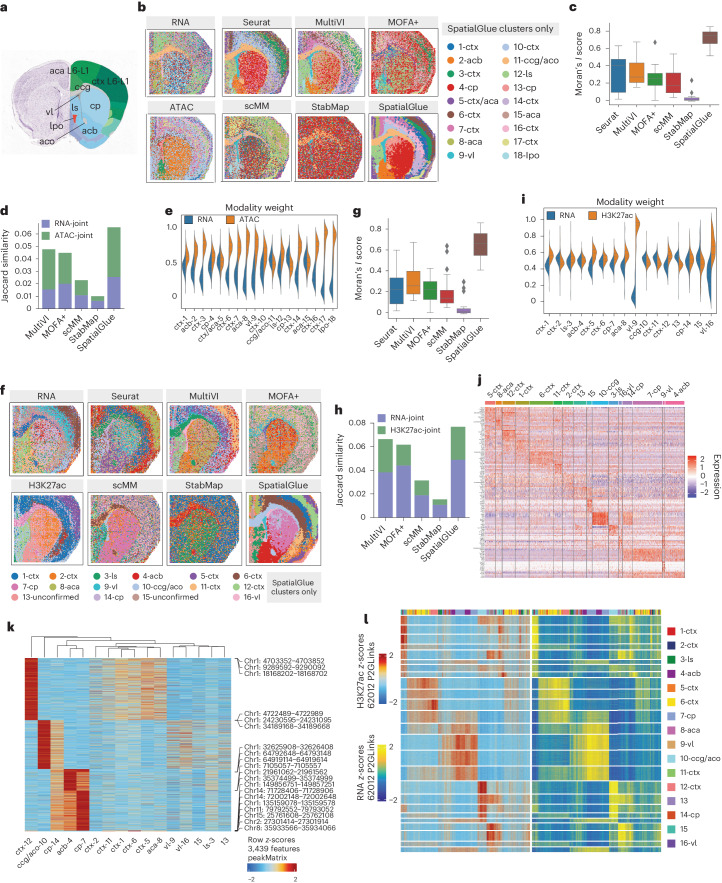
Fig. 3 SpatialGlue dissects spatial epigenome–transcriptome mouse brain samples at higher resolution. a, Annotated reference of the mouse brain coronal section from the Allen Mouse Brain Atlas. b, Spatial plots of the RNA-seq and ATAC-seq data with unimodal clustering (left) and clustering results (right) from single-cell and spatial multi-omics integration methods—Seurat, MultiVI, MOFA+, scMM, StabMap and SpatialGlue. The annotated labels correspond to SpatialGlue’s results and the clustering colors do not necessarily match to the same structures for the other methods. ctx, cerebral cortex; cp, caudoputamen; vl, lateral ventricle; lpo, lateral preoptic area; aca, anterior cingulate area; ls, lateral septal nucleus; aco, anterior commissure (olfactory limb); acb, nucleus accumbens; cc, corpus callosum. c, Box plots of Moran’s I score of the six methods. In the box plot, the center line denotes the median, box limits denote the upper and lower quartiles, and whiskers denote 1.5 times the interquartile range. n = 18 clusters. d, Comparison of Jaccard similarity scores of the six methods. e, Modality weights of different modalities, denoting their importance to the integrated output of SpatialGlue. f, Spatial plots of the RNA-seq and CUT&Tag-seq (H3K27ac) data with unimodal clustering (left), and clustering results (right) from single-cell and spatial multi-omics integration methods—Seurat, MultiVI, MOFA+, scMM, StabMap and SpatialGlue. The annotated labels correspond to SpatialGlue’s results and the clustering colors do not necessarily match to the same structures for the other methods. g, Box plots of Moran’s I score of the six methods. In the box plot, the center line denotes the median, box limits denote the upper and lower quartiles, and whiskers denote 1.5 times the interquartile range. n = 16 clusters. h, Comparison of Jaccard similarity scores of the six methods. i, Modality weights of different modalities, denoting their importance to the integrated output of SpatialGlue. j, Heat map of DEGs for each cluster. k, Heat map of differentially expressed peaks for each cluster. l, Heat map of peak-to-gene links.
Fig. 3 SpatialGlue dissects spatial epigenome–transcriptome mouse brain samples at higher resolution. a, Annotated reference of the mouse brain coronal section from the Allen Mouse Brain Atlas. b, Spatial plots of the RNA-seq and ATAC-seq data with unimodal clustering (left) and clustering results (right) from single-cell and spatial multi-omics integration methods—Seurat, MultiVI, MOFA+, scMM, StabMap and SpatialGlue. The annotated labels correspond to SpatialGlue’s results and the clustering colors do not necessarily match to the same structures for the other methods. ctx, cerebral cortex; cp, caudoputamen; vl, lateral ventricle; lpo, lateral preoptic area; aca, anterior cingulate area; ls, lateral septal nucleus; aco, anterior commissure (olfactory limb); acb, nucleus accumbens; cc, corpus callosum. c, Box plots of Moran’s I score of the six methods. In the box plot, the center line denotes the median, box limits denote the upper and lower quartiles, and whiskers denote 1.5 times the interquartile range. n = 18 clusters. d, Comparison of Jaccard similarity scores of the six methods. e, Modality weights of different modalities, denoting their importance to the integrated output of SpatialGlue. f, Spatial plots of the RNA-seq and CUT&Tag-seq (H3K27ac) data with unimodal clustering (left), and clustering results (right) from single-cell and spatial multi-omics integration methods—Seurat, MultiVI, MOFA+, scMM, StabMap and SpatialGlue. The annotated labels correspond to SpatialGlue’s results and the clustering colors do not necessarily match to the same structures for the other methods. g, Box plots of Moran’s I score of the six methods. In the box plot, the center line denotes the median, box limits denote the upper and lower quartiles, and whiskers denote 1.5 times the interquartile range. n = 16 clusters. h, Comparison of Jaccard similarity scores of the six methods. i, Modality weights of different modalities, denoting their importance to the integrated output of SpatialGlue. j, Heat map of DEGs for each cluster. k, Heat map of differentially expressed peaks for each cluster. l, Heat map of peak-to-gene links.CC BY · PubMed Central
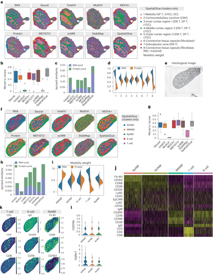
Fig. 4 SpatialGlue accurately integrates multimodal data from the mouse thymus (RNA and protein acquired with Stereo-CITE-seq) and mouse spleen (RNA and protein acquired using SPOTS). a, Spatial plots of RNA and protein data (mouse thymus acquired with Stereo-CITE-seq) with unimodal clustering (left), and comparison of clustering results (right) from single-cell and spatial multi-omics integration methods—Seurat, totalVI, MultiVI, MOFA+, MEFISTO, scMM, StabMap and SpatialGlue. The annotated labels correspond to SpatialGlue’s results and the clustering colors do not necessarily match to the same structures for the other methods. b, Box plots of Moran’s I score of the eight methods. In the box plot, the center line denotes the median, box limits denote the upper and lower quartiles, and whiskers denote 1.5 times the interquartile range. n = 8 clusters. c, Comparison of Jaccard similarity scores of the eight methods. d, Modality weights of different modalities, denoting their importance to the integrated output of SpatialGlue. e, Histology image of the mouse spleen replicate 1 sample. f, Spatial plots RNA and protein data (mouse spleen acquired using SPOTS) with unimodal clustering (left), and clustering results (right) from single-cell and spatial multi-omics integration methods—Seurat, totalVI, MultiVI, MOFA+, MEFISTO, scMM, StabMap and SpatialGlue. RpMΦ, MMMΦ and MZMΦ are red pulp macro, CD169 + MMM and CD209a+ MZM, respectively. The annotated labels correspond to SpatialGlue’s results and the clustering colors do not necessarily match to the same structures for the other methods. g, Box plots of Moran’s I score of the eight methods. In the box plot, the center line denotes the median, box limits denote the upper and lower quartiles, and whiskers denote 1.5 times the interquartile range. n = 5 clusters. h, Comparison of Jaccard similarity scores of the eight methods. i, Modality weights of different modalities, denoting their importance to the integrated output of SpatialGlue. j, Heat map of differentially expressed ADTs for each cluster. k, Normalized ADT levels of key surface markers for T cells (CD3, CD4, CD8), B cells (IgD, B220, CD19) and RpMΦ (F4_80, CD68, CD163). l, Violin plots of two marker genes in the MMMΦ, MZMΦ and RpMΦ clusters.
Fig. 4 SpatialGlue accurately integrates multimodal data from the mouse thymus (RNA and protein acquired with Stereo-CITE-seq) and mouse spleen (RNA and protein acquired using SPOTS). a, Spatial plots of RNA and protein data (mouse thymus acquired with Stereo-CITE-seq) with unimodal clustering (left), and comparison of clustering results (right) from single-cell and spatial multi-omics integration methods—Seurat, totalVI, MultiVI, MOFA+, MEFISTO, scMM, StabMap and SpatialGlue. The annotated labels correspond to SpatialGlue’s results and the clustering colors do not necessarily match to the same structures for the other methods. b, Box plots of Moran’s I score of the eight methods. In the box plot, the center line denotes the median, box limits denote the upper and lower quartiles, and whiskers denote 1.5 times the interquartile range. n = 8 clusters. c, Comparison of Jaccard similarity scores of the eight methods. d, Modality weights of different modalities, denoting their importance to the integrated output of SpatialGlue. e, Histology image of the mouse spleen replicate 1 sample. f, Spatial plots RNA and protein data (mouse spleen acquired using SPOTS) with unimodal clustering (left), and clustering results (right) from single-cell and spatial multi-omics integration methods—Seurat, totalVI, MultiVI, MOFA+, MEFISTO, scMM, StabMap and SpatialGlue. RpMΦ, MMMΦ and MZMΦ are red pulp macro, CD169 + MMM and CD209a+ MZM, respectively. The annotated labels correspond to SpatialGlue’s results and the clustering colors do not necessarily match to the same structures for the other methods. g, Box plots of Moran’s I score of the eight methods. In the box plot, the center line denotes the median, box limits denote the upper and lower quartiles, and whiskers denote 1.5 times the interquartile range. n = 5 clusters. h, Comparison of Jaccard similarity scores of the eight methods. i, Modality weights of different modalities, denoting their importance to the integrated output of SpatialGlue. j, Heat map of differentially expressed ADTs for each cluster. k, Normalized ADT levels of key surface markers for T cells (CD3, CD4, CD8), B cells (IgD, B220, CD19) and RpMΦ (F4_80, CD68, CD163). l, Violin plots of two marker genes in the MMMΦ, MZMΦ and RpMΦ clusters.CC BY · PubMed Central
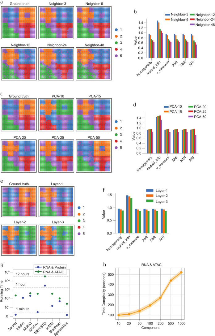
Extended Data Fig. 1 Analysis of parameter sensitivity and time complexity with simulated and real data. (a) Comparison of clustering results with different numbers of neighbors k to illustrate SpatialGlue’s sensitivity to parameters. (b) Supervised metrics on the clustering results. (c) Comparison of clustering results with different number of PCs to illustrate SpatialGlue’s sensitivity to input dimensionality. (d) Supervised metrics on the clustering results. (e) Comparison of clustering results with different numbers of GNN layers to illustrate SpatialGlue’s sensitivity to input dimensionality. (f) Supervised metrics on the clustering results. (g) Time complexity of SpatialGlue and competing methods (Seurat, totalVI, MultiVI, MOFA+, MEFISTO, scMM, StabMap). In the experiment, we used murine spleen dataset with 4,697 spots for RNA & Protein data, and mouse brain RNA ATAC P22 with 9,215 cells for RNA & ATAC data. (h) Time complexity of SpatialGlue with various principal components as inputs on mouse brain RNA ATAC P22.
Extended Data Fig. 1 Analysis of parameter sensitivity and time complexity with simulated and real data. (a) Comparison of clustering results with different numbers of neighbors k to illustrate SpatialGlue’s sensitivity to parameters. (b) Supervised metrics on the clustering results. (c) Comparison of clustering results with different number of PCs to illustrate SpatialGlue’s sensitivity to input dimensionality. (d) Supervised metrics on the clustering results. (e) Comparison of clustering results with different numbers of GNN layers to illustrate SpatialGlue’s sensitivity to input dimensionality. (f) Supervised metrics on the clustering results. (g) Time complexity of SpatialGlue and competing methods (Seurat, totalVI, MultiVI, MOFA+, MEFISTO, scMM, StabMap). In the experiment, we used murine spleen dataset with 4,697 spots for RNA & Protein data, and mouse brain RNA ATAC P22 with 9,215 cells for RNA & ATAC data. (h) Time complexity of SpatialGlue with various principal components as inputs on mouse brain RNA ATAC P22.CC BY · PubMed Central
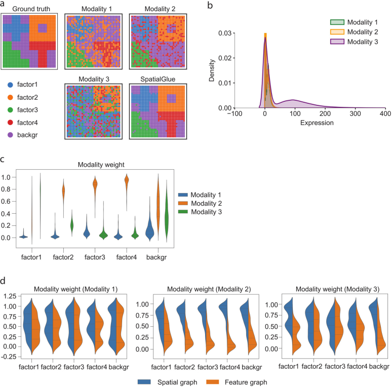
Extended Data Fig. 2 Evaluation of SpatialGlue on simulated triple omics data. (a) ground truth and spatial plots of modalities 1, 2, 3, and SpatialGlue. (b) Density distribution of simulated data modalities. (c) SpatialGlue’s between modality weights explaining the importance of each modality to each cluster. (d) Within-modality weights for the importance of spatial and feature graphs.
Extended Data Fig. 2 Evaluation of SpatialGlue on simulated triple omics data. (a) ground truth and spatial plots of modalities 1, 2, 3, and SpatialGlue. (b) Density distribution of simulated data modalities. (c) SpatialGlue’s between modality weights explaining the importance of each modality to each cluster. (d) Within-modality weights for the importance of spatial and feature graphs.CC BY · PubMed Central
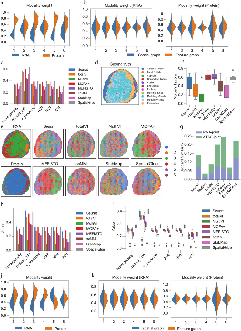
Extended Data Fig. 3 Results for lymph node samples A1 (a-c) and D1(d-k). (a) SpatialGlue’s between-modality weight explaining the importance of each modality to each cluster for the lymph node A1 sample. (b) Within-modality weights for the RNA and protein modalities explaining the contributions of the spatial and feature graphs to each cluster. (c) Quantitative evaluation of SpatialGlue and competing methods. (d) Ground truth for the lymph node D1 sample. (e) Spatial plots of RNA and protein data (left), and clustering results of single-cell and spatial multi-omics methods, Seurat, totalVI, MultiVI, MOFA+, MEFISTO, scMM, StabMap, and SpatialGlue. (f) Comparison of Moran’s I score. In the box plot, the center line denotes the median, box limits denote the upper and lower quartiles, and whiskers denote the 1.5× interquartile range. n = 6 clusters. (g) Comparison of Jaccard Similarity scores. (h) Quantitative evaluation with six supervised metrics. (i) Box plots of six supervised metrics for clustering results with number of clusters ranging from 4 to 11. In the box plot, the center line denotes the median, box limits denote the upper and lower quartiles, and whiskers denote the 1.5× interquartile range. n = 8 clustering results with different resolutions for each method. (j) Between-modality weights explaining the importance of each modality to each cluster. (k) Within-modality weights for the RNA and protein modalities explaining the contributions of the spatial and feature graphs to each cluster.
Extended Data Fig. 3 Results for lymph node samples A1 (a-c) and D1(d-k). (a) SpatialGlue’s between-modality weight explaining the importance of each modality to each cluster for the lymph node A1 sample. (b) Within-modality weights for the RNA and protein modalities explaining the contributions of the spatial and feature graphs to each cluster. (c) Quantitative evaluation of SpatialGlue and competing methods. (d) Ground truth for the lymph node D1 sample. (e) Spatial plots of RNA and protein data (left), and clustering results of single-cell and spatial multi-omics methods, Seurat, totalVI, MultiVI, MOFA+, MEFISTO, scMM, StabMap, and SpatialGlue. (f) Comparison of Moran’s I score. In the box plot, the center line denotes the median, box limits denote the upper and lower quartiles, and whiskers denote the 1.5× interquartile range. n = 6 clusters. (g) Comparison of Jaccard Similarity scores. (h) Quantitative evaluation with six supervised metrics. (i) Box plots of six supervised metrics for clustering results with number of clusters ranging from 4 to 11. In the box plot, the center line denotes the median, box limits denote the upper and lower quartiles, and whiskers denote the 1.5× interquartile range. n = 8 clustering results with different resolutions for each method. (j) Between-modality weights explaining the importance of each modality to each cluster. (k) Within-modality weights for the RNA and protein modalities explaining the contributions of the spatial and feature graphs to each cluster.CC BY · PubMed Central
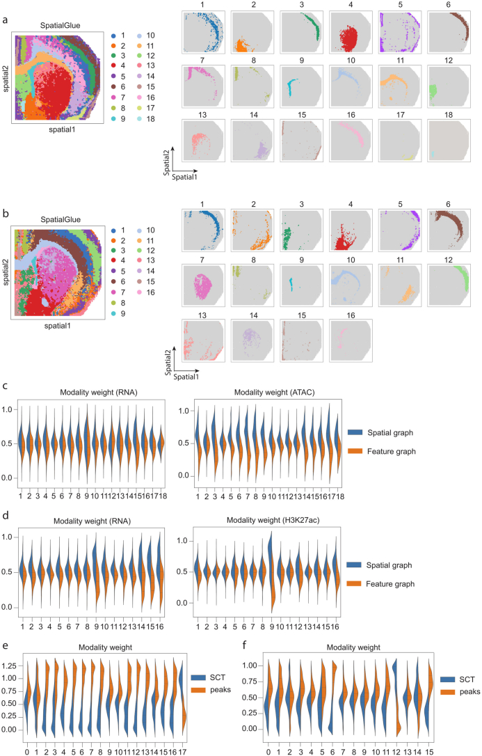
Extended Data Fig. 4 Additional results of the mouse brain P22 samples (spatial-ATAC-RNA-seq and spatial-CUT&Tag-RNA-seq, H3K27ac). (a) Separate spatial plots of all clusters identified by SpatialGlue in the mouse brain P22 sample (spatial-ATAC-RNA-seq). (b) Separate spatial plots of all clusters identified by SpatialGlue in the mouse brain P22 sample (spatial-CUT&Tag-RNA-seq, H3K27ac). (c) Within-modality weights for the RNA and ATAC modalities explaining the importance of the spatial and feature graphs to each cluster. (d) Within-modality weights for the RNA and CUT&Tag (H3K27ac) modalities explaining the importance of the spatial and feature graphs to each cluster. (e) Modality weights of Seurat when applied to the spatial-ATAC-RNA-seq P22 sample. (f) Modality weights of Seurat when applied to the spatial-CUT&Tag-RNA-seq (H3K27ac) sample.
Extended Data Fig. 4 Additional results of the mouse brain P22 samples (spatial-ATAC-RNA-seq and spatial-CUT&Tag-RNA-seq, H3K27ac). (a) Separate spatial plots of all clusters identified by SpatialGlue in the mouse brain P22 sample (spatial-ATAC-RNA-seq). (b) Separate spatial plots of all clusters identified by SpatialGlue in the mouse brain P22 sample (spatial-CUT&Tag-RNA-seq, H3K27ac). (c) Within-modality weights for the RNA and ATAC modalities explaining the importance of the spatial and feature graphs to each cluster. (d) Within-modality weights for the RNA and CUT&Tag (H3K27ac) modalities explaining the importance of the spatial and feature graphs to each cluster. (e) Modality weights of Seurat when applied to the spatial-ATAC-RNA-seq P22 sample. (f) Modality weights of Seurat when applied to the spatial-CUT&Tag-RNA-seq (H3K27ac) sample.CC BY · PubMed Central
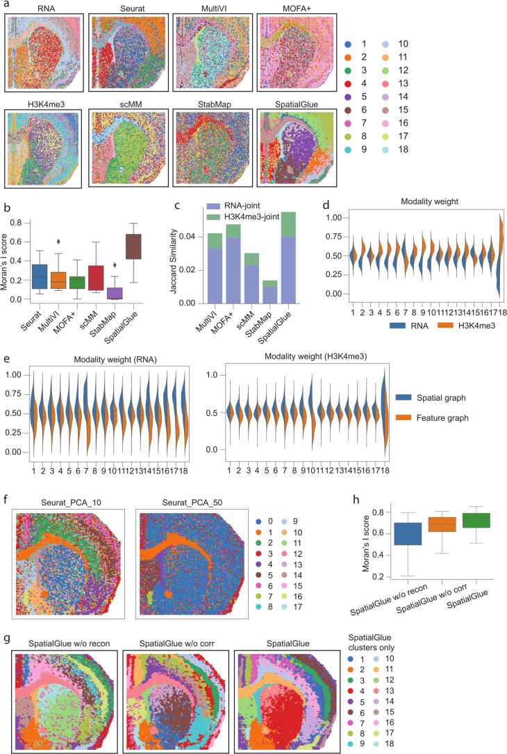
Extended Data Fig. 5 Results of the mouse brain P22 sample acquired with RNA-seq and CUT&Tag-seq (H3K4me3). (a) Spatial plots of data modalities with unimodal clustering (left), and clustering results (right) from single-cell and spatial multi-omics integration methods, Seurat, MultiVI, MOFA+, scMM, StabMap, and SpatialGlue. (b) Comparison of Moran’s I score. In the box plot, the center line denotes the median, box limits denote the upper and lower quartiles, and whiskers denote the 1.5× interquartile range. n = 18 clusters. (c) Comparison of Jaccard Similarity scores. (d) Between-modality weights explaining the importance of each modality to each cluster. (e) Within-modality weights explaining the contributions of the spatial and feature graphs to each cluster for each modality. (f) Comparison of spatial clustering using Seurat with 10 and 50 PC dimensions in the mouse brain P22 spatial-ATAC-RNA-seq sample. (g) Comparison of SpatialGlue and its variants, that is, SpatialGlue without reconstruction loss (‘SpatialGlue w/o recon’) and SpatialGlue without correspondence loss (‘SpatialGlue w/o corr’), in the mouse brain P22 spatial-ATAC-RNA-seq sample. (h) Comparison of Moran’s I score of SpatialGlue and its two variants. In the box plot, the center line denotes the median, box limits denote the upper and lower quartiles, and whiskers denote the 1.5× interquartile range. n = 18 clusters.
Extended Data Fig. 5 Results of the mouse brain P22 sample acquired with RNA-seq and CUT&Tag-seq (H3K4me3). (a) Spatial plots of data modalities with unimodal clustering (left), and clustering results (right) from single-cell and spatial multi-omics integration methods, Seurat, MultiVI, MOFA+, scMM, StabMap, and SpatialGlue. (b) Comparison of Moran’s I score. In the box plot, the center line denotes the median, box limits denote the upper and lower quartiles, and whiskers denote the 1.5× interquartile range. n = 18 clusters. (c) Comparison of Jaccard Similarity scores. (d) Between-modality weights explaining the importance of each modality to each cluster. (e) Within-modality weights explaining the contributions of the spatial and feature graphs to each cluster for each modality. (f) Comparison of spatial clustering using Seurat with 10 and 50 PC dimensions in the mouse brain P22 spatial-ATAC-RNA-seq sample. (g) Comparison of SpatialGlue and its variants, that is, SpatialGlue without reconstruction loss (‘SpatialGlue w/o recon’) and SpatialGlue without correspondence loss (‘SpatialGlue w/o corr’), in the mouse brain P22 spatial-ATAC-RNA-seq sample. (h) Comparison of Moran’s I score of SpatialGlue and its two variants. In the box plot, the center line denotes the median, box limits denote the upper and lower quartiles, and whiskers denote the 1.5× interquartile range. n = 18 clusters.CC BY · PubMed Central
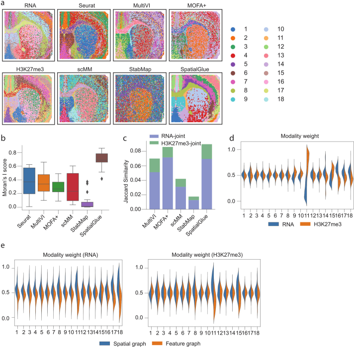
Extended Data Fig. 6 Results of the mouse brain P22 sample acquired with RNA-seq and CUT&Tag-seq (H3K27me3). (a) Spatial plots of data modalities with unimodal clustering (left), and clustering results (right) from single-cell and spatial multi-omics integration methods, Seurat, MultiVI, MOFA+, scMM, StabMap, and SpatialGlue. (b) Comparison of Moran’s I score. In the box plot, the center line denotes the median, box limits denote the upper and lower quartiles, and whiskers denote the 1.5× interquartile range. n = 18 clusters. (c) Comparison of Jaccard Similarity scores. (d) Between-modality weights explaining the importance of each modality to each cluster. (e) Within-modality weights explaining the contributions of the spatial and feature graphs to each cluster for each modality.
Extended Data Fig. 6 Results of the mouse brain P22 sample acquired with RNA-seq and CUT&Tag-seq (H3K27me3). (a) Spatial plots of data modalities with unimodal clustering (left), and clustering results (right) from single-cell and spatial multi-omics integration methods, Seurat, MultiVI, MOFA+, scMM, StabMap, and SpatialGlue. (b) Comparison of Moran’s I score. In the box plot, the center line denotes the median, box limits denote the upper and lower quartiles, and whiskers denote the 1.5× interquartile range. n = 18 clusters. (c) Comparison of Jaccard Similarity scores. (d) Between-modality weights explaining the importance of each modality to each cluster. (e) Within-modality weights explaining the contributions of the spatial and feature graphs to each cluster for each modality.CC BY · PubMed Central
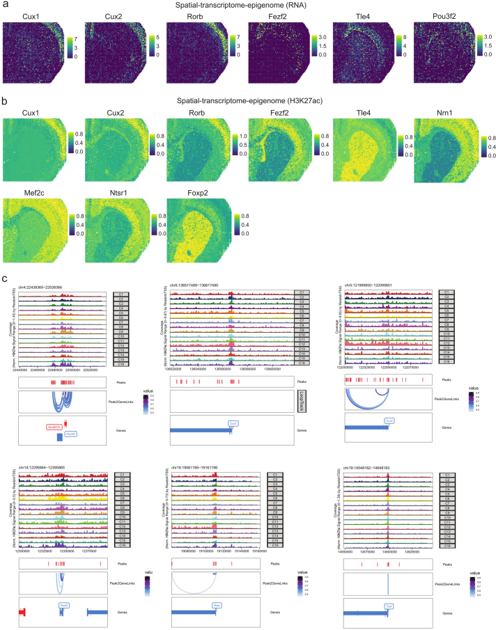
Extended Data Fig. 7 Additional results for the mouse brain P22 sample (spatial-CUT&Tag-RNA-seq, H3K27ac). (a) Intensity plots of marker genes. (b) Normalized gene activity scores from Zhang et al. (c) Peak-to-gene links plots.
Extended Data Fig. 7 Additional results for the mouse brain P22 sample (spatial-CUT&Tag-RNA-seq, H3K27ac). (a) Intensity plots of marker genes. (b) Normalized gene activity scores from Zhang et al. (c) Peak-to-gene links plots.CC BY · PubMed Central
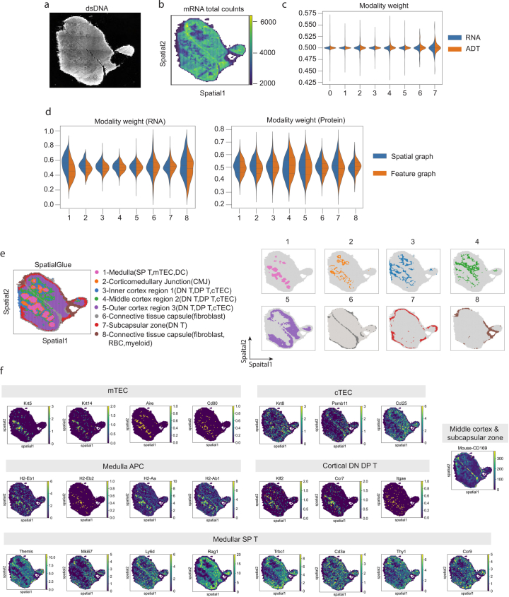
Extended Data Fig. 8 Additional results for the mouse thymus 1 sample. (a) dsDNA image. (b) Total mRNA counts. (c) Modality weight from Seurat when applied to the sample. (d) Within-modality weights of SpatialGlue explaining the contributions of the spatial and feature graphs to each cluster for each modality. (e) Separate spatial plots of all clusters identified by SpatialGlue. (f) Expression of marker genes and proteins for each cell type.
Extended Data Fig. 8 Additional results for the mouse thymus 1 sample. (a) dsDNA image. (b) Total mRNA counts. (c) Modality weight from Seurat when applied to the sample. (d) Within-modality weights of SpatialGlue explaining the contributions of the spatial and feature graphs to each cluster for each modality. (e) Separate spatial plots of all clusters identified by SpatialGlue. (f) Expression of marker genes and proteins for each cell type.CC BY · PubMed Central
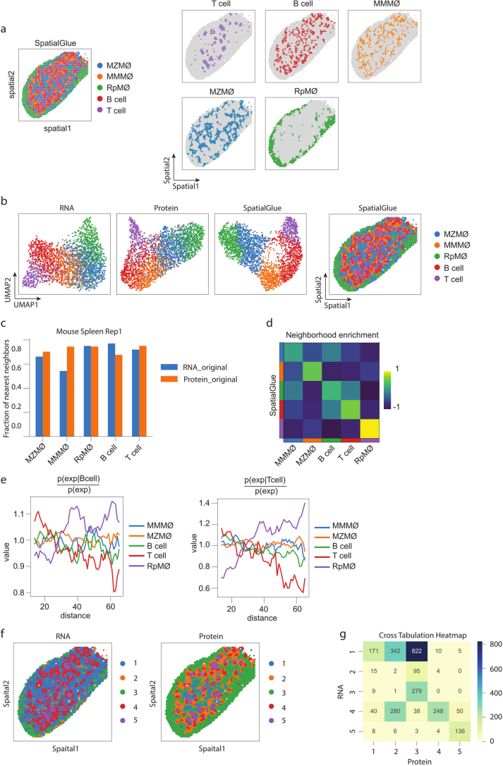
Extended Data Fig. 9 Results for the mouse spleen replicate 1 sample. (a) Spatial plots of SpatialGlue’s clusters together (left) and separate (right). (b) UMAP plots of the RNA and protein data modalities (left), and spatial plot of SpatialGlue’s clusters (right). (c) Comparison of fraction of nearest neighbors metric for each annotated cluster calculated by the different modalities (original RNA and protein expression). (d) Neighborhood enrichment of cell type pairs. (e) Cluster co-occurrence scores for each cluster at increasing distances. (f) Spatial plots of the RNA and protein data modalities. (g) Cross tabulation heatmap of the clustering labels between the RNA and protein data.
Extended Data Fig. 9 Results for the mouse spleen replicate 1 sample. (a) Spatial plots of SpatialGlue’s clusters together (left) and separate (right). (b) UMAP plots of the RNA and protein data modalities (left), and spatial plot of SpatialGlue’s clusters (right). (c) Comparison of fraction of nearest neighbors metric for each annotated cluster calculated by the different modalities (original RNA and protein expression). (d) Neighborhood enrichment of cell type pairs. (e) Cluster co-occurrence scores for each cluster at increasing distances. (f) Spatial plots of the RNA and protein data modalities. (g) Cross tabulation heatmap of the clustering labels between the RNA and protein data.CC BY · PubMed Central
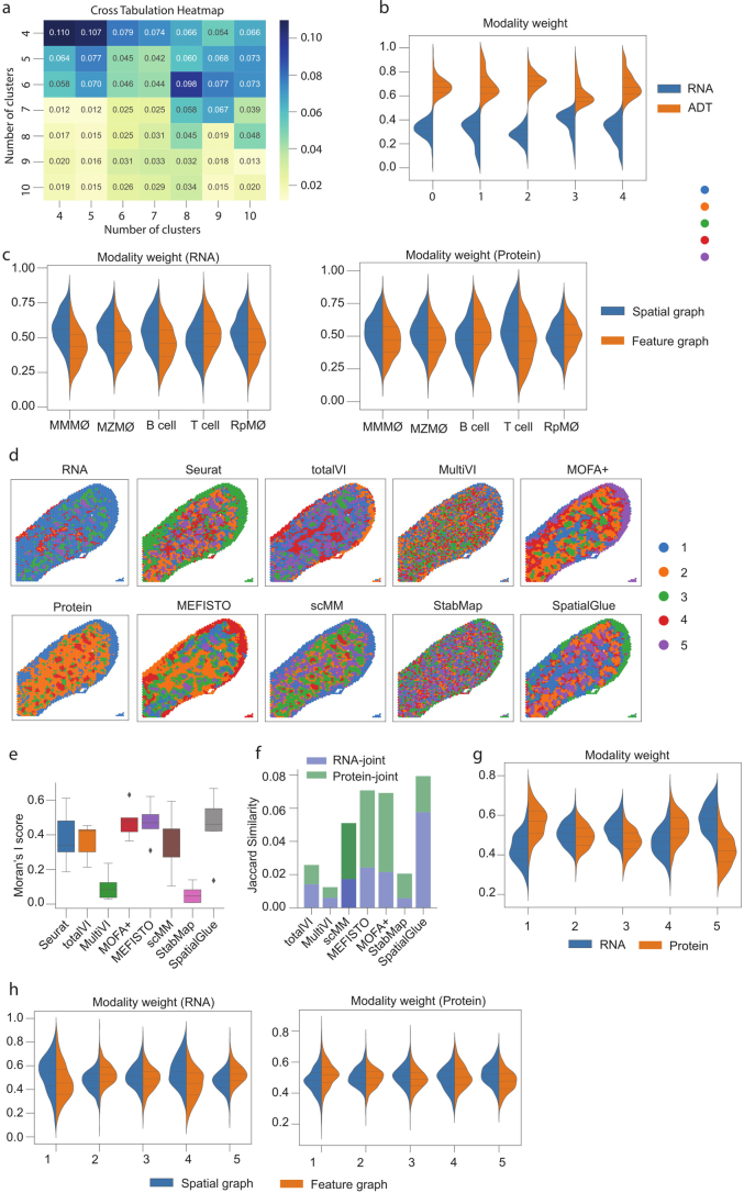
Extended Data Fig. 10 Results for the mouse spleen replicate 1(a-c) and 2(d-h) samples. (a) Cross tabulation heatmap for the number of clusters between the RNA and protein data. (b) Modality weights from Seurat. (c) Within-modality weights of SpatialGlue explaining the contributions of the spatial and feature graphs to each cluster for each modality. (d) Spatial plots of data modalities with unimodal clustering (left), and clustering results (right) from single-cell and spatial multi-omics integration methods, Seurat, totalVI, MultiVI, MOFA+, MEFISTO, scMM, StabMap, and SpatialGlue. (e) Comparison of Moran’s I score. In the box plot, the center line denotes the median, box limits denote the upper and lower quartiles, and whiskers denote the 1.5× interquartile range. n = 5 clusters. (f) Comparison of Jaccard Similarity scores. (g) Between-modality weight explaining the importance of each modality to each cluster. (h) Within-modality weights explaining the contributions of the spatial and feature graphs to each cluster for each modality.
Extended Data Fig. 10 Results for the mouse spleen replicate 1(a-c) and 2(d-h) samples. (a) Cross tabulation heatmap for the number of clusters between the RNA and protein data. (b) Modality weights from Seurat. (c) Within-modality weights of SpatialGlue explaining the contributions of the spatial and feature graphs to each cluster for each modality. (d) Spatial plots of data modalities with unimodal clustering (left), and clustering results (right) from single-cell and spatial multi-omics integration methods, Seurat, totalVI, MultiVI, MOFA+, MEFISTO, scMM, StabMap, and SpatialGlue. (e) Comparison of Moran’s I score. In the box plot, the center line denotes the median, box limits denote the upper and lower quartiles, and whiskers denote the 1.5× interquartile range. n = 5 clusters. (f) Comparison of Jaccard Similarity scores. (g) Between-modality weight explaining the importance of each modality to each cluster. (h) Within-modality weights explaining the contributions of the spatial and feature graphs to each cluster for each modality.CC BY · PubMed Central

Verification

Claims the paper makes

The claims and statistics of this paper haven’t been checked yet.

Run the check — free, no account needed. It reads the open-access text and checks the sources it cites.

A few free checks a day · papers already verified open instantly · results are public

Claims other papers make about this one

Each is checked against this paper’s own text: does it say what the citing paper says it does?

Self-check

Percentages, sums and reported differences re-computed from the paper’s own numbers.

The self-check needs the paper’s full text.

Citations

Cites

Show all 7 references

Research works printed but not linked: 20

  1. Liu, Y. et al. High-spatial-resolution multi-omics sequencing via deterministic barcoding in tissue. Cell 183, 1665–1681 (2020). · DOI · Paper page
  2. Liu, Y. et al. High-plex protein and whole transcriptome co-mapping at cellular resolution with spatial CITE-seq. Nat. Biotechnol. 41, 1405–1409 (2023). · DOI · Paper page
  3. Ben-Chetrit, N. et al. Integration of whole transcriptome spatial profiling with protein markers. Nat. Biotechnol. 41, 788–793 (2023). · DOI
  4. Vickovic, S. et al. SM-Omics is an automated platform for high-throughput spatial multi-omics. Nat. Commun. 13, 795 (2022). · DOI
  5. Liao, S. et al. Integrated spatial transcriptomic and proteomic analysis of fresh frozen tissue based on Stereo-seq. Preprint at bioRxiv https://doi.org/10.1101/2023.04.28.538364 (2023). · DOI
  6. Hudson, W. H. & Sudmeier, L. J. Localization of T cell clonotypes using the Visium spatial transcriptomics platform. STAR Protoc. 3, 101391 (2022). · DOI
  7. Janesick, A. et al. High resolution mapping of the tumor microenvironment using integrated single-cell, spatial and in situ analysis. Nat. Commun. 14, 8353 (2023). · DOI
  8. Takei, Y. et al. Integrated spatial genomics reveals global architecture of single nuclei. Nature 590, 344–350 (2021). · DOI
  9. Su, J. -H., Zheng, P., Kinrot, S. S., Bintu, B. & Zhuang, X. Genome-scale imaging of the 3D organization and transcriptional activity of chromatin. Cell 182, 1641–1659 (2020). · DOI · Paper page
  10. Liu, J. et al. Concordance of MERFISH spatial transcriptomics with bulk and single-cell RNA sequencing. Life Sci. Alliance 6, e202201701 (2023). · DOI
  11. He, S. et al. High-plex imaging of RNA and proteins at subcellular resolution in fixed tissue by spatial molecular imaging. Nat. Biotechnol. 40, 1794–1806 (2022). · DOI · Paper page
  12. Argelaguet, R. et al. MOFA+: a statistical framework for comprehensive integration of multi-modal single-cell data. Genome Biol. https://doi.org/10.1186/s13059-020-02015-1 (2020). · DOI · Paper page
  13. Ghazanfar, S., Guibentif, C. & Marioni, J. C. Stabilized mosaic single-cell data integration using unshared features. Nat. Biotechnol. 42, 284–292 (2024). · DOI
  14. Gayoso, A. et al. Joint probabilistic modeling of single-cell multi-omic data with totalVI. Nat. Methods 18, 272–282 (2021). · DOI · Paper page
  15. Minoura, K., Abe, K., Nam, H., Nishikawa, H. & Shimamura, T. A mixture-of-experts deep generative model for integrated analysis of single-cell multiomics data. Cell Rep. Methods 1, 100071 (2021). · DOI
  16. Dong, K. & Zhang, S. Deciphering spatial domains from spatially resolved transcriptomics with an adaptive graph attention auto-encoder. Nat. Commun. 13, 1739 (2022). · DOI · Paper page
  17. Alexandre, Y. O. & Mueller, S. N. Splenic stromal niches in homeostasis and immunity. Nat. Rev. Immunol. 23, 705–719 (2023). · DOI
  18. Borges da Silva, H. et al. Splenic macrophage subsets and their function during blood-borne infections. Front. Immunol. 6, 480 (2015). · DOI
  19. Backer, R. et al. Effective collaboration between marginal metallophilic macrophages and CD8+ dendritic cells in the generation of cytotoxic T cells. Proc. Natl Acad. Sci. USA 107, 216–221 (2010). · DOI
  20. Kipf, T. N. & Welling, M. Semi-supervised classification with graph convolutional networks. In 5th International Conference on Learning Representations (ICLR, 2017).

Cited by

Sorted by citations

Items 201–219 of 219

Metadata

Authors
Long, Y., Ang, K. S., Sethi, R., Liao, S., Heng, Y., van Olst, L., Ye, S., Zhong, C., Xu, H., Zhang, D., Kwok, I., Husna, N., Jian, M., Ng, L. G., Chen, A., Gascoigne, N. R. J., Gate, D., Fan, R., Xu, X., & Chen, J.
Affiliations
  • Agency for Science, Technology and Research (SG)
  • BGI Group (China) (CN)
  • Northwestern University (US)
  • Yale University (US)
  • Shanghai Jiao Tong University (CN)
  • National University of Singapore (SG)
Corresponding author
  • Chen, Ao
  • Chen, Jinmiao
Venue
Nature Methods
Published
2024-06-21
Volume
21
Issue
9
Pages
1658-1667
ISSN
  • 1548-7091 (ISSN-L)
  • 1548-7105
OpenAlex
W4399892951
Cited by
223
References
28
Citations by year
2026: 131 · 2025: 78 · 2024: 13
FWCI
30.22
Type
journal article
Language
en
Open access
Locations
  • Nature Methods (publishedVersion, cc-by)
  • Research Square (acceptedVersion, cc-by)
  • PubMed Central (publishedVersion, cc-by)
  • PubMed (publishedVersion)
Funders
  • National Research Foundation (NRF-CRP26-2021-0001)
  • National Research Foundation Singapore (NRF-CRP26-2021-0001, MOH-OFLCG18May-0003)
  • Medical Research Council
  • National Medical Research Council (MOH-OFLCG18May-0003, NMRC /OFLCG/003/2018)
  • Biomedical Research Council
Topics
  • Life Sciences › Biochemistry, Genetics and Molecular Biology › Molecular Biology › Single-cell and spatial transcriptomics
  • Life Sciences › Biochemistry, Genetics and Molecular Biology › Molecular Biology › Bioinformatics and Genomic Networks
  • Social Sciences › Economics, Econometrics and Finance › Economics and Econometrics › Spatial and Panel Data Analysis
Keywords
spatial multi-omics, spatial domain identification, graph neural networks, dual attention mechanism, transcriptome-proteome integration, spatial data integration
MeSH terms
Epigenome, Multiomics, Animals, Brain, Humans, Spleen, Neural Networks, Computer, Computational Biology, Proteome, Genomics, Proteomics, Mice, Transcriptome

About these checks

Registry, retraction, Cites and statistics results are computed, not judged, with one exception: a printed reference that no index lists is read once by a model before it counts as a citation error. Claims are extracted by a model and kept only when their quote appears verbatim in the text; each cited source is then checked, with a model’s help, for whether it says what the claim relies on. Those verdicts can be wrong — read the claim’s quote and the cited source before relying on one.

Statistics and arithmetic are recomputed, not judged.

Confidence bands are shown only for fields calibrated on our annotated test set. None is calibrated yet, so no band is shown.

What counts as a claim ›How we measure confidence ›How we check this ›

Are you an author, or do you see a problem with this page? Request a review