

The DOI matches its Crossref record; 124 of the 125 references it cites were found in a registry or an index.
A tool for mapping microglial morphology, morphOMICs, reveals brain-region and sex-dependent phenotypes
Open accessPublished version of a preprint
Abstract
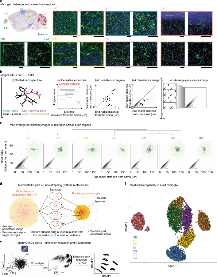
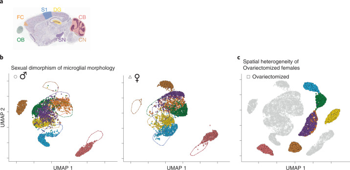
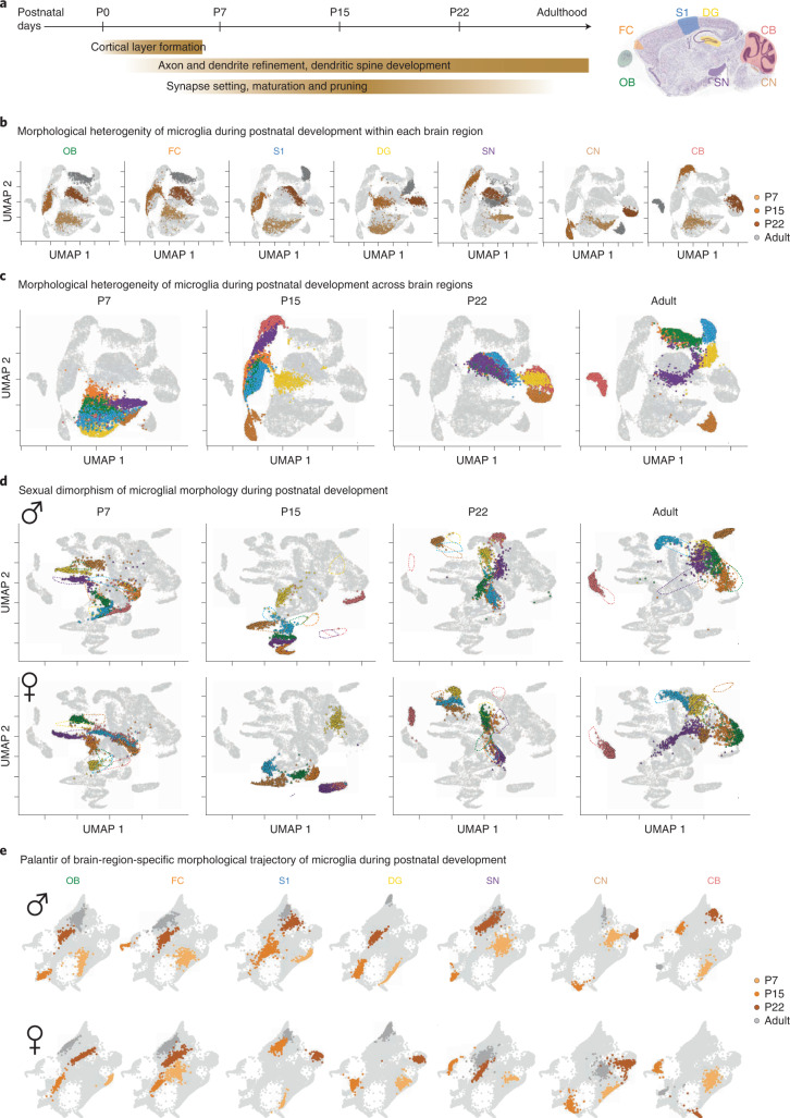
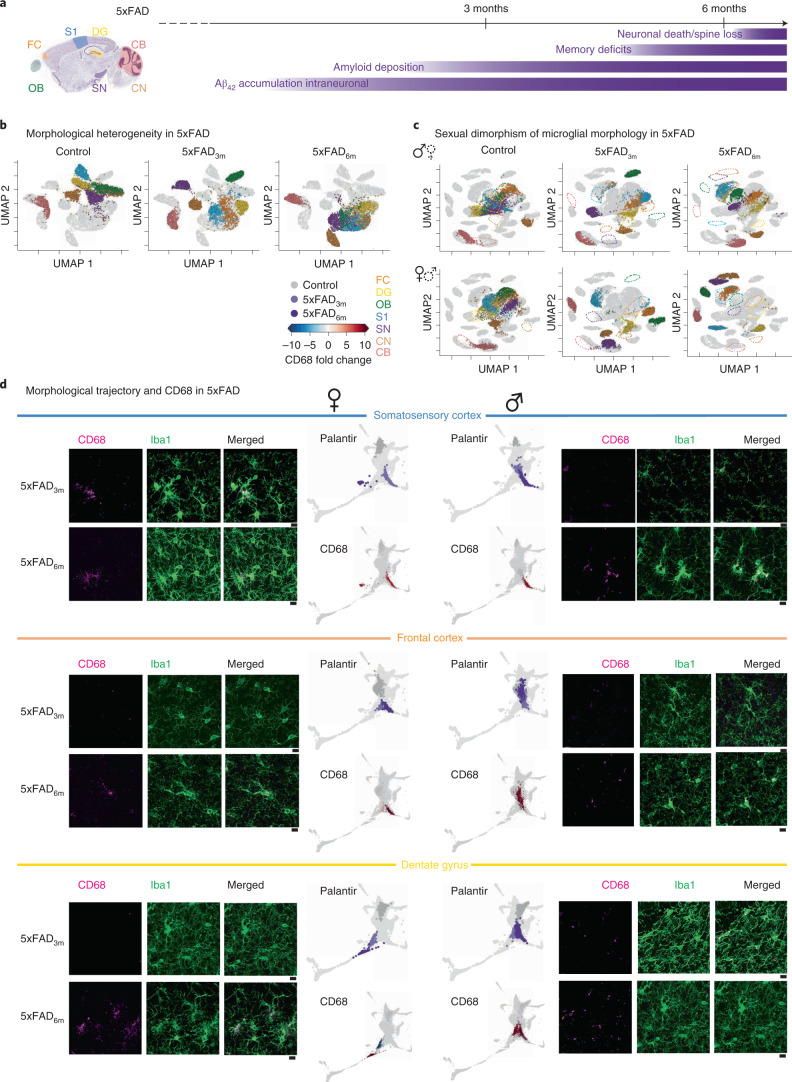
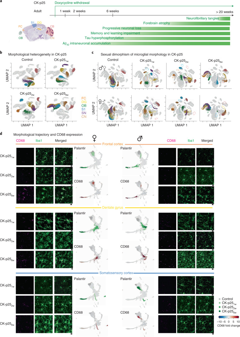
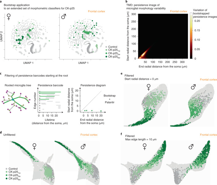
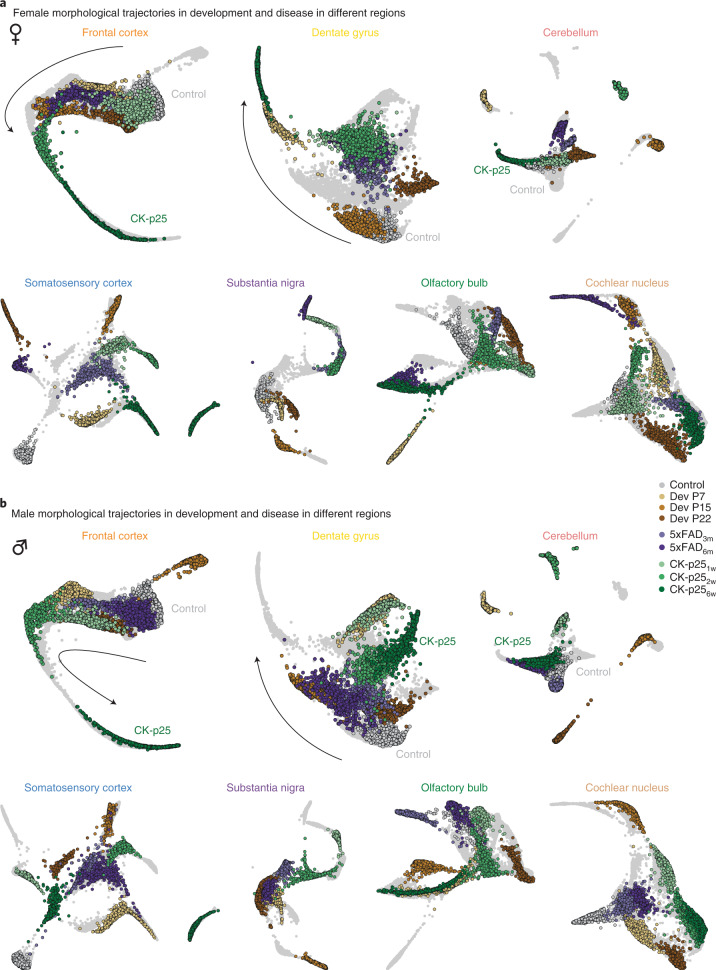
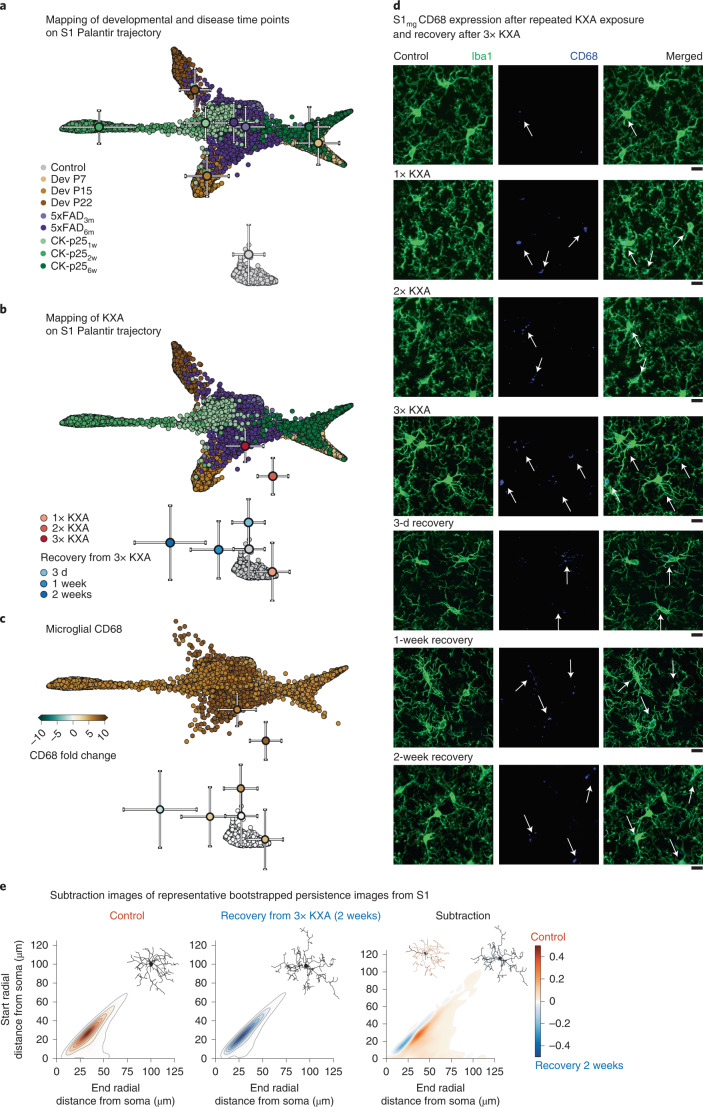
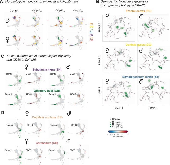
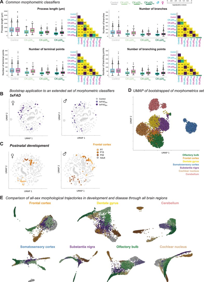
Environmental cues influence the highly dynamic morphology of microglia. Strategies to characterize these changes usually involve user-selected morphometric features, which preclude the identification of a spectrum of context-dependent morphological phenotypes. Here we develop MorphOMICs, a topological data analysis approach, which enables semiautomatic mapping of microglial morphology into an atlas of cue-dependent phenotypes and overcomes feature-selection biases and biological variability. We extract spatially heterogeneous and sexually dimorphic morphological phenotypes for seven adult mouse brain regions. This sex-specific phenotype declines with maturation but increases over the disease trajectories in two neurodegeneration mouse models, with females showing a faster morphological shift in affected brain regions. Remarkably, microglia morphologies reflect an adaptation upon repeated exposure to ketamine anesthesia and do not recover to control morphologies. Finally, we demonstrate that both long primary processes and short terminal processes provide distinct insights to morphological phenotypes. MorphOMICs opens a new perspective to characterize microglial morphology.
Overview
The claims and statistics of this paper haven’t been checked yet.
Run the check — free, no account needed. It reads the open-access text and checks the sources it cites.
Integrity signals
Registry
Cites
Statistics
Figures
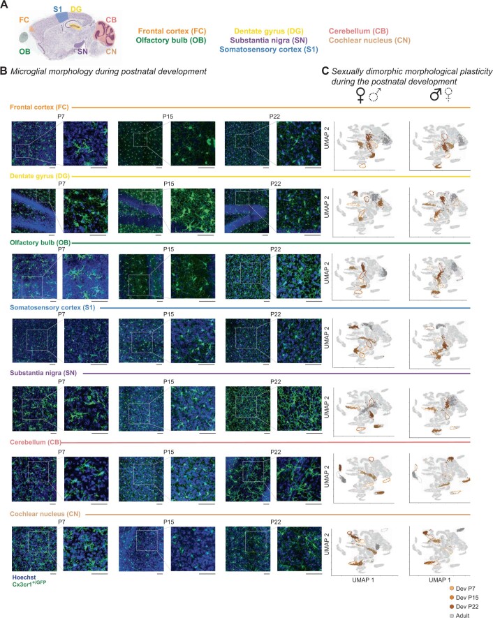
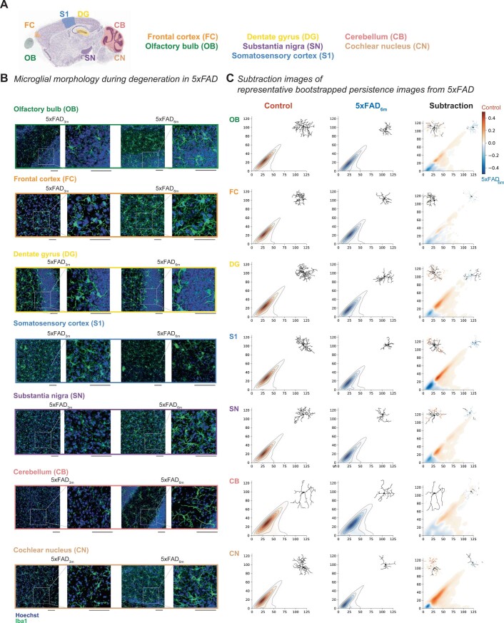
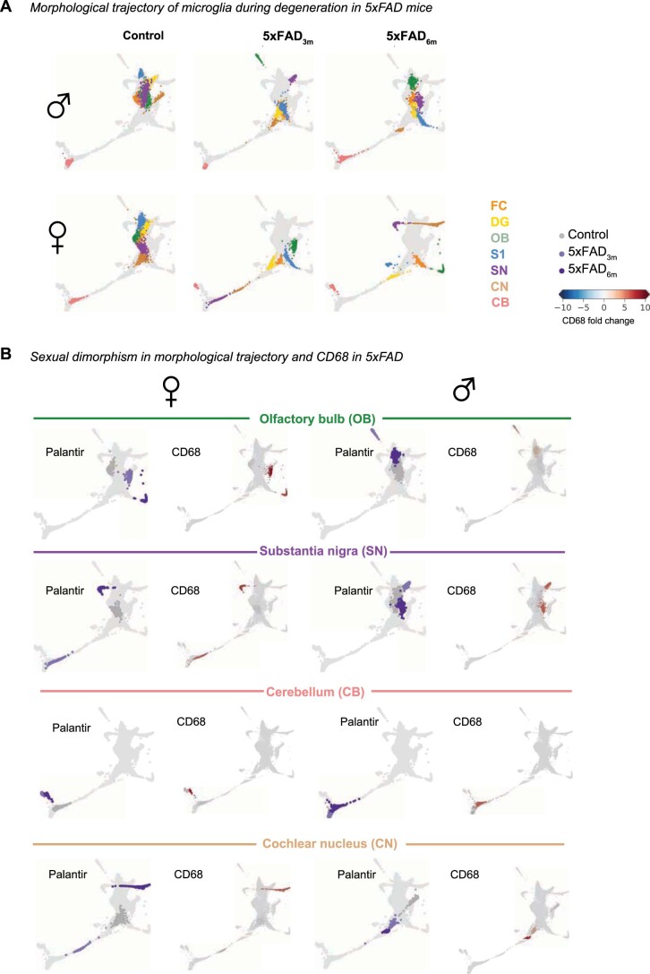
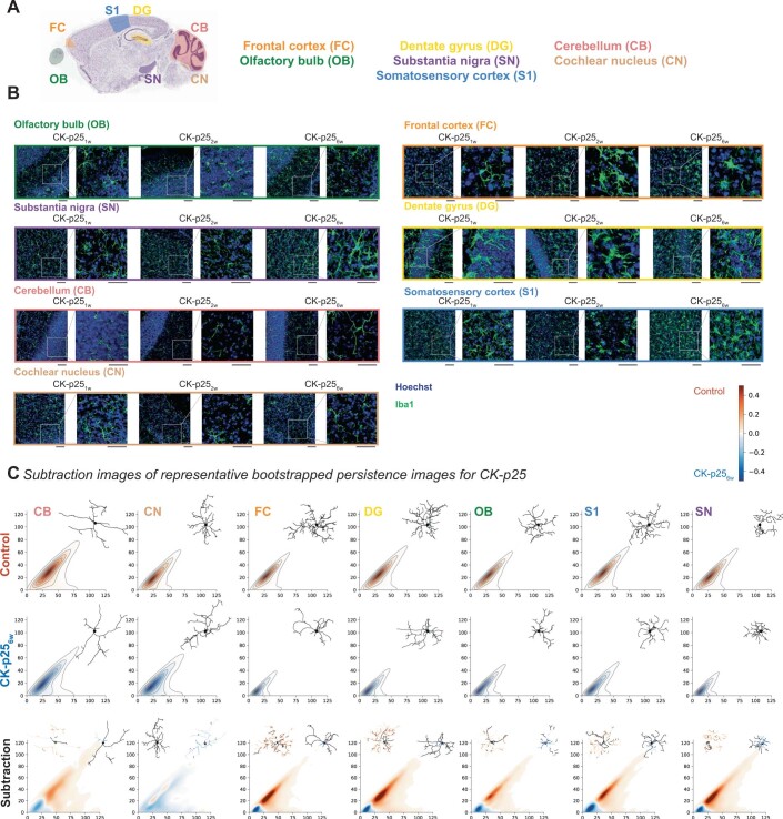
Verification
Claims the paper makes
The claims and statistics of this paper haven’t been checked yet.
Run the check — free, no account needed. It reads the open-access text and checks the sources it cites.
Claims other papers make about this one
Each is checked against this paper’s own text: does it say what the citing paper says it does?
The source backs part of the claim, not all of it — or backs it for a different population, condition or comparison.
In the citing paper
“Cells portraying smaller cellular somas in addition to extensive and well-branched processes are usually linked to a surveillant state of microglia, whereas the shrinkage of processes and bigger somas are usually linked to reactive states [83–86].”
From Sex chromosomes and sex hormones differently shape microglial properties during normal physiological conditions in the adult mouse hippocampus (2025) · cites this paper as [84]
Experimental — accuracy not yet measured
Self-check
Percentages, sums and reported differences re-computed from the paper’s own numbers.
The self-check needs the paper’s full text.
Citations
Cites
UMAP: Uniform Manifold Approximation and Projection
McInnes, L., Healy, J., Saul, N., & Großberger, L. (2018) · Journal of Open Source Software · doi:10.21105/joss.00861 · Cited by 9,826
Shrestha, S., & Offer, S. M. (2016) · Medical Epigenetics · doi:10.1159/000444713 · Cited by 8,951
Trapnell, C., Cacchiarelli, D., Grimsby, J., Pokharel, P., Li, S., Morse, M., Lennon, N. J., Livak, K. J., Mikkelsen, T. S., & Rinn, J. L. (2014) · Nature Biotechnology · doi:10.1038/nbt.2859 · Cited by 7,314
UMAP: Uniform Manifold Approximation and Projection for Dimension Reduction
McInnes, L., Healy, J., & Melville, J. (2018) · arXiv · doi:10.48550/arxiv.1802.03426 · Cited by 7,101
Resting microglial cells are highly dynamic surveillants of brain parenchyma in vivo
Nimmerjahn, A., Kirchhoff, F., & Helmchen, F. (2005) · Science · doi:10.1126/science.1110647 · Cited by 5,827
Genome-wide atlas of gene expression in the adult mouse brain
Lein, E. S., Hawrylycz, M. J., Ao, N., Ayres, M., Bensinger, A., Bernard, A., Boe, A. F., Boguski, M. S., Brockway, K. S., Byrnes, E. J., et al. (2007) · Nature · doi:10.1038/nature05453 · Cited by 5,572
Fate Mapping Analysis Reveals That Adult Microglia Derive from Primitive Macrophages
Ginhoux, F., Greter, M., Leboeuf, M., Nandi, S., See, P., Gokhan, S., Mehler, M. F., Conway, S. J., Ng, L. G., Stanley, E. R., et al. (2010) · Science · doi:10.1126/science.1194637 · Cited by 5,175
The single-cell transcriptional landscape of mammalian organogenesis
Cao, J., Spielmann, M., Qiu, X., Huang, X., Ibrahim, D. M., Hill, A. J., Zhang, F., Mundlos, S., Christiansen, L., Steemers, F. J., et al. (2019) · Nature · doi:10.1038/s41586-019-0969-x · Cited by 4,490
Synaptic Pruning by Microglia Is Necessary for Normal Brain Development
Paolicelli, R. C., Bolasco, G., Pagani, F., Maggi, L., Scianni, M., Panzanelli, P., Giustetto, M., Ferreira, T. A., Guiducci, E., Dumas, L., et al. (2011) · Science · doi:10.1126/science.1202529 · Cited by 4,244
Host microbiota constantly control maturation and function of microglia in the CNS
Erny, D., Hrabě de Angelis, A. L., Jaitin, D., Wieghofer, P., Staszewski, O., David, E., Keren-Shaul, H., Mahlakoiv, T., Jakobshagen, K., Buch, T., et al. (2015) · Nature Neuroscience · doi:10.1038/nn.4030 · Cited by 3,569
Oakley, H., Cole, S. L., Logan, S., Maus, E., Shao, P., Craft, J., Guillozet-Bongaarts, A., Ohno, M., Disterhoft, J., Van Eldik, L., et al. (2006) · The Journal of Neuroscience · doi:10.1523/jneurosci.1202-06.2006 · Cited by 3,530
Neuropathological alterations in Alzheimer disease
Serrano-Pozo, A., Frosch, M. P., Masliah, E., & Hyman, B. T. (2011) · Cold Spring Harbor Perspectives in Medicine · doi:10.1101/cshperspect.a006189 · Cited by 3,345
Excitatory actions of gaba during development: the nature of the nurture
Ben-Ari, Y. (2002) · Nature Reviews Neuroscience · doi:10.1038/nrn920 · Cited by 2,448
Limb proportions show developmental plasticity in response to embryo movement
Pollard, A. S., Charlton, B., Hutchinson, J. R., Gustafsson, T. P., McGonnell, I. M., Timmons, J. A., & Pitsillides, A. A. (2017) · Scientific Reports · doi:10.1038/srep41926 · Cited by 2,377
Synapse loss in frontal cortex biopsies in Alzheimer's disease: Correlation with cognitive severity
DeKosky, S. T., & Scheff, S. W. (1990) · Annals of Neurology · doi:10.1002/ana.410270502 · Cited by 2,376
Carlsson, G. (2009) · Bulletin of the American Mathematical Society · doi:10.1090/s0273-0979-09-01249-x · Cited by 2,302
Heterogeneity in the distribution and morphology of microglia in the normal adult mouse brain
Lawson, L. J., Perry, V. H., Dri, P., & Gordon, S. (1990) · Neuroscience · doi:10.1016/0306-4522(90)90229-w · Cited by 2,045
Feiner, N., Motone, F., Meyer, A., & Kuraku, S. (2019) · Scientific Reports · doi:10.1038/s41598-019-40055-1 · Cited by 1,988
Microglia-specific localisation of a novel calcium binding protein, Iba1
Ito, D., Imai, Y., Ohsawa, K., Nakajima, K., Fukuuchi, Y., & Kohsaka, S. (1998) · Molecular Brain Research · doi:10.1016/s0169-328x(98)00040-0 · Cited by 1,476
GARCÍA-ALONSO, C. R., Pérez, L. M., & Fernández, J. C. F. (2011) · Annals of Operations Research · doi:10.1007/s10479-011-0841-3 · Cited by 1,435
Zarow, C., Lyness, S. A., Mortimer, J. A., & Chui, H. C. (2003) · Archives of Neurology · doi:10.1001/archneur.60.3.337 · Cited by 1,003
The Role of Microglia in the Healthy Brain: Figure 1.
Tremblay, M.-È., Stevens, B., Sierra, A., Wake, H., Bessis, A., & Nimmerjahn, A. (2011) · The Journal of Neuroscience · doi:10.1523/jneurosci.4158-11.2011 · Cited by 992
MICROGLIA AS MEDIATORS OF INFLAMMATORY AND DEGENERATIVE DISEASES
González-Scarano, F., & Baltuch, G. (1999) · Annual Review of Neuroscience · doi:10.1146/annurev.neuro.22.1.219 · Cited by 984
Principles of connectivity among morphologically defined cell types in adult neocortex
Jiang, X., Shen, S., Cadwell, C. R., Berens, P., Sinz, F., Ecker, A. S., Patel, S., & Tolias, A. S. (2015) · Science · doi:10.1126/science.aac9462 · Cited by 908
Origin and differentiation of microglia
Ginhoux, F., Lim, S., Hoeffel, G., Low, D., & Huber, T. (2013) · Frontiers in Cellular Neuroscience · doi:10.3389/fncel.2013.00045 · Cited by 905
Characterization of cell fate probabilities in single-cell data with Palantir
Setty, M., Kiseliovas, V., Levine, J., Gayoso, A., Mazutis, L., & Pe’er, D. (2019) · Nature Biotechnology · doi:10.1038/s41587-019-0068-4 · Cited by 833
Microbiome Influences Prenatal and Adult Microglia in a Sex-Specific Manner
Thion, M. S., Low, D., Silvin, A., Chen, J., Grisel, P., Schulte-Schrepping, J., Blecher, R., Ulas, T., Squarzoni, P., Hoeffel, G., et al. (2018) · Cell · doi:10.1016/j.cell.2017.11.042 · Cited by 779
Assessing Reproductive Status/Stages in Mice
Caligioni, C. S. (2009) · Current Protocols in Neuroscience · doi:10.1002/0471142301.nsa04is48 · Cited by 775
CD68/macrosialin: not just a histochemical marker
Chistiakov, D. A., Killingsworth, M., Myasoedova, V. A., Orekhov, A. N., & Bobryshev, Y. V. (2016) · Laboratory Investigation · doi:10.1038/labinvest.2016.116 · Cited by 728
Young, K., & Morrison, H. W. (2018) · Journal of Visualized Experiments · doi:10.3791/57648 · Cited by 680
Sex differences in microglial colonization of the developing rat brain
Schwarz, J. M., Sholar, P. W., & Bilbo, S. D. (2012) · Journal of Neurochemistry · doi:10.1111/j.1471-4159.2011.07630.x · Cited by 672
Microglia: Dynamic Mediators of Synapse Development and Plasticity
Wu, Y., Dissing-Olesen, L., MacVicar, B. A., & Stevens, B. (2015) · Trends in Immunology · doi:10.1016/j.it.2015.08.008 · Cited by 661
Sex-specific features of microglia from adult mice
Villa, A., Gelosa, P., Castiglioni, L., Cimino, M., Rizzi, N., Pepe, G., Lolli, F., Marcello, E., Sironi, L., Vegeto, E., et al. (2018) · Cell Reports · doi:10.1016/j.celrep.2018.05.048 · Cited by 651
Mapping hippocampal and ventricular change in Alzheimer disease
Thompson, P. M., Hayashi, K. M., de Zubicaray, G. I., Janke, A. L., Rose, S., Semple, J. M., Hong, M., Herman, D. H., Gravano, D. M., Doddrell, D. M., et al. (2004) · NeuroImage · doi:10.1016/j.neuroimage.2004.03.040 · Cited by 618
Cruz, J. C., Tseng, H.-C., Goldman, J. A., Shih, H., & Tsai, L.-H. (2003) · Neuron · doi:10.1016/s0896-6273(03)00627-5 · Cited by 609
Self-citationPattern Discrimination and the Visual Cortex
Sholl, D. A., & Uttley, A. M. (1953) · Nature · doi:10.1038/171387a0 · Cited by 605
Microglial regional heterogeneity and its role in the brain
Tan, Y.-L., Yuan, Y., & Tian, L. (2020) · Molecular Psychiatry · doi:10.1038/s41380-019-0609-8 · Cited by 571
Microglial subtypes: diversity within the microglial community
Stratoulias, V., Venero, J. L., Tremblay, M., & Joseph, B. (2019) · The EMBO Journal · doi:10.15252/embj.2019101997 · Cited by 564
Microglia Are Essential to Masculinization of Brain and Behavior
Lenz, K. M., Nugent, B. M., Haliyur, R., & McCarthy, M. M. (2013) · The Journal of Neuroscience · doi:10.1523/jneurosci.1268-12.2013 · Cited by 526
Persistence Images: A Stable Vector Representation of Persistent HomologyPreprint
Adams, H., Chepushtanova, S., Emerson, T., Hanson, E., Kirby, M. J. L., Motta, F. C., Neville, R., Peterson, C., Shipman, P. D., & Ziegelmeier, L. (2015) · arXiv (Cornell University) · doi:10.48550/arxiv.1507.06217 · Cited by 517
Morrison, H. W., & Filosa, J. A. (2013) · Journal of Neuroinflammation · doi:10.1186/1742-2094-10-4 · Cited by 506
Epigenetic regulation of brain region-specific microglia clearance activity
Ayata, P., Badimon, A., Strasburger, H. J., Duff, M. K., Montgomery, S. E., Loh, Y.-H. E., Ebert, A., Pimenova, A. A., Ramirez, B. R., Chan, A. T., et al. (2018) · Nature Neuroscience · doi:10.1038/s41593-018-0192-3 · Cited by 460
Classification of electrophysiological and morphological neuron types in the mouse visual cortex
Gouwens, N. W., Sorensen, S. A., Berg, J., Lee, C., Jarsky, T., Ting, J., Sunkin, S. M., Feng, D., Anastassiou, C. A., Barkan, E., et al. (2019) · Nature Neuroscience · doi:10.1038/s41593-019-0417-0 · Cited by 456
Estrogens, Neuroinflammation, and Neurodegeneration
Villa, A., Vegeto, E., Poletti, A., & Maggi, A. (2016) · Endocrine Reviews · doi:10.1210/er.2016-1007 · Cited by 423
Fernández-Arjona, M. D. M., Grondona, J. M., Granados-Durán, P., Fernández-Llebrez, P., & López-Ávalos, M. D. (2017) · Frontiers in Cellular Neuroscience · doi:10.3389/fncel.2017.00235 · Cited by 417
The emergent landscape of the mouse gut endoderm at single-cell resolution
Nowotschin, S., Setty, M., Kuo, Y.-Y., Liu, V., Garg, V., Sharma, R., Simon, C. S., Saiz, N., Gardner, R., Boutet, S. C., et al. (2019) · Nature · doi:10.1038/s41586-019-1127-1 · Cited by 383
Antiinflammatory Effects of Estrogen on Microglial Activation
Bruce‐Keller, A. J., Keeling, J. L., Keller, J. N., Huang, F. F., Camondola, S., & Mattson, M. P. (2000) · Endocrinology · doi:10.1210/endo.141.10.7693 · Cited by 374
Hippocampal volume as an index of Alzheimer neuropathology
Gosche, K. M., Mortimer, J. A., Smith, C. D., Markesbery, W. R., & Snowdon, D. A. (2002) · Neurology · doi:10.1212/wnl.58.10.1476 · Cited by 366
Scorcioni, R., Polavaram, S., & Ascoli, G. A. (2008) · Nature Protocols · doi:10.1038/nprot.2008.51 · Cited by 354
Mildner, A., Schlevogt, B., Kierdorf, K., Böttcher, C., Erny, D., Kummer, M. P., Quinn, M., Brück, W., Bechmann, I., Heneka, M. T., et al. (2011) · The Journal of Neuroscience · doi:10.1523/jneurosci.6209-10.2011 · Cited by 351
The cerebellum in Alzheimer’s disease: evaluating its role in cognitive decline
Jacobs, H. I. L., Hopkins, D. A., Mayrhofer, H. C., Bruner, E., van Leeuwen, F. W., Raaijmakers, W., & Schmahmann, J. D. (2017) · Brain · doi:10.1093/brain/awx194 · Cited by 349
A Starring Role for Microglia in Brain Sex Differences
Lenz, K. M., & McCarthy, M. M. (2015) · The Neuroscientist · doi:10.1177/1073858414536468 · Cited by 342
Epigenetic modifications in frontal cortex from Alzheimer's disease and bipolar disorder patients
Rao, J. S., Keleshian, V. L., Klein, S. L., & Рапопорт, С. И. (2012) · Translational Psychiatry · doi:10.1038/tp.2012.55 · Cited by 305
Microglia in Alzheimer Disease: Well-Known Targets and New Opportunities
Hemonnot, A.-L., Hua, J., Ulmann, L., & Hirbec, H. (2019) · Frontiers in Aging Neuroscience · doi:10.3389/fnagi.2019.00233 · Cited by 298
Singh, N., Hopkins, S. J., Hulme, S., Galea, J. P., Hoadley, M. E., Vail, A., Hutchinson, P. J., Grainger, S., Rothwell, N. J., King, A. T., et al. (2014) · Journal of Neuroinflammation · doi:10.1186/1742-2094-11-1 · Cited by 284
Estrogen accelerates the resolution of inflammation in macrophagic cells
Villa, A. M., Rizzi, N., Vegeto, E., Ciana, P., & Maggi, A. C. (2015) · Scientific Reports · doi:10.1038/srep15224 · Cited by 283
Fischer, A., Sananbenesi, F., Pang, P. T., Lu, B., & Tsai, L.-H. (2005) · Neuron · doi:10.1016/j.neuron.2005.10.033 · Cited by 277
Self-citationBachstetter, A. D., Van Eldik, L. J., Schmitt, F. A., Neltner, J. H., Ighodaro, E. T., Webster, S. J., Patel, E., Abner, E. L., Kryscio, R. J., & Nelson, P. T. (2015) · Acta Neuropathologica Communications · doi:10.1186/s40478-015-0209-z · Cited by 258
Bakkour, A., Morris, J. C., Wolk, D. A., & Dickerson, B. C. (2013) · NeuroImage · doi:10.1016/j.neuroimage.2013.02.059 · Cited by 251
Payami, H., Zareparsi, S., Montee, K. R., Sexton, G. J., Kaye, J. A., Bird, T. D., Yu, C. E., Wijsman, E. M., Heston, L. L., Litt, M. J., et al. (1996) · PubMed Central · Cited by 248
Automated Morphological Analysis of Microglia After Stroke
Heindl, S., Gesierich, B. G., Benakis, C., Llovera, G., Duering, M., & Liesz, A. (2018) · Frontiers in Cellular Neuroscience · doi:10.3389/fncel.2018.00106 · Cited by 237
Uncovering sex differences of rodent microglia
Han, J., Fan, Y., Zhou, K., Blomgren, K., & Harris, R. A. (2021) · Journal of Neuroinflammation · doi:10.1186/s12974-021-02124-z · Cited by 224
Kozlowski, C., & Weimer, R. M. (2012) · PLoS ONE · doi:10.1371/journal.pone.0031814 · Cited by 218
Distribution of CaMKIIα expression in the brain in vivo, studied by CaMKIIα-GFP mice
Wang, X., Zhang, C., Szabó, G., & Sun, Q. (2013) · Brain Research · doi:10.1016/j.brainres.2013.04.042 · Cited by 206
Cell Death or Synaptic Loss in Alzheimer Disease
Terry, R. D. (2000) · Journal of Neuropathology & Experimental Neurology · doi:10.1093/jnen/59.12.1118 · Cited by 200
p25/Cyclin-Dependent Kinase 5 Induces Production and Intraneuronal Accumulation of Amyloid βIn Vivo
Cruz, J. C., Kim, D., Moy, L. Y., Dobbin, M. M., Sun, X., Bronson, R. T., & Tsai, L. (2006) · Journal of Neuroscience · doi:10.1523/jneurosci.3133-06.2006 · Cited by 197
Self-citationOlfactory bulb changes in Alzheimer's disease
Ohm, T. G., & Braak, H. (1987) · Acta Neuropathologica · doi:10.1007/bf00688261 · Cited by 191
Sex differences in microglial phagocytosis in the neonatal hippocampus
Nelson, L. H., Warden, S., & Lenz, K. M. (2017) · Brain, Behavior, and Immunity · doi:10.1016/j.bbi.2017.03.010 · Cited by 189
Auditory system degeneration in Alzheimer's disease
Sinha, U. K., Hollen, K. M., Rodriguez, R., & Miller, C. A. (1993) · Neurology · doi:10.1212/wnl.43.4.779 · Cited by 184
A Topological Representation of Branching Neuronal Morphologies
Kanari, L., Dłotko, P., Scolamiero, M., Levi, R., Shillcock, J. C., Hess, K. P., & Markram, H. (2017) · Neuroinformatics · doi:10.1007/s12021-017-9341-1 · Cited by 179
Self-citationThe Endogenous Estrogen Status Regulates Microglia Reactivity in Animal Models of Neuroinflammation
Vegeto, E., Belcredito, S., Ghisletti, S., Meda, C., Etteri, S., & Maggi, A. C. (2006) · Endocrinology · doi:10.1210/en.2005-1330 · Cited by 178
The pathology of the substantia nigra in Alzheimer disease with extrapyramidal signs
Burns, J. M., Galvin, J. E., Roe, C. M., Morris, J. C., & McKeel, D. W. (2005) · Neurology · doi:10.1212/01.wnl.0000158423.05224.7f · Cited by 178
Ruusuvuori, E., Li, H., Huttu, K., Palva, J. M., Smirnov, S., Rivera, C., Kaila, K., & Voipio, J. (2004) · Journal of Neuroscience · doi:10.1523/jneurosci.5176-03.2004 · Cited by 176
A Jekyll and Hyde kinase: roles for Cdk5 in brain development and disease
Cruz, J. C., & Tsai, L. (2004) · Current Opinion in Neurobiology · doi:10.1016/j.conb.2004.05.002 · Cited by 173
Self-citationLehtovirta, M., Laakso, M. P., Soininen, H. S., Helisalmi, S., Mannermaa, A., Helkala, E.-L., Partanen, K. P. L., Ryynänen, M., Vainio, P. A., Hartikainen, P. H., et al. (1995) · Neuroscience · doi:10.1016/0306-4522(95)00014-a · Cited by 172
Doxycycline Suppresses Microglial Activation by Inhibiting the P38 MAPK and NF-KB Signaling Pathways
Santa-Cecília, F. V., Socias, B., Ouidja, M. O., Sepulveda-Diaz, J. E., Acuña, L., Silva, R. L., Michel, P. P., Del-Bel, E., Cunha, T. M., & Raisman-Vozari, R. (2016) · Neurotoxicity Research · doi:10.1007/s12640-015-9592-2 · Cited by 165
Zusso, M., Methot, L., Lo, R., Greenhalgh, A. D., David, S., & Stifani, S. (2012) · The Journal of Neuroscience · doi:10.1523/jneurosci.6182-11.2012 · Cited by 163
Kovács, T., Cairns, & Lantos (1999) · Neuropathology and Applied Neurobiology · doi:10.1046/j.1365-2990.1999.00208.x · Cited by 162
Early postnatal development of pyramidal neurons across layers of the mouse medial prefrontal cortex
Kroon, T., van Hugte, E., van Linge, L., Mansvelder, H. D., & Meredith, R. M. (2019) · Scientific Reports · doi:10.1038/s41598-019-41661-9 · Cited by 161
Alzheimer's disease: amyloid plaques in the cerebellum
Braak, H., Braak, E., Böhl, J., & Lang, W. (1989) · Journal of the Neurological Sciences · doi:10.1016/0022-510x(89)90197-4 · Cited by 157
Regulation of microglia development and homeostasis.
Greter, M., & Merad, M. (2013) · Glia · doi:10.1002/glia.22408 · Cited by 141
Venturino, A., Schulz, R., De Jesús-Cortés, H., Maes, M. E., Nagy, B., Reilly-Andújar, F., Colombo, G., Cubero, R. J. A., Schoot Uiterkamp, F. E., Bear, M. F., et al. (2021) · Cell Reports · doi:10.1016/j.celrep.2021.109313 · Cited by 140
Self-citationDavalos, D., Lee, J. K., Smith, W. B., Brinkman, B. C., Ellisman, M. H., Zheng, B., & Akassoglou, K. (2007) · Journal of Neuroscience Methods · doi:10.1016/j.jneumeth.2007.11.011 · Cited by 134
Yanguas‐Casás, N., Crespo‐Castrillo, A., CEBALLOS, M. L. D., Chowen, J. A., Azcoitia, Í., Arévalo, M., & García‐Segura, L. M. (2017) · Glia · doi:10.1002/glia.23263 · Cited by 126
Furube, E., Kawai, S., Inagaki, H., Takagi, S., & Miyata, S. (2018) · Scientific Reports · doi:10.1038/s41598-018-20643-3 · Cited by 126
Synaptogenesis in the corpus striatum of infant rat
Hattori, T., & McGeer, P. L. (1973) · Experimental Neurology · doi:10.1016/0014-4886(73)90008-3 · Cited by 125
The Cerebellum in Alzheimer's Disease
Larner, A. J. (1997) · Dementia and Geriatric Cognitive Disorders · doi:10.1159/000106632 · Cited by 124
The Role of CDK5/P25 Formation/Inhibition in Neurodegeneration
Camins, A., Verdaguer, E., Folch, J., Canudas, A. M., & Pallàs, M. (2006) · Drug News & Perspectives · doi:10.1358/dnp.2006.19.8.1043961 · Cited by 124
Physiological roles of microglia during development
Pont‐Lezica, L., Béchade, C., Cantaut-Belarif, Y., Pascual, O., & Bessis, A. (2011) · Journal of Neurochemistry · doi:10.1111/j.1471-4159.2011.07504.x · Cited by 121
Valeeva, G. R., Tressard, T., Mukhtarov, M. R., Baude, A., & Khazipov, R. (2016) · Journal of Neuroscience · doi:10.1523/jneurosci.3482-15.2016 · Cited by 121
Kongsui, R., Beynon, S. B., Johnson, S. J., & Walker, F. R. (2014) · Journal of Neuroinflammation · doi:10.1186/s12974-014-0182-7 · Cited by 115
Development of vestibular afferent projections into the hindbrain and their central targets.
Maklad, A., & Fritzsch, B. (2003) · Brain Research Bulletin · doi:10.1016/s0361-9230(03)00054-6 · Cited by 113
Adeluyi, A., Guerin, L. N., Fisher, M. L., Galloway, A. L., Cole, R. D., Chan, S. S. L., Wyatt, M. D., Davis, S. W., Freeman, L. R., Ortinski, P. I., et al. (2019) · Science Advances · doi:10.1126/sciadv.aax7031 · Cited by 109
Leuba, G., Savioz, A., Vernay, A., Carnal, B., Kraftsik, R., Tardif, É., Riederer, I. M., & Riederer, B. M. (2008) · Journal of Alzheimer s Disease · doi:10.3233/jad-2008-15112 · Cited by 106
Morphological and Phagocytic Profile of Microglia in the Developing Rat Cerebellum
Perez‐Pouchoulen, M., VanRyzin, J. W., & McCarthy, M. M. (2015) · eNeuro · doi:10.1523/eneuro.0036-15.2015 · Cited by 100
Increased olfactory bulb volume and olfactory function in early blind subjects
Rombaux, P., Huart, C., Volder, A. D., Cuevas, I., Renier, L. A., Duprez, T. P. J., & Grandin, C. B. G. (2010) · Neuroreport · doi:10.1097/wnr.0b013e32833fcb8a · Cited by 92
Iron Accumulation in the Substantia Nigra of Patients With Alzheimer Disease and Parkinsonism
Brar, S., Henderson, D. L., Schenck, J. F., & Zimmerman, E. A. (2009) · Archives of Neurology · doi:10.1001/archneurol.2008.586 · Cited by 86
Gamache, J., Yun, Y., & Chiba-Falek, O. (2020) · Disease Models & Mechanisms · doi:10.1242/dmm.045211 · Cited by 84
Selective Disruption of the Cerebral Neocortex in Alzheimer's Disease
Desikan, R. S., Sabuncu, M. R., Schmansky, N. J., Reuter, M., Cabral, H., Hess, C. P., Weiner, M. W., Biffi, A., Anderson, C. D., Rosand, J. M., et al. (2010) · PLoS ONE · doi:10.1371/journal.pone.0012853 · Cited by 83
Microglial Function across the Spectrum of Age and Gender
Nissen, J. C. (2017) · International Journal of Molecular Sciences · doi:10.3390/ijms18030561 · Cited by 83
Taipa, R. J. F., Ferreira, V., Brochado, P., Robinson, A., Reis, I., Marques, F., Mann, D. M. A., Pires, M. M., & Sousa, N. (2017) · Neuropathology and Applied Neurobiology · doi:10.1111/nan.12445 · Cited by 83
Jantzie, L. L., Cheung, P., & Todd, K. G. (2005) · Journal of Cerebral Blood Flow & Metabolism · doi:10.1038/sj.jcbfm.9600025 · Cited by 80
Sex Differences in Autophagy Contribute to Female Vulnerability in Alzheimer's Disease
Congdon, E. E. (2018) · Frontiers in Neuroscience · doi:10.3389/fnins.2018.00372 · Cited by 80
Somatosensory responses in normal aging, mild cognitive impairment, and Alzheimer’s disease
Stephen, J. M., Montaño, R., Donahue, C. H., Adair, J. C., Knoefel, J. E., Qualls, C., Hart, B. L., Ranken, D. M., & Aine, C. J. (2009) · Journal of Neural Transmission · doi:10.1007/s00702-009-0343-5 · Cited by 78
Salamanca, L., Mechawar, N., Murai, K. K., Balling, R., Bouvier, D. S., & Skupin, A. (2019) · Glia · doi:10.1002/glia.23623 · Cited by 76
Metrics for comparing neuronal tree shapes based on persistent homology
Li, Y., Wang, D., Ascoli, G. A., Mitra, P. P., & Wang, Y. (2017) · PLoS ONE · doi:10.1371/journal.pone.0182184 · Cited by 73
Olfactory bulb lesions in alzheimer's disease
Struble, R. G., & Clark, H. B. (1992) · Neurobiology of Aging · doi:10.1016/0197-4580(92)90074-8 · Cited by 70
Yang, J., Zhang, J., Yu, Y., Duan, S., & Li, X. (2012) · Cerebral Cortex · doi:10.1093/cercor/bhs291 · Cited by 66
Manji, Z., Rojas, A., Wang, W., Dingledine, R. J., Varvel, N. H., & Ganesh, T. (2019) · Journal of Alzheimer s Disease · doi:10.3233/jad-180678 · Cited by 65
Statistical analysis and data mining of digital reconstructions of dendritic morphologies
Polavaram, S., Gillette, T. A., Parekh, R., & Ascoli, G. A. (2014) · Frontiers in Neuroanatomy · doi:10.3389/fnana.2014.00138 · Cited by 61
Substantia Nigra Lesions in Alzheimer Disease and Normal Aging
Kazee, A. M., Cox, C. E., & Richfield, E. K. (1995) · Alzheimer Disease & Associated Disorders · doi:10.1097/00002093-199509020-00001 · Cited by 50
Stockley, E. W., Cole, H. M., Brown, A. D., & Wheal, H. V. (1993) · Journal of Neuroscience Methods · doi:10.1016/0165-0270(93)90020-r · Cited by 48
Isolation and Phenotyping of Adult Mouse Microglial Cells
Grabert, K., & McColl, B. W. (2018) · Methods in Molecular Biology · doi:10.1007/978-1-4939-7837-3_7 · Cited by 48
Auditory brainstem nuclei in Alzheimer's disease
Ohm, T. G., & Braak, H. (1989) · Neuroscience Letters · doi:10.1016/0304-3940(89)90243-7 · Cited by 44
Wiesman, A. I., Mundorf, V. M., Casagrande, C. C., Wolfson, S. L., Johnson, C. M., May, P. E., Murman, D. L., & Wilson, T. W. (2021) · EBioMedicine · doi:10.1016/j.ebiom.2021.103638 · Cited by 34
Computational synthesis of cortical dendritic morphologies
Kanari, L., Dictus, H., Chalimourda, A., Arnaudon, A., Geit, W. A. H. V., Coste, B., Shillcock, J. C., Hess, K. P., & Markram, H. (2022) · Cell Reports · doi:10.1016/j.celrep.2022.110586 · Cited by 33
Self-citationAlzheimer’s Disease in Man and Transgenic Mice
Turner, R. S. (2001) · American Journal Of Pathology · doi:10.1016/s0002-9440(10)64026-6 · Cited by 31
Postnatal development of intrinsic GABAergic rhythms in mouse hippocampus
Wong, T. L. H., Zhang, X. L., Nassiri‐Asl, M., Wu, C. P., Carlen, P. L., & Zhang, L. (2005) · Neuroscience · doi:10.1016/j.neuroscience.2005.04.019 · Cited by 28
Estrogen and P2 Purinergic Receptor Systems in Microglia: Therapeutic Targets for Neuroprotection.
Crain, J. M., & Watters, J. J. (2010) · PubMed · doi:10.2174/1877381801002010148 · Cited by 15
Quantitative neuronal morphometry by supervised and unsupervised learning
Bijari, K., Valera, G., López‐Schier, H., & Ascoli, G. A. (2021) · STAR Protocols · doi:10.1016/j.xpro.2021.100867 · Cited by 14
Venturino, A., & Siegert, S. (2021) · STAR Protocols · doi:10.1016/j.xpro.2021.101012 · Cited by 6
Self-citationSupervised Learning Using Homology Stable Rank Kernels
Agerberg, J., Ramanujam, R., Scolamiero, M., & Chachólski, W. (2021) · Frontiers in Applied Mathematics and Statistics · doi:10.3389/fams.2021.668046 · Cited by 3
Self-citationGeneralized persistence analysis based on stable rank invariantPreprint
Riihimäki, H., & Chachólski, W. (2018) · arXiv (Cornell University) · doi:10.48550/arxiv.1807.01217 · Cited by 2
Self-citation(1953) · Europe PMC (PubMed Central)
Research works printed but not linked: 1
- Van Der Maaten, L. & Hinton, G. Visualizing data using t-SNE. J. Mach. Learn. Res. 9, 2579–2605 (2008).
Cited by
Sorted by citations
Microglia states and nomenclature: A field at its crossroads
Paolicelli, R. C., Sierra, A., Stevens, B., Tremblay, M.-E., Aguzzi, A., Ajami, B., Amit, I., Audinat, E., Bechmann, I., Bennett, M., et al. (2022) · Neuron · doi:10.1016/j.neuron.2022.10.020 · Cited by 1,973
Self-citationHuman microglial state dynamics in Alzheimer’s disease progression
Sun, N., Victor, M. B., Park, Y. P., Xiong, X., Scannail, A. N., Leary, N., Prosper, S., Viswanathan, S., Luna, X., Boix, C. A., et al. (2023) · Cell · doi:10.1016/j.cell.2023.08.037 · Cited by 462
Self-citationMicroglial morphometric analysis: so many options, so little consistency
Reddaway, J., Richardson, P., Bevan, R. J., Stoneman, J., & Palombo, M. (2023) · Frontiers in Neuroinformatics · doi:10.3389/fninf.2023.1211188 · Cited by 131
Quantifying microglial morphology: an insight into function
Green, T. R. F., & Rowe, R. K. (2024) · Clinical & Experimental Immunology · doi:10.1093/cei/uxae023 · Cited by 119
Müller, L., Benedetto, S. D., & Müller, V. (2025) · Cells · doi:10.3390/cells14010054 · Cited by 102
Metadata
- Authors
- Colombo, G., Cubero, R. J. A., Kanari, L., Venturino, A., Schulz, R., Scolamiero, M., Agerberg, J., Mathys, H., Tsai, L.-H., Chachólski, W., Hess, K., & Siegert, S.
- Affiliations
- Institute of Science and Technology Austria (AT)
- École Polytechnique Fédérale de Lausanne (CH)
- KTH Royal Institute of Technology (SE)
- Broad Institute (US)
- Corresponding author
- Siegert, Sandra
- ORCID
- Venue
- Nature Neuroscience
- Published
- 2022-09-30
- Volume
- 25
- Issue
- 10
- Pages
- 1379-1393
- ISSN
- 1097-6256 (ISSN-L)
- 1546-1726
- PMC
- PMC9534764
- OpenAlex
- W4298137907
- Cited by
- 100
- References
- 125
- Citations by year
- 2026: 25 · 2025: 23 · 2024: 31 · 2023: 15 · 2022: 5
- FWCI
- 7.20
- Type
- journal article
- Language
- en
- Open access
- hybrid
- doi.org
- Locations
- Nature Neuroscience (publishedVersion, cc-by)
- bioRxiv (Cold Spring Harbor Laboratory) (acceptedVersion, cc-by-nd)
- PubMed Central (publishedVersion, cc-by)
- PubMed (publishedVersion)
- DSpace@MIT (Massachusetts Institute of Technology) (submittedVersion, cc-by-nc)
- Infoscience (Ecole Polytechnique Fédérale de Lausanne) (submittedVersion, cc-by-nc-nd)
- SDL (submittedVersion)
- Funders
- JPB Foundation
- Institute of Science and Technology Austria (715571, 754411)
- European Commission (HORIZON2020, 754411)
- École Polytechnique Fédérale de Lausanne
- Bundesministerium für Wissenschaft, Forschung und Wirtschaft
- Board of the Swiss Federal Institutes of Technology
- National Institutes of Health
- National Institute of Neurological Disorders and Stroke (R37NS051874)
- H2020 Marie Skłodowska-Curie Actions (754411, HORIZON2020, 715571)
- Topics
- Life Sciences › Neuroscience › Neurology › Neuroinflammation and Neurodegeneration Mechanisms
- Life Sciences › Biochemistry, Genetics and Molecular Biology › Biophysics › Cell Image Analysis Techniques
- Life Sciences › Biochemistry, Genetics and Molecular Biology › Molecular Biology › Single-cell and spatial transcriptomics
- Keywords
- microglial morphology, morphomics, topological data analysis, sex differences, regional brain differences, microglial phenotype, neurodegeneration, ketamine anesthesia, microglial maturation, mouse brain
- MeSH terms
- Animals, Brain, Disease Models, Animal, Female, Ketamine, Male, Phenotype, Microglia, Mice
About these checks
Registry, retraction, Cites and statistics results are computed, not judged, with one exception: a printed reference that no index lists is read once by a model before it counts as a citation error. Claims are extracted by a model and kept only when their quote appears verbatim in the text; each cited source is then checked, with a model’s help, for whether it says what the claim relies on. Those verdicts can be wrong — read the claim’s quote and the cited source before relying on one.
Statistics and arithmetic are recomputed, not judged.
Confidence bands are shown only for fields calibrated on our annotated test set. None is calibrated yet, so no band is shown.
What counts as a claim ›How we measure confidence ›How we check this ›
Are you an author, or do you see a problem with this page? Request a review
